Article

The Ground to Space CALibration Experiment (G-SCALE): Simultaneous Validation of UAV, Airborne, and Satellite Imagers for Earth Observation Using Specular Targets

1
Labsphere, Inc., North Sutton, NH 03260, USA
2
Flight Research Laboratory, National Research Council of Canada, Ottawa, ON K1A-0R6, Canada
3
Digital Imaging and Remote Sensing Laboratory, Chester F. Carlson Center for Imaging Science, Rochester Institute of Technology, Rochester, NY 14623, USA
4
Maxar Technologies, Longmont, CO 80503, USA
*
Author to whom correspondence should be addressed.
Remote Sens. 2023, 15(2), 294; https://doi.org/10.3390/rs15020294
Submission received: 15 November 2022 / Revised: 21 December 2022 / Accepted: 22 December 2022 / Published: 4 January 2023

Abstract

:
The objective of the Ground to Space CALibration Experiment (G-SCALE) is to demonstrate the use of convex mirrors as a radiometric and spatial calibration and validation technology for Earth Observation assets, operating at multiple altitudes and spatial scales. Specifically, point sources with NIST-traceable absolute radiance signal are evaluated for simultaneous vicarious calibration of multi- and hyperspectral sensors in the VNIR/SWIR range, aboard Unmanned Aerial Vehicles (UAVs), manned aircraft, and satellite platforms. We introduce the experimental process, field site, instrumentation, and preliminary results of the G-SCALE, providing context for forthcoming papers that will detail the results of intercomparison between sensor technologies and remote sensing applications utilizing the mirror-based calibration approach, which is scalable across a wide range of pixel sizes with appropriate facilities. The experiment was carried out at the Rochester Institute of Technology’s Tait Preserve in Penfield, NY, USA on 23 July 2021. The G-SCALE represents a unique, international collaboration between commercial, academic, and government entities for the purpose of evaluating a novel method to improve vicarious calibration and validation for Earth Observation.

Graphical Abstract

1. Introduction

Remote sensing is utilized by a wide range of scientific, governmental, and commercial entities for Earth Observation (EO). In the solar reflective spectral regions (∼350 to 2500 nm), applications include climate and environmental science, change detection and monitoring, precision agriculture, resource extraction, commerce tracking, and defense [1,2,3,4,5]. Typical instrumentation platforms are satellites (including the International Space Station), manned aircraft, and Unmanned Aerial Vehicles (UAVs) also known as Remotely Piloted Aerial Systems (RPAS) or drones. Each of these platforms may be fitted with multiple EO sensor payloads [6,7], with advantages and disadvantages in terms of spatial, radiometric, and temporal coverage and performance. As such, a combination of data sources may be capable of enhancing the quality and type of remote sensing products that can be produced [8,9,10,11,12,13,14,15,16,17,18,19].
Merging data from multiple sensors and sensor classes is challenging and can potentially lead to large uncertainties in the quality of the merged products [13,14,17,20,21,22]. A common approach is comparison of the system under evaluation to well-calibrated systems with publicly available data, such as the Landsat or Copernicus programs, but this relies upon infrequent and geographically restricted Simultaneous Nadir Overpass (SNO) events over established calibration sites [23]. Further, there can be a significant mismatch between the Ground Sample Distances (GSDs) of agency craft (10 −> 300 m), typical small-sat and airborne (<5 m), or UAV ( < < 1 m) platforms, calling into question the comparison approach especially for small targets and heterogeneous areas of interest. Data interoperability and harmonization from multiple instruments require, therefore, both thorough characterization of the individual sensors and suitable methods of intercalibration or calibration transfer [24,25,26,27,28,29,30].

Calibration and Validation Using Specular Targets

Traditional ground-based vicarious calibration of airborne or spaceborne assets relies on diffuse reflectance surface targets to relate sensor response, in units such as DN, directly to an absolute quantity, such as radiance (W/m 2 /nm/sr) or surface reflectance. This technique can also be applied as validation, whereby the sensor’s retrieval of a target’s radiance (or reflectance) is compared to a previous field or laboratory calibration. Targets suitable for spectroradiometric calibration and validation (cal/val) activities are typically spatially large, level, flat, and homogeneous, and are devoid of any strong directional (i.e., specular or hotspot) or spectral domain features. These can be large, uniform land areas or natural features such as Railroad Valley Playa [23,31,32,33]. For higher-resolution airborne and satellite sensors [34], permanent manmade structures (e.g., concrete and asphalt surfaces) or specialized temporary cal/val materials (e.g., tarps, Permaflect® panels) are commonly employed. Multiple reflectance levels can be utilized in order to assess a sensor’s radiometric response over its dynamic range. This approach is known as the Empirical Line Method (ELM) and is an important technique in radiometric calibration [35,36,37]. In the spatial domain, high contrast targets such as coastlines, bridges, airports, or purpose-built contrast arrays are utilized to assess the imager’s Point/Line Spread Functions (PSF/LSFs), Modulation Transfer Function (MTF), resolution, and system blur metrics [38,39,40]. While these legacy methods have proven effective, there are associated limitations. For example, dedicated radiometric field calibration campaigns, often performed in remote locations, have large demands on personnel and cost and are subject to scheduling, weather, and logistical concerns. Well characterized natural targets are relatively rare, geographically limited, and must be either instrumented and/or rely on radiometric assumptions [23,41].
The novel SPecular Array Radiometric Calibration (SPARC) method (patented by Raytheon Technologies and licensed to Labsphere, Inc.) employs convex mirrors to relay the image of the solar disk to a sensor under test. This produces targets suitable for deriving absolute calibration coefficients for EO remote sensing systems in the solar reflective spectrum [42,43]. The SPARC technique provides both spatial and radiometric characterization of the sensor [44]. The radiometry of a convex mirror allows tuning for individual sensors and simplifies the optical corrections necessary for derivation of absolute radiance or surface reflectance, in comparison to diffuse reflectance targets [44]. With simultaneous solar radiometric measurements, SPARC can then be used as a cal/val reference for either at-aperture spectral radiance [44,45] or surface reflectance [35]. The sub-pixel point source nature of the mirror lends itself to a direct estimate of the Sampled PSF, the full 2D MTF, ground resolving distances, and various post-processing artifacts. The technique is inherently scalable over a wide range of spatial sampling resolutions, from decimeter (UAV) to meters (manned aircraft) to decameters (Landsat 8/9, Sentinel 2, and PRISMA). The main constraints on suitability for a given pixel size being a uniform low reflectance background with at least four times the desired pixel size in diameter, and sufficient numbers of mirrors and control equipment to produce a suitable radiance level. While the G-SCALE was limited to higher resolution satellites (<2 m pixels), future experiments at the Tait Preserve could accommodate pixels on the order of 10 m. In fact, commercial applications of SPARC currently exist which are capable of targeting pixels between 0.5 m to 60 m [45]. Hypothetically, with proper scoping, facilities, and terrain, a dedicated site could be constructed for even larger pixel sizes on the order of hundreds of meters such as MODIS (250 m).
The Ground to Space CALibration Experiment (G-SCALE) examined the intercalibration of multi- and hyperspectral sensors on satellite, aircraft, and UAV platforms in the VISNIR-SWIR spectral region. Both diffuse reflectance and SPARC reference targets were deployed. The experiment had three primary objectives. The first goal was to perform simultaneous, effective absolute radiometric calibration (or validation) of three prominent EO platforms using both the novel SPARC method and other techniques of record. The second goal was to directly compare data retrievals using the various methods for accuracy and efficacy. The third goal of G-SCALE was to generate a large, validated data set for the development of inter-platform sensing techniques through an interchange of concepts, approaches, and expertise among the teams involved. This paper provides an overview of the experiment and collected data sets, the radiometric underpinnings of the SPARC technique, and a basis for future research utilizing data collected during the G-SCALE.

2. Materials and Methods
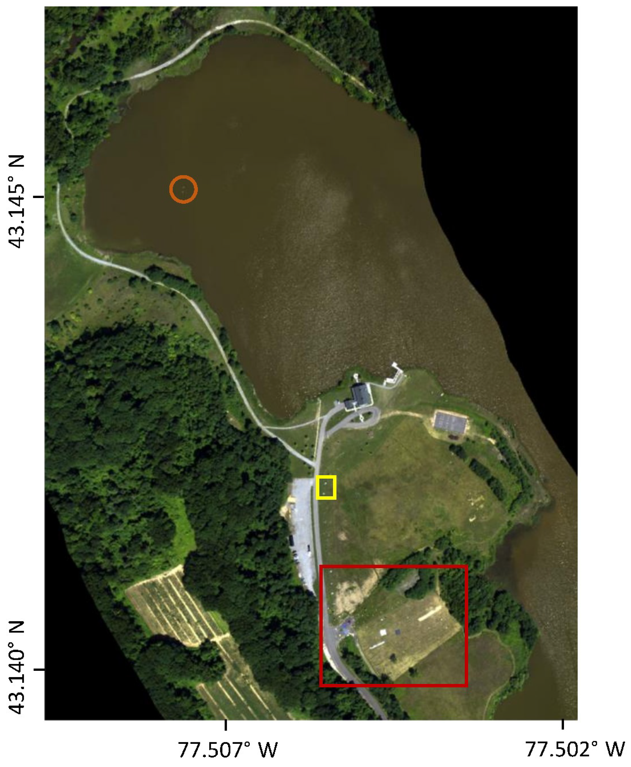
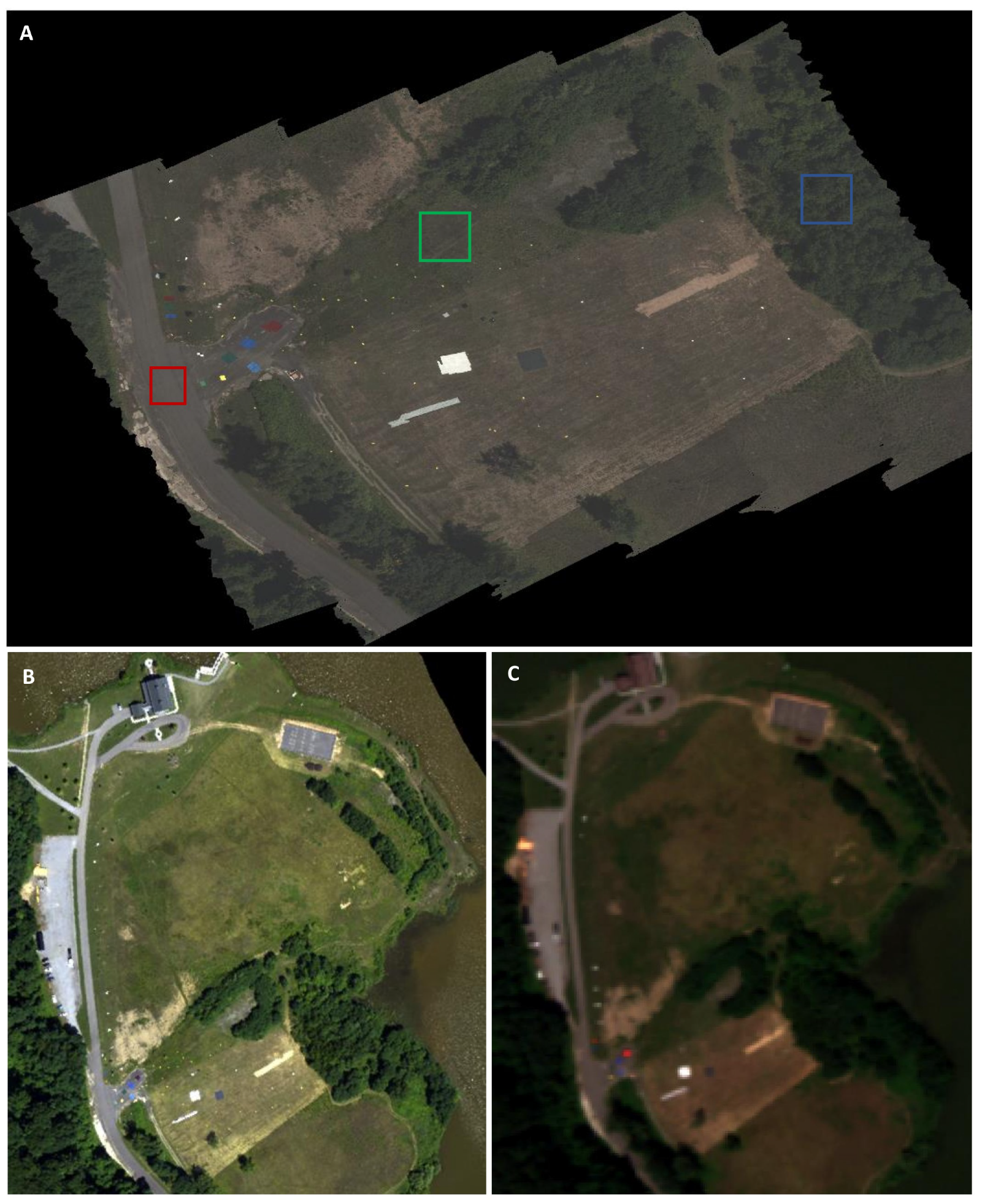
2.1. Study Area

The Ground to Space CALibration Experiment was performed at Rochester Institute of Technology’s Tait Preserve test site (Figure 1). The 177-acre property, which includes a 60-acre lake and a 5000-square-foot lodge, is located 10 miles from downtown Rochester, NY. The Tait Preserve has been used for a number of years in remote sensing data collection activities. The site has open areas of flat terrain with maintained (low-cut) grass fields, dirt and gravel plots, and asphalt and gravel roads; ideal locations for placement of targets, instrumentation, and facilities for ground data collection.

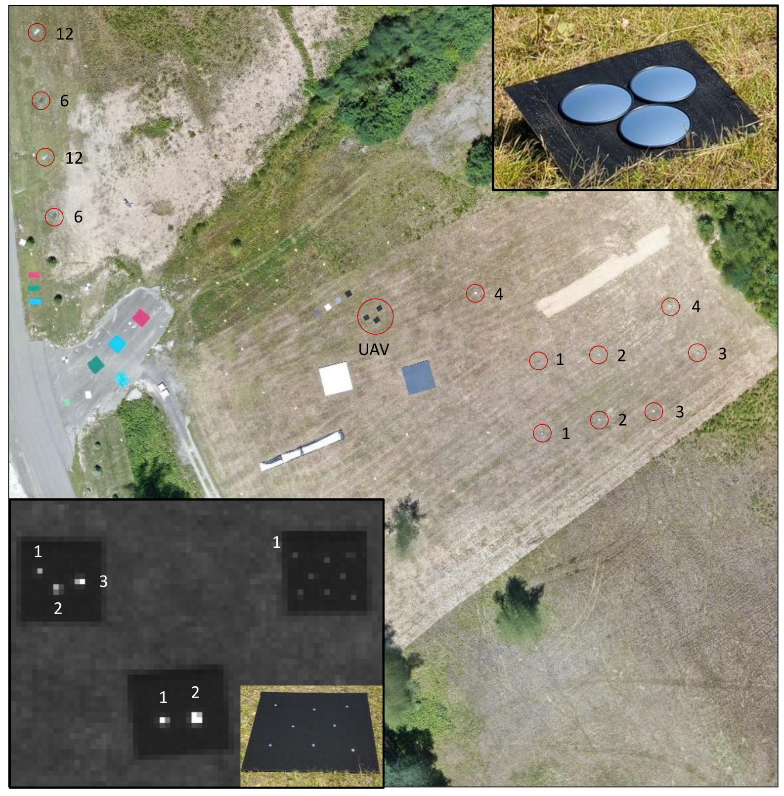
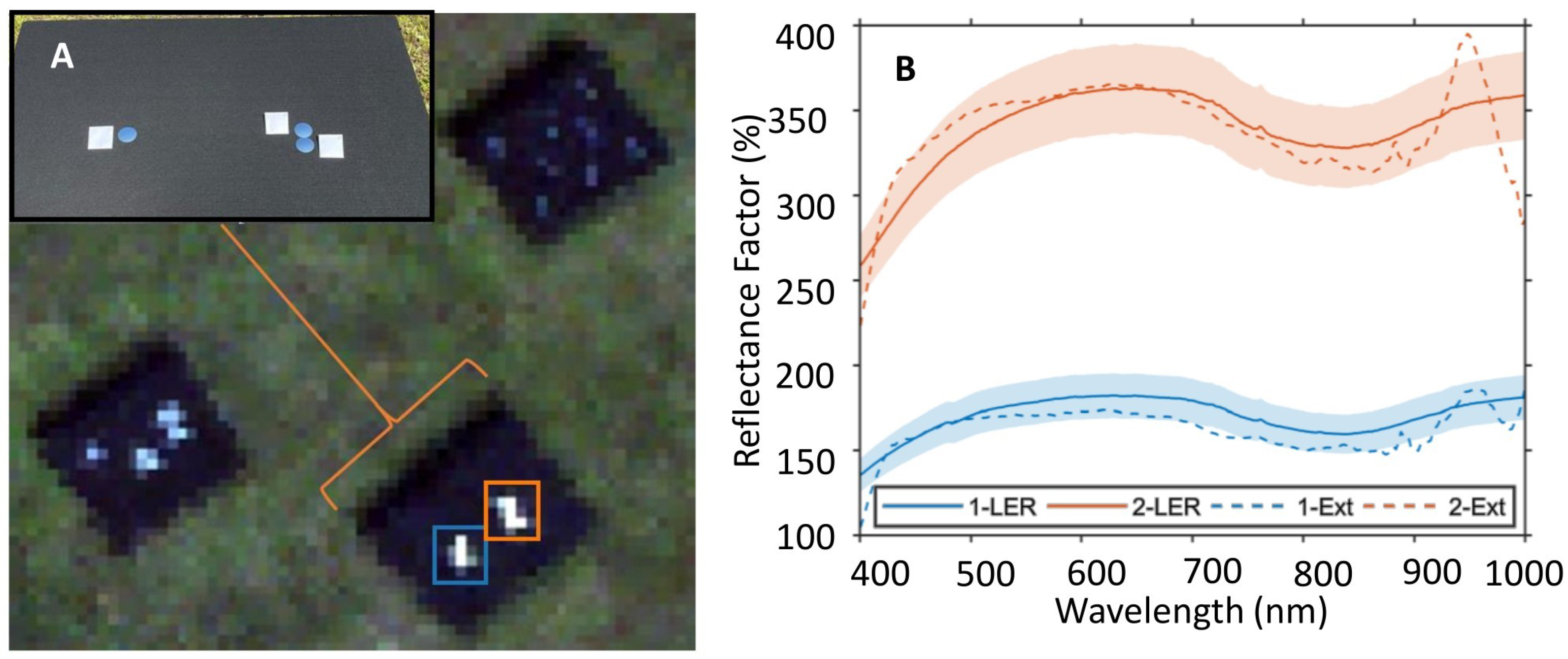
2.2. Ground Targets and Equipment

Various reference and test targets were deployed, suitable to the ground resolution of single or multiple assets. These included SPARC mirrors, diffuse spectrally flat reflectance standards, colored tarps, spectral detection targets, and spatial contrast arrays. Spectroradiometers for solar and target reflectance measurements were employed.

2.2.1. SPARC Mirrors

Multiple mirror-based targets were deployed to serve UAV, airborne, and satellite-based sensors (Figure 2). The targets were configured to provide Mirror-based Empirical Line Method (MELM) points in either reflectance or at-aperture radiance space, whereby a linear regression of instrument response against known radiance or reflectance produces a slope (calibration factor) to be applied against the imagery pixel values.
In addition to the mirrors in the primary target area and along the road, two floating mirror targets [35] were deployed on the water at the northern end of the test area (Figure 3). These targets were specifically configured for the airborne sensors to provide low-radiance calibration points optimized for dark-target, low signal-to-noise remote sensing applications such as water bodies.
It is important to note that specular target radiometry differs from traditional Lambertian radiometry [42]. The spectral at-aperture radiance L A ( λ ) and Lambertian Equivalent Reflectance Factor L E R ( λ ) of the mirrors depends on the Instantaneous Field of View (IFOV) of the sensor and slant range to the target, which is directly proportional to GSD or pixel size in resultant imagery. For example, mirror targets considered low radiance for spaceborne assets saturated the UAV-based sensors. Specific targets were configured for the GSD of the targeted sensor by varying the Radius of Curvature ( R c ), diameter, and number of mirrors. As a consequence, two distinct mirror types were utilized: one optimized for the airborne and satellite assets, and a second set of smaller mirrors deployed for use with the UAV sensors. The expected orientation of the sensor relative to the position of the mirror target on the ground and position of the sun at the time of collect must also be taken into consideration, so that the azimuth and elevation may be set to relay the solar signal. For a given sensor and mirror configuration, L A ( λ ) may be calculated:
L A ( λ ) = ρ m ( λ ) τ ( λ ) τ ( λ ) E 0 ( λ ) N R c 2 4 ( H × I F O V ) 2 D ( λ )
where:
  • ρ m : Specular reflectance of the mirrors
  • E 0 : Top of Atmosphere downwelling solar irradiance (W/m 2 /nm)
  • τ : Atmospheric transmittance from the sun to the mirror
  • τ : Atmospheric transmittance from the mirror to the sensor
  • N: Number of mirrors in a given target
  • R c : Mirror Radius of Curvature (m)
  • H: Sensor slant range aperture to mirror (m)
  • I F O V : Sensor Instantaneous Field of View (sr)
  • D: Diffuse fraction correction.
The correction for the portion of the signal contributed by reflected diffuse skylight, D ( λ ) may be calculated:
D ( λ ) = 1 + ( f G ( λ ) 1 G ( λ )
where:
  • G ( λ ) : Diffuse to global irradiance ratio measured at time of observation;
  • f = 1 cos 2 θ m : Fraction of reflected sky, with mirror Field of Regard half angle θ m .
The L A ( λ ) was computed for each SPARC target and sensor configuration. The signal can be used either to calibrate a sensor (pixel signal to radiance) or validate an existing calibration (sensor retrieved radiance vs predicted radiance).
In addition to at-aperture radiance, surface reflectance is a commonly retrieved parameter in remote sensing studies. It is possible to derive Lambertian Equivalent Reflectance (LER) [46], or the single-pixel signal equivalent to a Lambertian target of that reflectance:
L E R ( λ ) = 1 cos θ 0 + ( f 1 cos θ 0 ) G ( λ ) ρ m ( λ ) π N R c 2 4 ( H × I F O V ) 2
where:
  • θ 0 : Solar zenith angle at time of observation (°).
The L E R ( λ ) was computed for each SPARC target and sensor configuration. The signal can then serve to validate an existing surface reflectance calibration, (sensor retrieved reflectance vs predicted reflectance). For both Equations (1) and (3), the term ( H × I F O V ) 2 can be approximated by the product of the GSD in the cross and along track directions.
While Equation (1) may be employed to calibrate an entire image, in order to produce surface reflectance there is an additional step required when applying Equation (3) to a given image. When two or more SPARC targets at different radiance levels are deployed, a reflectance gain coefficient for calibrating the imagery from dimensionless number (DN) to surface reflectance ( ρ i m g ) is produced using the MELM by regression of DN to LER. As deriving this gain requires isolating the SPARC mirror target DN response from the background DN, the path radiance and background sensor bias is subtracted out and thus not known. This bias can be estimated from a measured reflectance spectrum for a dark, in-scene target and the instrument response. Finally:
ρ i m g ( λ ) = m D N ( D N i m g ( λ ) D N d r k ( λ ) ) + ρ d r k ( λ )
where:
  • m D N : Gain factor for instrument DN response to L E R , linear slope from regression of MELM targets;
  • D N i m g : Instrument response at a given image pixel;
  • ρ d r k : Measured ground-reflectance spectrum for a dark, in-scene target.
To apply the SPARC derived radiance (or reflectance) to a given image, the signal associated with the mirrors must be separated from atmospheric scattering, background, or residual sensor noise and bias [42,46]. For a given image containing SPARC points, a 7 × 7 pixel “chip” centered on each point is selected. Next, the signal within a 5 × 5 pixel radius of the center of the mirror signal is summed. This value represents both the mirror and background/atmosphere associated signals. To account for this residual, the average value of pixels in the surrounding region is subtracted from each of the pixels of interest. The final summed value (as DN, radiance, or reflectance) represents the extracted SPARC signal associated with that particular target. Note, it is assumed that the 5 × 5 region around a SPARC target will contain all of the energy associated with that target. While this assumption holds true for most well-focused sensors, the radius may be increased (or decreased) depending on the resolution of a given sensor.
While the physical size of the solar image on a mirror is dependent upon diameter and R c , this image size is negligible compared to the pixel size of the instrument under test. For example, the disk image diameter is 3 mm for the airborne and satellite mirrors and is <0.5 mm for UAV mirrors. Relative to the GSDs of each instrument, SPARC can be considered a true point source. When multiple mirrors are deployed as a single target, the physical size of the radiance source scales across all mirrors in the array. While such an extended target may not be useful for determining spatial metrics such as PSF, it is completely suitable as a radiometric source due to the signal aggregation process during image processing for the SPARC method [43].

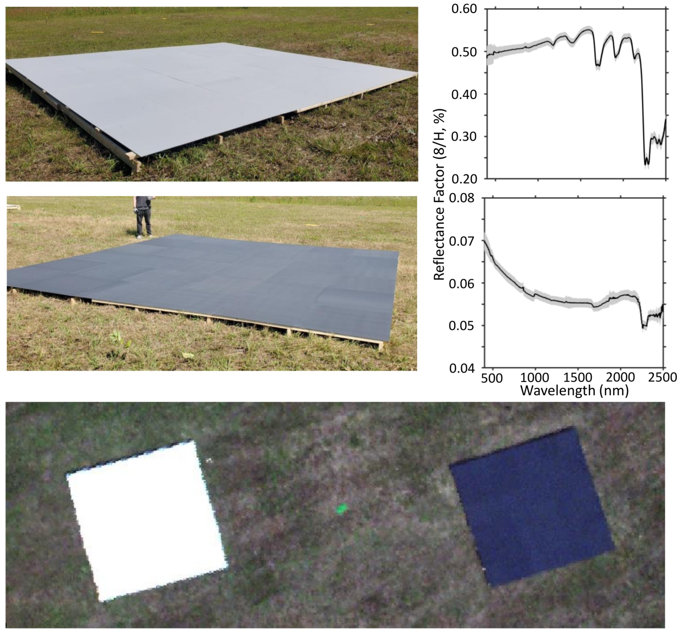
2.2.2. Permaflect® Reflectance Standards

Two large (6 m × 6 m) diffuse reflectance standards were constructed to serve as ELM reference points of approximately 5% and 50% reflectivity (Figure 4). Permaflect® (Labsphere, Inc., North Sutton, NH, USA) is a durable, weather-resistant, near-Lambertian coating that is intended for long-term use as a reflectance standard in the 250–2500 nm range. The size of the targets was selected as appropriate for UAV and airborne sensor resolutions, ensuring a large number of radiometrically accurate pixels based on the sensors’ Radiometrically Accurate Instantaneous Field-of-View (RAIFOV) [47]. The reflectance standards each consisted of 36 individual 1 m × 1 m aluminum panels, coated in either 50% or 5% (nominal reflectance) Permaflect® and laid on a raised, leveled scaffold to minimize uncertainty due to Bidirectional Reflectance Distribution Function (BRDF) or adjacency effects. It is important to note that while diffuse reflectance standards like Permaflect® and Spectralon® (Labsphere, Inc.) have a nearly Lambertian BRDF, a rigorous treatment of field reflectance measurements must include geometric correction of the standards for solar illumination and measurement angle and must take into account variations in the downwelling irradiance conditions [48]. These large, near-Lambertian targets were used to perform a reflectance-space ELM calibration of UAV and airborne imagery in order to assign surface reflectance values at each pixel. A Region of Interest (ROI) approximately 1/3 the radius of the target was extracted from each image, and the pixel values regressed against median reflectance of the panels measured during the experiment (described below).

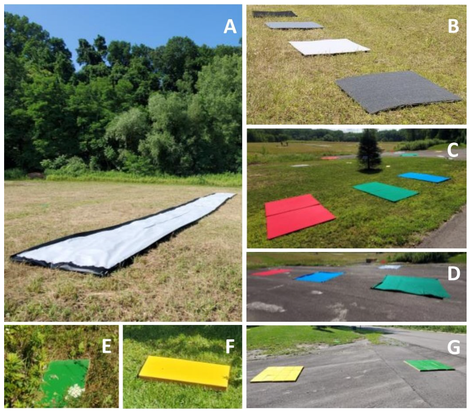
2.2.3. Diffuse Reflectance Panels and Targets

A number of diffuse reflectance targets (Figure 5) were deployed in-scene to provide calibration, validation, and test spectra. These included grey-scale tarps and panels used as calibration references for UAV platforms, colored tarps and felt panels, and numerous randomly distributed test panels for target detection and unmixing studies (Table 1). In general, the spectrally flat grey-scale targets are used for calibration of the imaging sensors by providing a known, large, level, homogeneous in-scene reference (as discussed above) that can be used to establish radiometric or reflectance gain and offset parameters. By contrast, the colored panels, tarps, and blocks deployed during the study serve as validation, or test targets, providing known signatures comparable to typical targets of interest for remote sensing applications.
The blue, green, and red colored panels (Figure 5C) have been repeatedly characterized and used in multiple large field campaigns at RIT [49,50], as well spectral image analysis studies [51,52,53,54]. The panels deployed were large fabric tarps made of 100 percent cotton dyed blue, green, and red. Two layers were placed to ensure optical thickness. These were placed over grass and pavement (Figure 5C,D). The smaller yellow and green targets (Figure 5E,F) consisted of yellow and green latex paint on a wood substrate. These wood blocks were 51 cm × 28 cm in size and scattered randomly throughout the scene on different backgrounds. Some were placed in the open while others were in brush. A total of 33 yellow and 34 green blocks were deployed. Additionally, 12 of these blocks were assembled in such a way so as to form two large yellow and green targets (Figure 5G). This large size was to ensure that there existed at least two full UAV pixels in the imagery (one yellow, one green) to use as in-scene spectral end-members useful for both spectral unmixing and spectral target detection studies.

2.2.4. Surface Measurements

An ASD FieldSpec 4 spectrometer (Malvern Panalytical) with Remote Cosine Receptor (RCR) foreoptic was deployed to measure downwelling irradiance over the course of the experiment. Measurements were made of the full sky (Figure 6B) global irradiance, with discrete shaded measurements (Figure 6C) to separate the global, direct, and diffuse components. Reflectance measurements of all the field deployed targets were made using a portable Spectra Vista Corp. (Poughkeepsie, NY, USA) (SVC) HR-1024i (336 nm to 2513 nm) with a 4°FOV fore-optic (Figure 6D) by reference to a newly produced 99% Spectralon® standard. This standard was characterized in terms of R(0°: 45°) at the National Research Council Canada (NRC) against a laboratory reference which had, in turn, been calibrated at the University of Arizona. Further adjustments for the bidirectional reflectance function of 99% Spectralon® were applied to the reference reflectance levels to adjust for the SZA at the time of the reference panel observation [48].

2.3. Remote Sensing Test Platforms

2.3.1. Unmanned Aerial Vehicles

Two primary UAVs were operated by RIT as underflight systems to the airborne and space-based platforms. The first UAV system is called the MX1-UAV. The MX1 multi-modal UAV is a modified DJI Matrice 600 and contains five sensors that collect data simultaneously. The platform contains a Headwall Nano Hyperspectral VNIR sensor (400 to 1000 nm, 270 bands), a Velodyne VLP16 LiDAR sensor, Tamarisk 640 LWIR (8–14 μ m) sensor, Mako G419 5-megapixel RBG sensor and a Micasense Red Edge Multispectral sensor. The IMU/GPS on-board the MX1 is an Applanix APX15. A second UAV, called the SWIR-UAV, was flown in tandem to the MX1. This platform contained a Headwall Hyperspectral SWIR sensor (900–2500 nm, 267 bands) and Applanix APX15 with 1–3 cm accuracy. Vehicles were flown in a raster survey of the site at an altitude of 105 m. Imagery from the two UAVs was georeferenced and processed using manufacturer provided software. A total of three surveys of the Preserve were conducted: two of the primary target area (Figure 7A) with a GSD of 6.5 cm, and a third of the northern portion of the lake over the floating SPARC targets with a GSD of 4.7 cm. Additional 75 and 100 m flights were conducted after the simultaneous overpass for additional experiments. Manufacturer provided software was used for all flight planning. A third UAV (DJI Mavic 2 Enterprise) containing a 12 megapixel CMOS camera was subsequently flown to provide at an altitude of 120 m providing hi-resolution (∼3 cm) contextual RGB imagery.
Data from the two hyperspectral sensors collected during the first survey, as well as the RGB photos, were processed to provide geo-referenced imagery that was then mosaicked over the field campaign site. The VNIR and SWIR UAV sensor platforms discussed here were not calibrated prior to the field experiment, and therefore all calibrations were performed to surface reflectance (not radiance) by ELM regression using the Permaflect® panels. The reflectance of the SPARC targets was retrieved from this imagery and compared to the expected values, as derived by Equation (3). These data were also used to compare reflectance retrievals of multiple large Regions of Interest (ROIs) for each sensor platform.

2.3.2. Airborne Hyperspectral Imagers

Two co-mounted, complimentary airborne hyperspectral systems were deployed by NRC over the Tait Preserve: the Compact Airborne Spectrographic Imager (CASI-1500, subsequently referred to as CASI) covering the spectral range from 372 nm to 1062 nm and the Shortwave Airborne Infrared Spectrographic Imager (SASI-600, subsequently referred to as SASI), covering the 957 nm to 2442 nm spectral region. Key characteristics of the two systems are provided in Table S1. The CASI and SASI sensors were deployed on a Twin Otter Turbo Prop (C-FPOK) aircraft. The sensor units are installed above a 56 cm open belly port mounted on a rigid frame loaded on the seat rails. Positional data were obtained using a Novatel OEM7 Global Positioning System (GPS) card integrated into a custom NRC data logging system with the attitudinal data supplied by a KVH-1750 Inertial Measurement Unit (IMU) mounted to the top surface of the CASI Sensor Head Unit (SHU). Geocorrection of the imagery requires precise knowledge of the lever arm lengths between the GPS antennae and IMU reference points with respect to the aperture locations of the hyperspectral imager. Positional ( δ X , δ Y , δ Z ) and attitudinal (pitch- δ ρ , roll- δ ω , heading/yaw- δ k ) lever arms, as well as the focal length and nadir pixel location within the image Field-of-View (FoV), were determined in advance using a bundling (bore-site) calibration approach [55,56,57]. Due to the relatively small variations in the study area terrain height, a fixed elevation of 793 was used in the geocorrection process rather than a Digital Elevation Model (DEM). Assessment of the geopositioning accuracy indicates that application of the 2018 derived bundling parameters were applicable to the 2021 imagery resulting in positional errors of ≤2 pixels in the along- and cross-track direction for both instruments. A total of seven overpasses were made of the target site at an altitude of 793 ± 4 m above ground (water surface) level between 15:39:21 (SZA = 31.1°) and 16:09:21 UTC (SZA = 27.3°) with a ground speed of 44 ± 2 m/s. Four of the CASI passes were performed using a sum ×3 configuration (96 channel) with an integration time (IT) of 17 ms to allow an assessment of the repeatability and spatial aliasing effect within the process under evaluation (1st, 2nd, 6th, and 7th flight lines). In addition, imagery at three additional integration times (24, 40, and 60 ms) was collected in order to assess the impact of pixel GSD on the radiometric performance of the sensors with respect to SPARC calibration targets resulting in nominal native cross-track resolutions of 0.38 m for all images with along-track resolutions of 0.75, 1.08, 1.77 and 2.68 m for the four employed ITs. SASI imagery is composed of 600 spatial pixels and 100 channels operating with a fixed frame rate (66.6 fps–16 s per frames) but with programmable IT in order to optimize the recorded signal levels. Imagery was acquired with ITs of 1.5, 2.0, 2.5, 3.0 and 3.5 ms) resulting in native cross-track resolution of 0.92 m and along-track spacing of 0.71 m.

Calibration of CASI and SASI

Nominal spectroradiometric calibration of the CASI and SASI imagery is performed using software tools and calibration files provided by the instrument manufacturer ITRES Research Ltd., Calgary, AB, Canada. The process is comprised of 5 steps: (1) identification and adjustments to account for spectral and spatial shifts in the hyperspectral systems as are typically encountered in this type of airborne system [55,58,59]; (2) offset corrections; (3) radiometric scaling; (4) smile correction; (5) geocorrection. Spectroradiometric calibration of the CASI and SASI instruments were performed by ITRES Research Ltd. using an integrating sphere on 1 November 2017 and 28 June 2018 respectively. The ITRES calibration sphere was in turn calibrated by Labsphere with respect to a NIST referenced sphere. Finally, NRC has developed and applied a refinement of the ITRES radimoetric calibration. This method uses an ELM approach making use of diffuse reflectance ground reference targets (grey and white tarps, concrete, asphalt) that have been measured using rigorous field spectroscopy techniques [48] has been incorporated into the standard processing approach performed by NRC. The imagery collected during the G-SCALE was refined with this approach, using data collected several days before the experiment. Recent experience in assessing the quality of the final radiance product for low signal level targets (i.e., water), particularly in the UV/Blue spectral range, has indicated that future refinement will require a non-linear fit be applied to such low signal data [60]. The use of low signal, SI-traceable SPARC radiance standards in vicarious calibration during flight could improve retrieval accuracy for these data.
To retrieve surface reflectance from the CASI imagery, an ELM regression was performed using the Permaflect® panels. This created a gain and offset to convert radiance values directly to in-situ surface reflectance. The reflectance of the SPARC targets was retrieved from this imagery and compared to the expected values, as derived by Equation (3). These data were also used to compare reflectance retrievals of multiple large ROIs for each sensor platform.

2.3.3. Satellites

Two EO satellites, owned and operated by Maxar, were tasked to image the Tait Preserve during the G-SCALE. GeoEye-1 launched on 6 September 2008 on a sun-synchronous orbit at an altitude of 770 km. The satellite can collect up to 500,000 km2 of imagery per day with an average revisit time of 2.3 days. The sensor geospatial accuracy is less than 5 m CE90 without ground control. A nadir view provides 0.46 and 1.84 m resolution for the panchromatic and multi-spectral bands. GeoEye-1 has four multispectral bands: blue (450–510 nm), green (510–580 nm), red (655–690 nm) and near-infrared (780–920 nm) with a dynamic range of 11 bits per pixel.
WorldView-2 launched on 8 October 2009 on a similar orbit as GeoEye-1. It has a collection capacity of 975,000 km2 per day with an average revisit time of 1.1 days. It also has geospatial accuracy of better than 5 m CE90. A nadir view provides 0.46 and 1.84 m resolution for the panchromatic and multi-spectral bands, respectively and 0.52 and 2.07 m resolution at 20° off-nadir. WorldView-2 has eight multispectral bands: coastal (400–450 nm), blue (450–510 nm), green (510–580 nm), yellow (585–625 nm), red (630–690 nm), red edge (705–745 nm), near-infrared 1 (770–895 nm) and near-infrared 2 (860–1040 nm) with a dynamic range of 11 bits per pixel.
A total of three images were collected of the Tait Preserve target area. GeoEye-1 collected two images at angles 25.9° and 31° from nadir, resulting in nominal GSDs of 0.479 m for pan and 1.920 m for the multi-band, and 0.513 m pan, 2.056 m multi-band respectively. WorldView-2 collected at angle 31.7° from nadir, resulting in nominal GSDs of 0.582 m for the pan and 2.326 m for the multi-band.

Calibration of GeoEye-1 and WorldView-2

Maxar’s primary method of radiometric calibration involves the use of the reflectance-based or vicarious calibration technique at their dedicated facility in Ft. Lupton, CO, USA. Sensor imagery is taken over 20 × 30 m specialized calibration tarps (Group 8 Technology). These diffusely reflective tarps are made to be homogeneous in both the spatial and spectral domain. Surface reflectance of the tarps is simultaneously measured at the same viewing angles as the sensor under test, while it acquires imagery of the facility. In addition, surface reflectance of the surrounding field is taken to provide information for the calculation of adjacency effects. In-situ measurements of atmospheric data such as aerosol optical depth, single scattering albedo, asymmetry parameter, column water vapor, column ozone, temperature, and pressure are also collected. These data are used in a radiative transfer model (MODTRAN 5, Spectral Sciences, Inc., Burlington, MA, USA) to provide Top of Atmosphere Radiance (ToAR), used to produce current sensor calibrations. Data are taken over 2–5 tarps regularly during the summer season from May to November to allow for a large amount of data points to be used in a regression to create the Maxar on-orbit calibration adjustments. This reflectance-based method can yield a radiometric uncertainty of ±3%, k = 1 [61]. Results are validated against secondary sites including those provided by the Radiometric Calibration Network (RadCalNet) [23]. Calibration of both satellites was carried out independently by Maxar prior to the G-SCALE, and Maxar routinely updates the coefficients of all satellite assets. The most recent updated occurred in 2018.
In addition to the ToAR product (processing Level 1B), satellite imagery was processed using Maxar’s proprietary Atmospheric Compensation (AComp) algorithm [62] to produce surface reflectance imagery. The automated AComp framework is a physics-based, first-principles atmospheric correction based on MODTRAN radiative transfer code. AComp uses an iterative process to determine and assign model parameters such as AOD using in-scene data. This surface reflectance imagery was used to compare the imagery-extracted SPARC mirror reflectance, in comparison to that predicted by Equation (3). The AComp data was also used to compare reflectance retrievals of multiple large ROIs for each sensor platform.

3. Results

The primary G-SCALE data set consists of imagery from multiple UAV mounted sensors, CASI and SASI airborne hyperspectral sensors, and GeoEye-1 and Worldview-2 satellites. Importantly, all assets imaged the site virtually simultaneously (Figure 7). In-situ solar irradiance data were continuously logged, and hyperspectral reflectance for all major targets in-scene was measured during the experiment. For the SPARC mirrors, Radius of Curvature and specular reflectance were measured previously at the Labsphere facility (North Sutton, NH, USA). The day of the experiment was extremely clear, with an occasional scattered low-altitude cloud near the horizon (Figure 6A), low winds and humidity, and a temperature between 24–27 °C. The full data set collected during G-SCALE is extremely large and will be the subject of ongoing analysis across several dimensions. A summary of the collected data, as well as example results for each platform, is presented here.

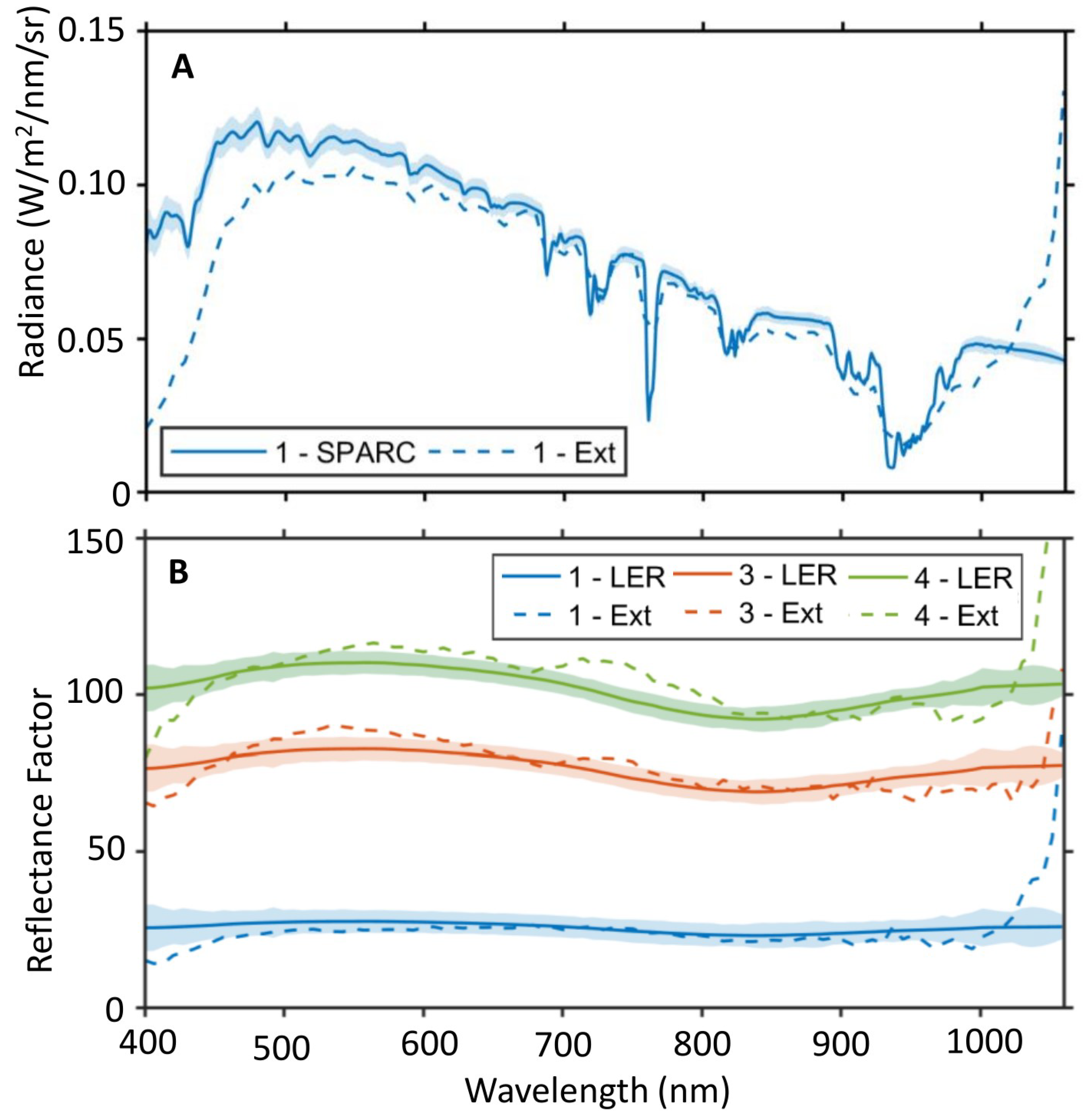
3.1. Surface Downwelling Irradiance

In-situ global downwelling solar irradiance ( E g l o ) was continuously measured over the course of the experiment. At five minute intervals during overflights, the irradiance sensor was shaded to measure the diffuse ( E d i f ) which also allows the direct ( E s ) component to be determined ( E d i f E g l o ) (Supplemental Figure S1A). Atmospheric conditions remained highly stable during the course of the experiment as determined by optical transmission (Supplemental Figure S1B), with no observable cloud cover over the target area.

3.2. Surface Reflectance Ground Truth

Reflectance of all major diffuse calibration and test targets, as well as in-scene natural targets including sand and asphalt, was measured immediately before, during, and following the overflights (Supplemental Figure S2). Spectra from each target were converted to reflectance using measurements of a 99% Spactralon® calibrated reference target. Spectra of the primary targets (5% and 50% Permaflect targets), used as potential surface reflectance targets in the application of traditional ELM processing, were acquired in close proximity to the UAV and airborne hyperspectral image acquisitions. All field reflectance measurements were performed at nadir and adjusted for SZA effects by applying an offset for Spectralon’s known divergence from true Lambertian BRDF [48].

3.3. Unmanned Aerial Vehicle Imagery

The preliminary results over the primary target area (Figure 7A) demonstrate the feasibility of mirrors for calibrating hyperspectral imagery from raw DN to surface reflectance, utilizing the UAV SPARC targets (Figure 8A). By applying Equation (3) to the mirrors with measured solar irradiance during the experiment, an LER for each of the targets (1 mirror and 2 mirrors) can be predicted (Figure 8B, solid lines). The data match, within the uncertainty of the LER, to reflectance spectra extracted from the UAV imagery (Figure 8B, dashed lines) which was calibrated using the two Permaflect® standards in the more traditional reflectance-based ELM approach.
With the exception of low instrument sensitivity and atmospheric water absorption regions near 400 and 1000 nm, the extracted reflectance spectra match the predicted LER values to within the estimated 7.20% uncertainty [63] of the predicted values. This uncertainty is a preliminary, conservative estimate based on the Root Sum Square (RSS) method [64] of the main driving factors, and is dominated by the uncertainty in GSD, a result of the accuracy of the IMU/GPS and the complex motion blur induced on the fix mounted HSI system from the UAV (Table 2). Greater accuracy in the altitude of the UAV (i.e., the IMU/GPS) and reducing motion blur in the pitch could therefore reduce the uncertainty significantly.
Notably, the magnitude of the extracted mirror surface reflectance greatly exceeds that of even the most reflective diffuse targets. Due to the specular and sub-pixel nature of the SPARC mirrors, the solar energy illuminating the sensor is directional and dispersed in pixel space across the sensor’s Point Spread Function (PSF), resulting in reflectance above 100%. Unlike with diffuse reflectance targets, the geometric properties of the mirrors allows for the relative intensity to be controlled, and high radiance targets can be displayed to an imaging system without saturation. Further studies are warranted to characterize non-linearity within the UAV instrumentation, which will impact radiometric performance over the sensor’s dynamic range. Preliminary laboratory work has indicated non-linearity in the Analog-to-Digital Conversion (ADC) gain which may account for some of the discrepancy between predicted and extracted mirror reflectance. Future experiments can be conducted with mirrors that cover the full dynamic range of the sensor and include values below 100% surface reflectance, i.e., suitable to most Earth Observation studies.

3.4. Airborne Imagery

Raw flight imagery was converted to a non-geocorrected radiance product (Level 1A) using the manufacturer provided calibration. Using the 1 mirror floating target as an example (Figure 9A), the extracted radiance is within the estimated uncertainty of the predicted at-aperture radiance (approx. 3.6%, k = 1) over the 600–975 nm range. Outside of this range (<600 nm and >975 nm), discrepancy between predicted and extracted values is observed (discussed below). The at-aperture radiance uncertainty was estimated spectrally utilizing a Monte-Carlo Method [64]. Outside of the atmospheric absorption bands and low sensitivity regions (<425 nm), the estimated relative uncertainty for at-aperture SPARC radiance was <4%, k = 1 (Table 3). Radiometric uncertainty of the SPARC LER was held equal to the at-aperture estimate for this analysis.
As with the UAV imagery, CASI imagery was calibrated to surface reflectance using the two Permaflect® standards. The LER of mirror targets was calculated (Equation (3)) and compared to the extracted surface reflectance signal from the imagery. Both the overall magnitude and shape of the extracted SPARC targets (Ext) agree with the predicted values (LER) for selected one, three, and four mirror targets (Figure 9B). It should be noted that for the one mirror floating target, agreement between predicted and retrieved spectra is within the estimated uncertainty of the measurement over most of the 450–1000 nm range. The one mirror LER, approx. 25%, is within the ELM calibrated range of the image. The three and four mirror targets (approx. 76% and 102%, respectively) fell outside of the range of the Permaflect® calibration and showed a poorer match to the predicted values. The in-scene ELM approach is not the standard procedure utilized by NRC to produce surface reflectance imagery; a method applicable to both UAV and airborne platforms was employed during this experiment.
Three notable features in the retrieved spectra are evident. Firstly, the roll-off in reflectance (and radiance) below 500 nm was anticipated, due to low sensitivity of the detector to this spectral region. Secondly, the sharp rise in reflectance above 1000 nm is believed to be the result of frame shift smear, in which the architecture of the sensor, the integration delay, and the motion of the aircraft combine to shift IR signal from a sampled pixel into subsequent along-track pixels. Lastly, the retrieved reflectance of the 3 and 4 mirror targets, which were placed on a grass and sand background in the primary target area (Figure 2), feature distinct peaks between approximately 543 and 803 nm. These features are likely due to inhomogeneity of the background reflectance. A refinement of the signal extraction and correction process to account for these effects is in development.

3.5. Satellite Imagery

The GeoEye-1 25.9° image was selected for preliminary analysis as it represents the imagery closest to nadir (Figure 7C). Selected high-quality targets were evaluated for both Level 1B Top of Atmosphere radiance and AComp corrected surface reflectance. One 6 mirror target (6B) and 2 of the 12 mirror targets (12A, B) were considered suitable for analysis. For each of the spectral bands (blue, green, red, NIR), the majority of the Level 1B extracted data points agreed to the SPARC predicted values (Figure 10A) within the uncertainty of the measurements. SPARC at-aperture radiance and LER uncertainty was estimated to be equal to that for the airborne instrumentation (Table 3). For target 12A, the retrieved radiance was significantly lower than the SPARC radiance in the green channel, while a similar phenomenon was observed in the NIR band for target 12B. Target 6B data could not be extracted for the NIR band.
In contrast to the Level 1B radiance data, there is a strong absolute bias and spectral shape in the retrieved surface reflectance of the SPARC targets in AComp imagery, relative to the predicted LER (Figure 10B). This bias is not observed in either the Level 1B data, or in the AComp retrieved reflectance of large homogeneous targets (Figure 11).

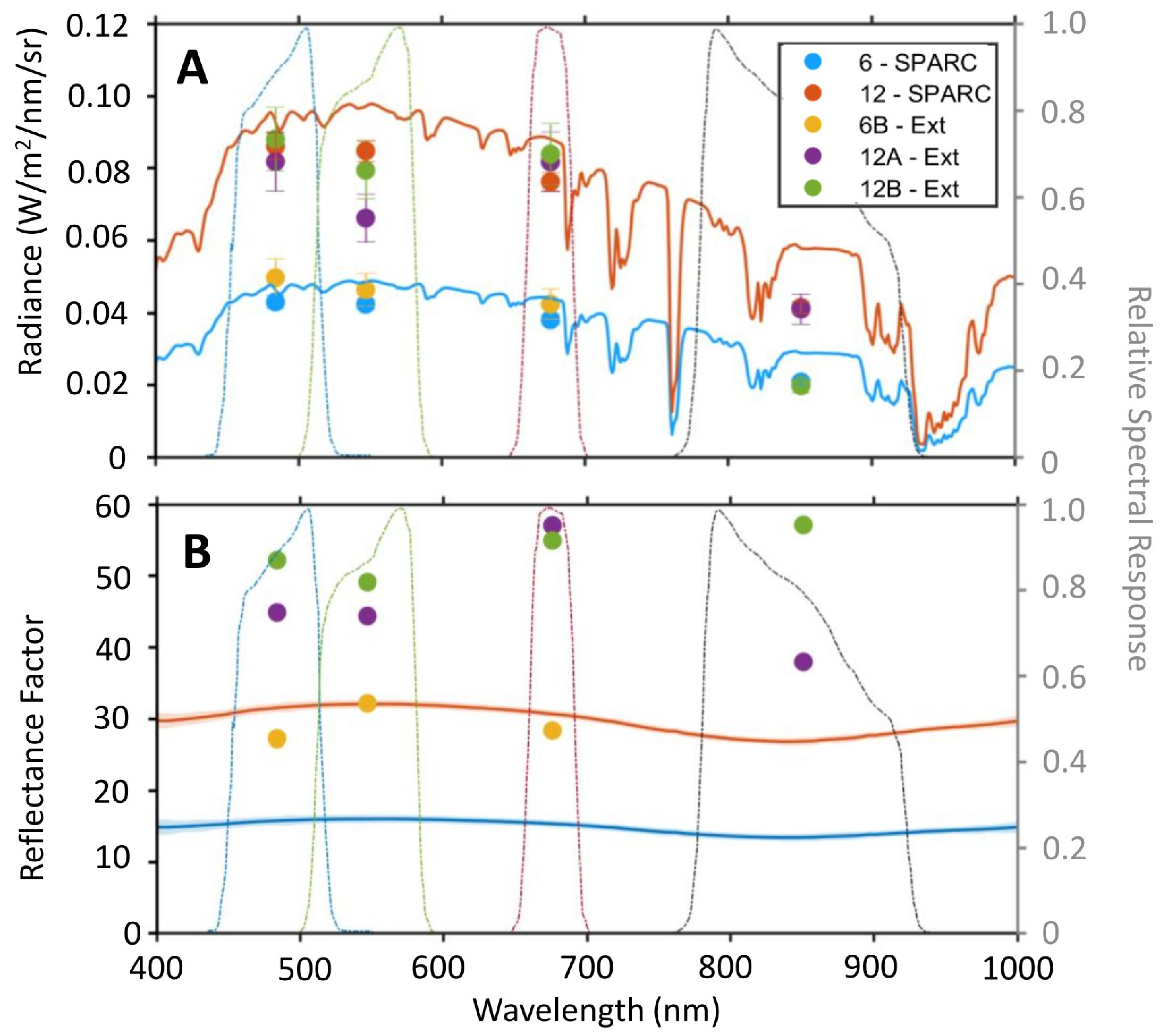
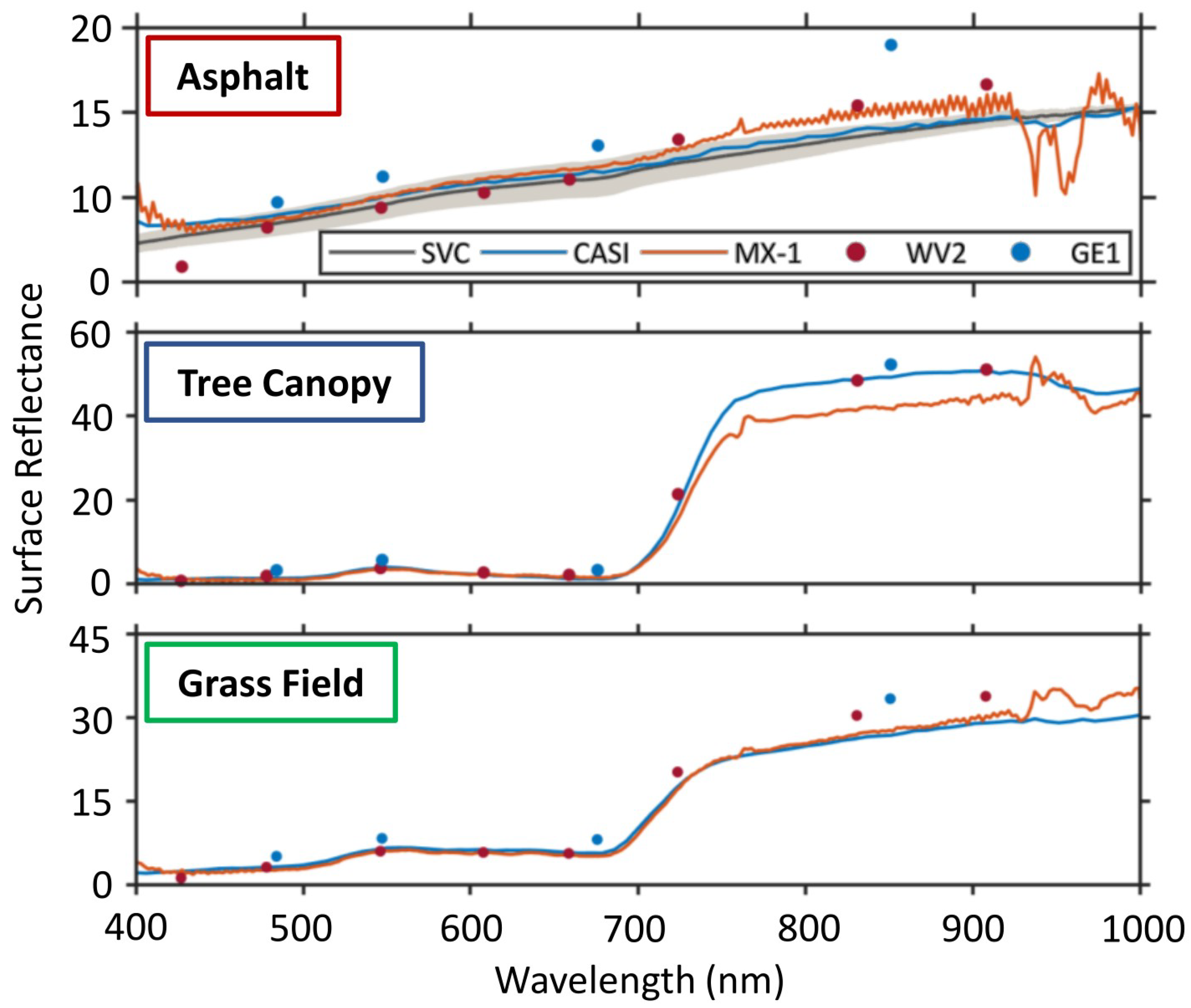
3.6. Cross-Platform Surface Reflectance Retrieval

Within the main test area imaged by all assets, Large Areas of Interest (AOIs) were extracted from a test image from each platform for comparison (Figure 7A) across tree canopy (blue), asphalt (red), and grass field (green) AOIs. The reflectance of the asphalt AOI target (Figure 11) was measured with the SVC following the overflights. Airborne, UAV, and WV2 retrieved surface reflectance agree, over most of the visible wavelengths, within the variation of the ground measurements. For all AOIs, surface reflectance retrievals agree in magnitude and spectral shape across platforms. Some discrepancies are evident between airborne and UAV platforms due to collection methodologies. To a first order, satellite retrievals agree well to the other sensors. Differences are potentially explained by the impacts of the Bidirectional Reflectance Distribution Function (BRDF) of the AOI targets themselves. While UAV and airborne sensors viewed the scene from a similar nadir and azimuthal geometry, satellite platforms imaged the experimental area from up to 30° off nadir and a variable azimuth. The impact of these discrepancies on surface retrievals will be the subject of future study. Secondly, while the AComp correction methodology has been thoroughly validated and the Maxar calibration methods are based on a similar ELM method, AComp represents a generic global approach which cannot represent the highest accuracy atmospheric correction for a given instance.
The diffuse reflectance calibration and validation targets deployed during the G-SCALE were sized specifically for the GSDs of airborne and UAV sensors. While visible and recognizable in satellite imagery (Figure 7C), none of these targets were sufficiently sized to present radiometrically accurate pixels to WorldView-2 or GeoEye-1 multispectral channels. This prevents a simultaneous intercalibration of all platforms to surface reflectance using traditional calibration approaches. By contrast to diffuse targets, the SPARC mirrors deployed during G-SCALE were tailored to all asset classes. Using the MELM approach (Equation (4)), the retrieved surface reflectance of each AOI could be simultaneously calibrated using in-scene data, potentially improving cross-platform agreement.

4. Conclusions

Data harmonization and interoperability between remote sensing platforms will be key to enabling the potential of current and future Earth Observation missions. The challenges of ensuring consistent data quality between products at different spatial, temporal, and spectral resolutions will require innovative cal/val methods and technologies as well as automated and scalable data flows. The SPARC method represents one such tool, particularly if utilized in an automated and accessible network [45]. A number of studies utilizing the G-SCALE data set are currently in progress. Preliminary results using traditional diffuse reflectance calibration methods yielded good agreement between UAV and airborne platforms, as well as a first order agreement to satellite retrievals with bias that could be attributed to target BRDF, viewing geometry, and atmospheric correction routines. Diffuse ELM calibration of hyperspectral imagery retrieved SPARC-based Lambertian Equivalent Reflectance to within the uncertainty of the measurement. Airborne CASI data, calibrated to absolute radiance with a NIST traceable integrating sphere, agreed with the SPARC target projected radiance at higher levels while showing a negative bias at lower levels. Both these results and previous studies [35] demonstrate the utility of floating SPARC targets for remote sensing of water-based targets. This paper has focused primarily on the VISNIR spectral range (400–1000 nm) due to commonality between all platforms. However, irradiance, surface reflectance, airborne, and UAV data sets extend to the SWIR wavelengths, with commonality to 2200 nm. An analysis of platform intercalibration using SPARC at longer wavelengths is forthcoming. Comparisons of surface reflectance and radiance products derived using diffuse and specular calibration is being conducted for all sensor platforms, as well as investigation of potential biases in retrieval across asset classes.
For constellations of numerous sensors, it is necessary to monitor radiometric performance year-round. A winter-suitable method, such as the SPARC technique as employed by the Field Line-of-sight Radiometric Exposure (FLARE) Network [45], would allow for monitoring of sensor performance throughout conditions when it is not viable to deploy the calibration tarps. If the additional calibration system can be tied to the primary system and shown to be stable, then that system can be used with confidence in the off-season for sensor monitoring. For cross calibration of EO sensors, knowledge of the hyperspectral reflectance of targets being utilized is required. Often there is a bias of the target itself that can seep into the results, especially if the target is spectrally non-homogenous over the regions of interest or has geometric dependencies (BRDF). The reflectance of the mirrors and mounting material would be well known and identical for multiple calibration sites, thus removing the bias inherent to differing natural targets. In addition, it is often difficult to collect simultaneous imagery among sensors using only one site. A set of nationally or globally distributed FLARE stations could facilitate cross-calibration campaigns within a single operator’s constellations, and to offer consistent traceable calibrations to other commercial and government EO sensors, aircraft, and UAV sensors so that this imagery may be used in concert for scientific remote sensing. Previous experiments with Maxar’s WorldView-3 satellite and the SPARC technique have revealed excellent agreement in Top of Atmosphere Radiance of mirror targets, as well as the Railroad Valley Playa RadCalNet site (Supplemental Figure S3).
Understanding the differences in the absolute radiometric performance of a sensor with respect to variation in GSD is important for agile sensors capable of pointing and highly off-nadir viewing geometries, or for push-broom style sensors operating at varying ground-speed. Variation in GSD and image quality metrics can differ across nominally identical sensors as well, and an inter-calibration method is required. This campaign starts a discussion for understanding how sensor radiometric response may differ spatially.
Of particular interest is the discrepancy between predicted and retrieved Lambertian Equivalent Reflectance for the mirror targets in GeoEye-1 imagery (Figure 10B). Good agreement was observed for the SPARC targets at the Level 1B radiance level (Figure 10A), and comparable reflectance was observed for asphalt, tree, and grass ROIs across all sensors (Figure 11). While the reasons behind this discrepancy are under investigation, this result demonstrates the utility of calibration with mirror-based point targets for accurate small-target radiometry. In fact, the SPARC mirrors provide a uniquely powerful tool for evaluating the radiometric and geospatial impacts of resampling and processing at each image product level. Exploiting SPARC for small-target and alternative calibration techniques is the subject of active collaborative research by the authors.
Due to inhomogeneity of the background reflectance and the viewing geometry at time of collect, not all SPARC targets visible in the imagery were considered suitable for radiometric analysis. This highlights the importance of target location, mirror selection, and pointing accuracy to successful application of the SPARC methodology. In fact, SPARC has been utilized to great effect with Maxar assets in previous studies. Surface reflectance calibration of Level 1 Worldview-2 imagery using the MELM method [46] demonstrated high-fidelity to in-situ measurements, and Top of Atmosphere radiance calibration of Worldview-3 (Supplemental Figure S3) agreed with surface validation measurements to within the measurement uncertainty. Refinement of the SPARC retrievals during G-SCALE will be the subject of ongoing efforts.
In addition to Maxar assets, there was a concurrent collection by Landsat 8 of the area including Tait Preserve (Supplemental Figure S4) (15:51 UTC). No SPARC targets were deployed suitable for calibration of the Landsat 8 OLI 30 m pixels during the G-SCALE. However, a transfer calibration can potentially be applied from the higher resolution GeoEye-1 and WorldView-2 imagery to the Landsat 8 data using larger objects in-scene. It should be noted that two of the automated SPARC targets employed by the FLARE Network are optimized for 10–60 m GSDs [45], and are currently being investigated to directly validate Top of Atmosphere radiance for Landsat 8/9 OLI and Sentinel 2A/B MSI imagery using the SPARC method.
An important, and less tangible, aspect of intercalibration exercises is the exchange and comparison of expertise, knowledge and methodologies among participating groups. This type of experiment therefore yields benefits to the broader Earth Observation remote sensing community. For example, retrieved MX-1 surface reflectance in the NIR shows substantial artifacts associated with atmospheric water vapor absorption centered around 940 nm and the 760 nm oxygen A-band (Figure 11) which are not evident in the CASI data, though both were calibrated using the in-scene Permaflect® panels. It was determined that the large swath of the airborne imagery, which covered the entire experimental area, allowed for the collection of both panels and all targets almost simultaneously, minimizing the impact of short-term atmospheric variation for a given single flight line. By contrast, the raster approach of the UAV survey resulted in a significant delay (up to 20 min) between the beginning and end of an imagery collection containing all necessary AOIs and calibration targets. This has led to a subsequent modification in UAV operations to include more frequent imaging of reference targets during field operations.
One of the potential advantages of SPARC targets for calibration and validation is that they are significantly smaller and easier to deploy relative to large reflectance targets which must be many times the GSD of the sensor under test. Mirror sets can be easily deployed, in the same general area, for sensors with GSDs between <10 cm to 2 m (this study) or larger [45]. Mirrors can also be deployed in difficult or heterogenous environments with dynamic atmospheres and low signal radiance, such as large bodies of water, where traditional calibration methodologies may not be suitable. With the ability to tune specular targets for multiple radiance (or Lambertian Equivalent Reflectance) levels, the Mirror-based Empirical Line Method (MELM) can be applied over the dynamic range of the instrument. Such a calibration technique could be of particular importance in spectral regions or signal strength ranges where a sensor’s response is non-linear. It should be noted that while the primary goal of the G-SCALE was radiometric and reflectance calibration and characterization, the spatial performance of an imaging sensor is critical to data quality and suitability for a given EO task. The point-source nature of SPARC targets allows them to be used to generate spatial and image quality metrics like MTF or Rayleigh Criteria. Comparison of SPARC-based spatial metrics with those derived from edge targets during this experiment will be the topic of future studies.

Supplementary Materials

The following supporting information can be downloaded at: https://www.mdpi.com/article/10.3390/rs15020294/s1, Figure S1: Solar and atmospheric conditions during the G-SCALE; Figure S2: Diffuse target reflectance; Figure S3: SPARC and WorldView-3 radiance; Figure S4: Landsat 8 imagery during the G-SCALE; Table S1: Key characteristics of the NRC operated CASI-1500 and SASI-600 Airborne Hyperspectral Systems.

Author Contributions

Conceptualization, B.J.R., E.J.I. and C.D.; methodology, B.J.R., R.J.S., J.P.A.-M., E.J.I. and D.N.C.; data acquisition, B.J.R., R.J.S., D.N.C., M.A.K., T.O. and C.D.; image processing, J.H.; formal analysis, B.J.R.; data curation, B.J.R., J.H., D.N.C. and E.J.I.; writing—original draft preparation, B.J.R., R.J.S., E.J.I., D.N.C. and M.A.K.; writing—review and editing, B.J.R., J.P.A.-M., T.O., C.D. and J.H.; funding acquisition, E.J.I., J.P.A.-M. and C.D. All authors have read and agreed to the published version of the manuscript.

Funding

Deployment of SPARC mirrors and Permaflect standards was funded through a Labsphere internal development budget. UAV survey and ground reflectance measurements were funded jointly by Labsphere and author EI discretionary funds through RIT. Satellite imagery provided by Maxar calibration efforts. Airborne imagery collection and analysis was funded internally by NRC.

Data Availability Statement

The data presented in this study are available on request from the corresponding author.

Acknowledgments

The authors wish to thank Nina Raqueno and Tim Bauch of RIT for collection of ground reflectance spectra and UAV operations. The contributions to the successful acquisition of the airborne hyperspectral imagery of pilot Reagh Sherwood, flight engineer Peter Earle, aircraft mechanic Kevin Cahill, and instrumentation support by Ahsan Aziz are gratefully acknowledged. We thank Stephen Schiller of Raytheon Space and Airborne Systems for comments and suggestions on the manuscript.

Conflicts of Interest

Authors B.J.R., C.D. and J.H. are employed by Labsphere, Inc. which has a commercial interest in calibration and validation technologies, including Lambertian and specular materials and techniques. Authors M.A.K. and T.O. are employed by Maxar, Inc. which has a commercial interest in providing satellite imagery to private and government sources. Funding for the collection of data was provided by internal money from each group responsible for that data. No external funding was received. Analysis of imagery was performed independently of commercial source providers to ensure impartiality.

References

  1. Kansakar, P.; Hossain, F. A review of applications of satellite earth observation data for global societal benefit and stewardship of planet earth. Space Policy 2016, 36, 46–54. [Google Scholar] [CrossRef]
  2. Rice, K. Convolutional Neural Networks for Detection and Classification of Maritime Vessels in Eletro-Optical Satellite Imagery. Ph.D. Thesis, Naval Postgraduate School, Monterey, CA, USA, 2018. [Google Scholar]
  3. Agapiou, A. Evaluation of Landsat 8 OLI/TIRS Level-2 and Sentinel 2 Level-1C Fusion Techniques Intended for Image Segmentation of Archaeological Landscapes and Proxies. Remote Sens. 2020, 12, 579. [Google Scholar] [CrossRef] [Green Version]
  4. Niroumand-Jadidi, M.; Bovolo, F.; Bruzzone, L.; Gege, P. Physics-based Bathymetry and Water Quality Retrieval Using PlanetScope Imagery: Impacts of 2020 COVID-19 Lockdown and 2019 Extreme Flood in the Venice Lagoon. Remote Sens. 2020, 12, 2381. [Google Scholar] [CrossRef]
  5. Ustin, S.L.; Middleton, E.M. Current and near-term advances in Earth observation for ecological applications. Ecol. Process. 2021, 10, 1. [Google Scholar] [CrossRef] [PubMed]
  6. Yao, H.; Qin, R.; Chen, X. Unmanned Aerial Vehicle for Remote Sensing Applications—A Review. Remote Sens. 2019, 11, 22. [Google Scholar] [CrossRef] [Green Version]
  7. Zhang, H.; Wang, L.; Tian, T.; Yin, J. A Review of Unmanned Aerial Vehicle Low-Altitude Remote Sensing (UAV-LARS) Use in Agricultural Monitoring in China. Remote Sens. 2021, 13, 17. [Google Scholar] [CrossRef]
  8. Akumu, C.E.; Amadi, E.O.; Dennis, S. Application of Drone and WorldView-4 Satellite Data in Mapping and Monitoring Grazing Land Cover and Pasture Quality: Pre- and Post-Flooding. Land 2021, 10, 321. [Google Scholar] [CrossRef]
  9. Backes, D.J.; Teferle, F.N. Multiscale Integration of High-Resolution Spaceborne and Drone-Based Imagery for a High-Accuracy Digital Elevation Model Over Tristan da Cunha. Front. Earth Sci. 2020, 8, 319. [Google Scholar] [CrossRef]
  10. Bracaglia, M.; Santoleri, R.; Volpe, G.; Colella, S.; Benincasa, M.; Brando, V.E. A Virtual Geostationary Ocean Color Sensor to Analyze the Coastal Optical Variability. Remote Sens. 2020, 12, 1539. [Google Scholar] [CrossRef]
  11. Claverie, M.; Ju, J.; Masek, J.G.; Dungan, J.L.; Vermote, E.F.; Roger, J.C.; Skakun, S.V.; Justice, C. The Harmonized Landsat and Sentinel-2 surface reflectance data set. Remote Sens. Environ. 2018, 219, 145–161. [Google Scholar] [CrossRef]
  12. Hegarty-Craver, M.; Polly, J.; O’Neil, M.; Ujeneza, N.; Rineer, J.; Beach, R.H.; Lapidus, D.; Temple, D.S. Remote Crop Mapping at Scale: Using Satellite Imagery and UAV-Acquired Data as Ground Truth. Remote Sens. 2020, 12, 1984. [Google Scholar] [CrossRef]
  13. Kopp, S.; Becker, P.; Doshi, A.; Wright, D.J.; Zhang, K.; Xu, H. Achieving the Full Vision of Earth Observation Data Cubes. Data 2019, 4, 94. [Google Scholar] [CrossRef] [Green Version]
  14. Maritorena, S.; d’ Andon, O.H.F.; Mangin, A.; Siegel, D.A. Merged satellite ocean color data products using a bio-optical model: Characteristics, benefits and issues. Remote Sens. Environ. 2010, 114, 1791–1804. [Google Scholar] [CrossRef]
  15. Mazzia, V.; Comba, L.; Khaliq, A.; Chiaberge, M.; Gay, P. UAV and Machine Learning Based Refinement of a Satellite-Driven Vegetation Index for Precision Agriculture. Sensors 2020, 20, 2530. [Google Scholar] [CrossRef]
  16. Nikolakopoulos, K.; Kyriou, A.; Koukouvelas, I.; Zygouri, V.; Apostolopoulos, D. Combination of Aerial, Satellite, and UAV Photogrammetry for Mapping the Diachronic Coastline Evolution: The Case of Lefkada Island. ISPRS Int. J. Geo-Inf. 2019, 8, 489. [Google Scholar] [CrossRef] [Green Version]
  17. Niro, F.; Goryl, P.; Dransfeld, S.; Boccia, V.; Gascon, F.; Adams, J.; Themann, B.; Scifoni, S.; Doxani, G. European Space Agency (ESA) Calibration/Validation Strategy for Optical Land-Imaging Satellites and Pathway towards Interoperability. Remote Sens. 2021, 13, 3003. [Google Scholar] [CrossRef]
  18. Sogacheva, L.; Popp, T.; Sayer, A.M.; Dubovik, O.; Garay, M.J.; Heckel, A.; Hsu, N.C.; Jethva, H.; Kahn, R.A.; Kolmonen, P.; et al. Merging Regional and Global AOD Records from 15 Available Satellite Products; Technical Report; European Geosciences Union: Munich, Germany, 2019; Available online: https://acp.copernicus.org/articles/20/2031/2020/ (accessed on 11 November 2022). [CrossRef]
  19. Szantoi, Z.; Geller, G.N.; Tsendbazar, N.E.; See, L.; Griffiths, P.; Fritz, S.; Gong, P.; Herold, M.; Mora, B.; Obregon, A. Addressing the need for improved land cover map products for policy support. Environ. Sci. Policy 2020, 112, 28–35. [Google Scholar] [CrossRef]
  20. Kang, J.; Jin, R.; Li, X. An Advanced Framework for Merging Remotely Sensed Soil Moisture Products at the Regional Scale Supported by Error Structure Analysis: A Case Study on the Tibetan Plateau. IEEE J. Sel. Top. Appl. Earth Obs. Remote Sens. 2021, 14, 3614–3624. [Google Scholar] [CrossRef]
  21. Mélin, F.; Sclep, G.; Jackson, T.; Sathyendranath, S. Uncertainty estimates of remote sensing reflectance derived from comparison of ocean color satellite data sets. Remote Sens. Environ. 2016, 177, 107–124. [Google Scholar] [CrossRef]
  22. Shen, Y.; Xiong, A.; Hong, Y.; Yu, J.; Pan, Y.; Chen, Z.; Saharia, M. Uncertainty analysis of five satellite-based precipitation products and evaluation of three optimally merged multi-algorithm products over the Tibetan Plateau. Int. J. Remote Sens. 2014, 35, 6843–6858. [Google Scholar] [CrossRef]
  23. Bouvet, M.; Thome, K.; Berthelot, B.; Bialek, A.; Czapla-Myers, J.; Fox, N.P.; Goryl, P.; Henry, P.; Ma, L.; Marcq, S.; et al. RadCalNet: A Radiometric Calibration Network for Earth Observing Imagers Operating in the Visible to Shortwave Infrared Spectral Range. Remote Sens. 2019, 11, 2401. [Google Scholar] [CrossRef] [Green Version]
  24. Helder, D.; Anderson, C.; Beckett, K.; Houborg, R.; Zuleta, I.; Boccia, V.; Clerc, S.; Kuester, M.; Markham, B.; Pagnutti, M. Observations and Recommendations for Coordinated Calibration Activities of Government and Commercial Optical Satellite Systems. Remote Sens. 2020, 12, 2468. [Google Scholar] [CrossRef]
  25. Huang, H.; Roy, D. Characterization of Planetscope-0 Planetscope-1 surface reflectance and normalized difference vegetation index continuity. Sci. Remote Sens. 2021, 3, 100014. [Google Scholar] [CrossRef]
  26. Lewis, A.; Lacey, J.; Mecklenburg, S.; Ross, J.; Siqueira, A.; Killough, B.; Szantoi, Z.; Tadono, T.; Rosenavist, A.; Goryl, P.; et al. CEOS Analysis Ready Data for Land (CARD4L) Overview. In Proceedings of the IGARSS 2018—2018 IEEE International Geoscience and Remote Sensing Symposium, Valencia, Spain, 22–27 July 2018; pp. 7407–7410. [Google Scholar] [CrossRef]
  27. Manivasagam, V.; Kaplan, G.; Rozenstein, O. Developing Transformation Functions for VENUS and Sentinel-2 Surface Reflectance over Israel. Remote Sens. 2019, 11, 1710. [Google Scholar] [CrossRef] [Green Version]
  28. Shrestha, M.; Hasan, N.; Leigh, L.; Helder, D. Derivation of Hyperspectral Profile of Extended Pseudo Invariant Calibration Sites (EPICS) for Use in Sensor Calibration. Remote Sens. 2019, 11, 2279. [Google Scholar] [CrossRef] [Green Version]
  29. Siqueira, A.; Lewis, A.; Thankappan, M.; Szantoi, Z.; Goryl, P.; Labahn, S.; Ross, J.; Hosford, S.; Mecklenburg, S.; Tadono, T.; et al. CEOS Analysis Ready Data For Land—An Overview on the Current and Future Work. In Proceedings of the IGARSS 2019—2019 IEEE International Geoscience and Remote Sensing Symposium, Yokohama, Japan, 28 July–2 August 2019; pp. 5536–5537. [Google Scholar] [CrossRef]
  30. Le Roux, J.; Christopher, S.; Maskey, M. Exploring the Use of PlanetScope Data for Particulate Matter Air Quality Research. Remote Sens. 2021, 13, 2981. [Google Scholar] [CrossRef]
  31. Bruegge, C.J.; Crisp, D.; Helmlinger, M.C.; Kataoka, F.; Kuze, A.; Lee, R.A.; McDuffie, J.L.; Rosenberg, R.A.; Schwandner, F.M.; Shiomi, K.; et al. Vicarious Calibration of Orbiting Carbon Observatory-2. IEEE Trans. Geosci. Remote Sens. 2019, 57, 5135–5145. [Google Scholar] [CrossRef]
  32. Kuze, A.; O’Brien, D.M.; Taylor, T.E.; Day, J.O.; O’Dell, C.W.; Kataoka, F.; Yoshida, M.; Mitomi, Y.; Bruegge, C.J.; Pollock, H.; et al. Vicarious Calibration of the GOSAT Sensors Using the Railroad Valley Desert Playa. IEEE Trans. Geosci. Remote Sens. 2011, 49, 1781–1795. [Google Scholar] [CrossRef]
  33. Sterckx, S.; Wolters, E. Radiometric Top-of-Atmosphere Reflectance Consistency Assessment for Landsat 8/OLI, Sentinel-2/MSI, PROBA-V, and DEIMOS-1 over Libya-4 and RadCalNet Calibration Sites. Remote Sens. 2019, 11, 2253. [Google Scholar] [CrossRef] [Green Version]
  34. Jin, C.; Ahn, H.; Seo, D.; Choi, C. Radiometric Calibration and Uncertainty Analysis of KOMPSAT-3A Using the Reflectance-Based Method. Sensors 2020, 20, 2564. [Google Scholar] [CrossRef]
  35. Ortiz, J.D.; Avouris, D.; Schiller, S.; Luvall, J.C.; Lekki, J.D.; Tokars, R.P.; Anderson, R.C.; Shuchman, R.; Sayers, M.; Becker, R. Intercomparison of Approaches to the Empirical Line Method for Vicarious Hyperspectral Reflectance Calibration. Front. Mar. Sci. 2017, 4, 296. [Google Scholar] [CrossRef] [Green Version]
  36. Minařík, R.; Langhammer, J.; Hanuš, J. Radiometric and Atmospheric Corrections of Multispectral micro-MCA Camera for UAV Spectroscopy. Remote Sens. 2019, 11, 2428. [Google Scholar] [CrossRef] [Green Version]
  37. Smith, G.M.; Milton, E.J. The use of the empirical line method to calibrate remotely sensed data to reflectance. Int. J. Remote Sens. 1999, 20, 2653–2662. [Google Scholar] [CrossRef]
  38. Languille, F.; Déchoz, C.; Gaudel, A.; Greslou, D.; de Lussy, F.; Trémas, T.; Poulain, V. Sentinel-2 geometric image quality commissioning: First results. In Image and Signal Processing for Remote Sensing XXI; Bruzzone, L., Ed.; SPIE Remote Sensing: Toulouse, France, 2015; p. 964306. [Google Scholar] [CrossRef]
  39. Pandžić, M.; Mihajlovic, D.; Pandžić, J.; Pfeifer, N. Assessment of the geometric quality of sentinel-2 data. Int. Arch. Photogramm. Remote Sens. Spat. Inf. Sci. 2016, XLI-B1, 489–494. [Google Scholar] [CrossRef] [Green Version]
  40. Wenny, B.; Helder, D.; Hong, J.; Leigh, L.; Thome, K.; Reuter, D. Pre- and Post-Launch Spatial Quality of the Landsat 8 Thermal Infrared Sensor. Remote Sens. 2015, 7, 1962–1980. [Google Scholar] [CrossRef] [Green Version]
  41. Shrestha, M.; Hasan, M.N.; Leigh, L.; Helder, D. Extended Pseudo Invariant Calibration Sites (EPICS) for the Cross-Calibration of Optical Satellite Sensors. Remote Sens. 2019, 11, 1676. [Google Scholar] [CrossRef]
  42. Schiller, S.J.; Silny, J. The Specular Array Radiometric Calibration (SPARC) method: A new approach for absolute vicarious calibration in the solar reflective spectrum. In Remote Sensing System Engineering III; Ardanuy, P.E., Puschell, J.J., Eds.; SPIE Optical Engineering + Applications: San Diego, CA, USA, 2010; Volume 7813, p. 78130E. [Google Scholar] [CrossRef]
  43. Schiller, S.J.; Teter, M.; Silny, J. Comprehensive vicarious calibration and characterization of a small satellite constellation using the Specular ARray Calibration (SPARC) method. In Proceedings of the Session 6: Science Mission Payloads 1, Logan, UT, USA, 10 August 2017; p. 12. [Google Scholar]
  44. Schiller, S.; Silny, J. Using vicarious calibration to evaluate small target radiometry. In Proceedings of the Calcon 2016; 25th Annual Meeting on Characterization and Radiometric Calibration for Remote Sensing, Logan, UT, USA, 25 August 2016; p. 1. [Google Scholar]
  45. Russell, B.; Scharpf, D.; Holt, J.; Arnold, W.; Durell, C.N.; Jablonski, J.; Conran, D.; Schiller, S.J.; Leigh, L.; Aaron, D.; et al. Initial results of the FLARE vicarious calibration network. In Earth Observing Systems XXV; Butler, J.J., Xiong, X.J., Gu, X., Eds.; SPIE: Online Only, 2020; p. 14. [Google Scholar] [CrossRef]
  46. Schiller, S.J. Demonstration of the Mirror-based Empirical Line Method (MELM). In Proceedings of the 18th Annual Joint Agency Commercial Imagery Evaluation (JACIE) Workshop, Reston, VA, USA, 24 September 2019; p. 12. [Google Scholar]
  47. Joseph, G. Fundamentals of Remote Sensing, 2nd ed; Universities Press (India) Private Limited: Hyderabad, India, 2005. [Google Scholar]
  48. Soffer, R.J.; Ifimov, G.; Arroyo-Mora, J.P.; Kalacska, M. Validation of Airborne Hyperspectral Imagery from Panel Characterization to Image Quality Assessment Implications for an Arctic Peatland Surrogate Simulation Site Laboratory. Can. J. Remote Sens. 2019, 45, 476. [Google Scholar] [CrossRef]
  49. Herweg, J.A.; Kerekes, J.P.; Weatherbee, O.; Messinger, D.; van Aardt, J.; Ientilucci, E.; Ninkov, Z.; Faulring, J.; Raqueño, N.; Meola, J. SpecTIR hyperspectral airborne Rochester experiment data collection campaign. In Algorithms and Technologies for Multispectral, Hyperspectral, and Ultraspectral Imagery XVIII; Shen, S.S., Lewis, P.E., Eds.; International Society for Optics and Photonics, SPIE: Baltimore, MD, USA, 2012; Volume 8390, pp. 717–726. [Google Scholar] [CrossRef]
  50. Giannandrea, A.; Raqueno, N.; Messinger, D.W.; Faulring, J.; Kerekes, J.P.; van Aardt, J.; Canham, K.; Hagstrom, S.; Ontiveros, E.; Gerace, A.; et al. The SHARE 2012 data campaign. In Algorithms and Technologies for Multispectral, Hyperspectral, and Ultraspectral Imagery XIX; Shen, S.S., Lewis, P.E., Eds.; International Society for Optics and Photonics, SPIE: Baltimore, MD, USA, 2013; Volume 8743, pp. 94–108. [Google Scholar] [CrossRef]
  51. Ientilucci, E.J. SHARE 2012: Analysis of illumination differences on targets in hyperspectral imagery. In Algorithms and Technologies for Multispectral, Hyperspectral, and Ultraspectral Imagery XIX; Shen, S.S., Lewis, P.E., Eds.; International Society for Optics and Photonics, SPIE: Baltimore, MD, USA, 2013; Volume 8743, pp. 125–136. [Google Scholar] [CrossRef]
  52. Ientilucci, E.J. Using a new GUI tool to leverage LiDAR data to aid in hyperspectral image material detection in the radiance domain on RIT SHARE LiDAR/HSI data. In Imaging Spectrometry XVIII; Mouroulis, P., Pagano, T.S., Eds.; International Society for Optics and Photonics, SPIE: San Diego, CA, USA, 2013; Volume 8870, pp. 57–67. [Google Scholar] [CrossRef]
  53. Ientilucci, E.J. Target detection assessment of the SHARE 2010/2012 hyperspectral data collection campaign. In Algorithms and Technologies for Multispectral, Hyperspectral, and Ultraspectral Imagery XXI; Velez-Reyes, M., Kruse, F.A., Eds.; International Society for Optics and Photonics, SPIE: Baltimore, MD, USA, 2015; Volume 9472, pp. 171–181. [Google Scholar] [CrossRef]
  54. Ientilucci, E.J. New SHARE 2010 HSI-LiDAR dataset: Re-calibration, detection assessment and delivery. In Imaging Spectrometry XXI; Silny, J.F., Ientilucci, E.J., Eds.; International Society for Optics and Photonics, SPIE: San Diego, CA, USA, 2016; Volume 9976, pp. 121–129. [Google Scholar] [CrossRef]
  55. Kalacska, M.; Arroyo-Mora, J.P.; Soffer, R.; Leblanc, G. Quality Control Assessment of the Mission Airborne Carbon 13 (MAC-13) Hyperspectral Imagery from Costa Rica. Can. J. Remote Sens. 2016, 42, 85–105. [Google Scholar] [CrossRef]
  56. ITRES Research Limited. CASI Instrument Manual; ITRES Research Limited: Calgary, AB, Canada, 2008. [Google Scholar]
  57. Soffer, R. Hyperspectral Reflectance in Support of Biomass Monitoring of Agricultural Fields—Part 1: Image Georectification Support; AAFC Contract No. 3000362053; Agriculture and Agri-Food Canada: Ottawa, ON, Canada, 2008.
  58. Jia, G.; Hueni, A.; Schaepman, M.; Zhao, H. Detection and Correction of Spectral Shift Effects for the Airborne Prism Experiment. IEEE Trans. Geosci. Remote Sens. 2017, 55, 6666. [Google Scholar] [CrossRef]
  59. Chapman, J.; Thompson, D.; Helmlinger, M.; Bue, B.; Green, R.; Eastwood, M.; Geier, S.; Olson-Duvall, W.; Lundeen, S. Spectral and Radiometric Calibration of the Next Generation Airborne Visible Infrared Spectrometer (AVIRIS-NG). Remote Sens. 2019, 11, 2129. [Google Scholar] [CrossRef] [Green Version]
  60. Soffer, R.; Ifimov, G.; Pan, Y.; Belanger, S. Acquisition and Spectroradiometric Assessment of the Novel WaterSat Imaging Spectrometer Experiment (WISE) Sensor for the Mapping of Optically Shallow Coastal Waters. In Proceedings of the Hyperspectral Imaging and Sounding of the Environment 2021, Washington, DC, USA, 19–23 July 2021; The Optical Society of America: Washington, DC, USA, 2021; p. HF4E.4. [Google Scholar]
  61. Czapla-Myers, J.; McCorkel, J.; Anderson, N.; Thome, K.; Biggar, S.; Helder, D.; Aaron, D.; Leigh, L.; Mishra, N. The Ground-Based Absolute Radiometric Calibration of Landsat 8 OLI. Remote Sens. 2015, 7, 600–626. [Google Scholar] [CrossRef] [Green Version]
  62. Pacifici, F. Validation of the DigitalGlobe surface reflectance product. In Proceedings of the 2016 IEEE International Geoscience and Remote Sensing Symposium (IGARSS), Beijing, China, 10–15 July 2016; pp. 1973–1975. [Google Scholar] [CrossRef]
  63. Conran, D.; Ientilucci, E.J. Interrogating UAV Image and Data Quality Using Convex Mirrors. In Proceedings of the IGARSS 2022—2022 IEEE International Geoscience and Remote Sensing Symposium, Kuala Lumpur, Malaysia, 17–22 July 2022; pp. 4525–4528. [Google Scholar] [CrossRef]
  64. Pinto, C.T. Uncertainty Evaluation for In-Flight Radiometric Calibration of Earth Observation Sensors. Ph.D. Thesis, Instituto Nacional de Pesquisas Espaciais (INPE), San Jose Dos Campos, Brazil, 2016. [Google Scholar]
Figure 1. Study site as imaged by the airborne sensor (pseudo-RGB). Diffuse reflectance targets and calibration standards, as well as SPARC mirror targets, are visible in the primary target area (red square). Additional SPARC targets configured for satellite (yellow square) and airborne (orange circle) sensors were deployed in other locations around the study site.
Remotesensing 15 00294 g001
Figure 2. Primary target area during the G-SCALE. SPARC mirror targets for airborne and satellite assets (top inset, 0.22 m diam., 0.38 m RoC) are circled and labeled with the number of individual mirrors deployed (1–12) for that target, with additional arrays of 6 and 12 mirrors positioned North of the main area. A separate type of SPARC target was dedicated to the UAV sensors (bottom inset, left/right: 0.025 m diam., 0.05 m RoC; bottom: 0.05 m diam, 0.10 m RoC). Greyscale and colored diffuse reflectance targets are also visible.
Remotesensing 15 00294 g002
Figure 3. Floating SPARC targets (orange circles) deployed for MELM calibration of the airborne sensor at low signal levels appropriate to water-leaving radiance (Lw).
Remotesensing 15 00294 g003
Figure 4. Permaflect® reflectance standards. 50% reflectance standard (top) and 5% standard (middle) with lab measured reflectance factor (right). A green target detection panel is visible between the targets (bottom).
Remotesensing 15 00294 g004
Figure 5. Reflective targets deployed during the G-SCALE included a long, spectrally flat tarp that was used to assess the impact of adjacent trees across the target area (A) and grey-scale felt calibration panels (B), as well as colored diffuse panels and tarps (C,D). In addition to these standards, small green and yellow panels (E,F) were distributed throughout the study area at random orientations and locations for spectral target detection and pixel unmixing studies and as large targets (G) for endmember extraction.
Remotesensing 15 00294 g005
Figure 6. The experiment was conducted under clear and stable atmospheric conditions (A), with negligible cloud cover and minimal aerosol loading. Data were collected using an ASD RCR irradiance spectrometer both (B) un-shaded and (C) shaded to separate direct and diffuse irradiance components. Ground reflectance measurements (D) of all major standards and targets in-scene were acquired using an SVC HR1024 field spectrometer.
Remotesensing 15 00294 g006
Figure 7. Example imagery of the Tait Preserve and primary target area from UAV MX-1 VNIR overpass mosaic (A), airborne CASI (B), and satellite WorldView-2 (C). Red, green, and blue highlighted areas in the UAV image were used in comparison of surface reflectance retrievals across all platforms.
Remotesensing 15 00294 g007
Figure 8. For the UAV single (blue box) and double (orange box) mirror targets (A), the predicted Lambertian Equivalent Reflectance (LER), for the mirror targets (solid lines) is compared to spectra extracted (Ext) from the VNIR UAV surface reflectance imagery (B). The extracted values agree to the predicted spectra within the k = 1 uncertainty (shaded regions) of the derived LER (7.2%). The paper labels visible next to the mirrors (A) were not present during data collection. Validation spectra have been smoothed with a 4th order, 51 channel Savitzky-Golay filter.
Remotesensing 15 00294 g008
Figure 9. The extracted radiance (A) for the 1 mirror floating target (dashed line) agrees with the SPARC predicted at-aperture radiance (solid line) over most of the VISNIR spectral range. Similarly for reflectance calibrated imagery (B), the extracted (Ext) spectra (dashed lines) correspond well with the predicted reflectance (LER) for 1, 3, and 4 mirror targets (solid lines). Retrieved spectra have not been smoothed. Shaded regions correspond to a conservative first-order estimate k = 1 uncertainty of the measurement.
Remotesensing 15 00294 g009
Figure 10. The Top of Atmosphere (A) calculated SPARC radiance (solid lines) were convolved with the GeoEye-1 Relative Spectral Response functions (dashed lines) to produce a band-averaged, SPARC radiance for targets 6B, 12A, and 12B (circles). The extracted values agree to the predicted spectra within the k = 1 uncertainty (error bars) of the SPARC radiance and GeoEye-1 radiometric accuracy specification (10%) for the majority of the extracted data points. Discrepancy between predicted and extracted radiance is likely due to background inhomogeneity or geometric effects. The band-specific surface reflectance values (B) extracted from GeoEye-1 AComp imagery for targets 6B, 12A, and 12B (circles) show significant bias to the predicted LER for SPARC targets (solid lines). Discrepancy between predicted and extracted reflectance is likely due to a combination of background inhomogeneity, geometric effects, and resampling during image processing. Note, AComp products do not have specified accuracy/uncertainty requirements. For clarity of presentation, Lambertian Equivalent Reflectance (solid lines) were not convolved with sensor RSRs due to the relative spectral invariance of the data.
Remotesensing 15 00294 g010
Figure 11. Surface reflectance measurements from all platforms showed agreement for asphalt (top), tree canopy (middle), and grass field (bottom) common target areas. Surface reflectance retrievals from UAV and airborne platforms agreed to within the variability of the ground truth measurements for the asphalt AOI, with the exception of atmospheric absorption features and the low signal region below 450 nm. Satellite retrievals showed magnitude bias but agreed in spectral shape. Artifacts due to water vapor changes during the experiment are evident in the MX-1 data for each AOI. While all assets viewed the area virtually simultaneously, airborne (CASI) and UAV (MX-1) sensors viewed the target area with a nadir geometry and satellite sensors observed from 31.7° (WorldView-2) and 25.9° (GeoEye-1) off-nadir. Variance and uncertainty estimates are not applied to imagery data for clarity of presentation.
Remotesensing 15 00294 g011
Table 1. Diffuse reflectance target IDs, descriptions, and use.
Target IDDescriptionPurposeNumber
PFT055% Permaflect panelCal1
PFT5050% Permaflect panelCal1
ADJ4545% adjacency targetCal1
FLT033% diffuse felt panelCal1
FLT088% diffuse felt panelCal1
FLT1111% diffuse felt panelCal1
FLT4545% diffuse felt panelCal1
BLUSTBlue signature panelVal2
GRNSTGreen signature panelVal2
REDSTRed signature panelVal2
YLWUTYellow targetVal34
GRNUTGreen targetVal33
Table 2. UAV Uncertainty Budget-Preliminary.
ComponentRelative Uncertainty
Radius of Curvature2.00%
Ground Sample Distance2.91%
Mirror Reflectance2.00%
Total7.20%
Table 3. Airborne Uncertainty Budget-Primary Factors, 500 nm.
ComponentRelative Uncertainty
Mirror Reflectance0.33%
Solar Irradiance0.41%
Atmospheric Transmission1.68%
Radiometer0.71%
Radius of Curvature0.41%
Ground Sample Distance1.50%
Total3.58%
Disclaimer/Publisher’s Note: The statements, opinions and data contained in all publications are solely those of the individual author(s) and contributor(s) and not of MDPI and/or the editor(s). MDPI and/or the editor(s) disclaim responsibility for any injury to people or property resulting from any ideas, methods, instructions or products referred to in the content.

