Tri-CNN: A Three Branch Model for Hyperspectral Image Classification
Abstract
:1. Introduction
- The lack of ground-truth data or labeled samples: A typical challenge in remote sensing is that images are acquired from a far distance, which makes it difficult to distinguish the materials by the a simple observation. In many applications, scientists need to go to the field of study to observe the materials in the scene from a close distance.
- HSIs have high dimensionality: This is related to the large number of channels (or bands) that HSI has. As the number grows, the data distribution becomes sparse and hard to model, which is also known as the curse of dimensionality problem, a term that was introduced by Bellman et al. [15]. However, multiple adjacent bands are similar and present redundant information, which enables the ability to use dimensionality reduction techniques to reduce the amount of involved data and speed up the classification process.
- Low spatial quality: Sensors suffer from a trade-off that allows capturing images either with high spatial resolution or high spectral resolution. Thus, HSIs generally have relatively low spatial resolution when compared to natural images.
- Spectral variability: The spectral response of each observed material can be significantly affected by atmospheric variations, illumination, or environmental conditions.
Related Work
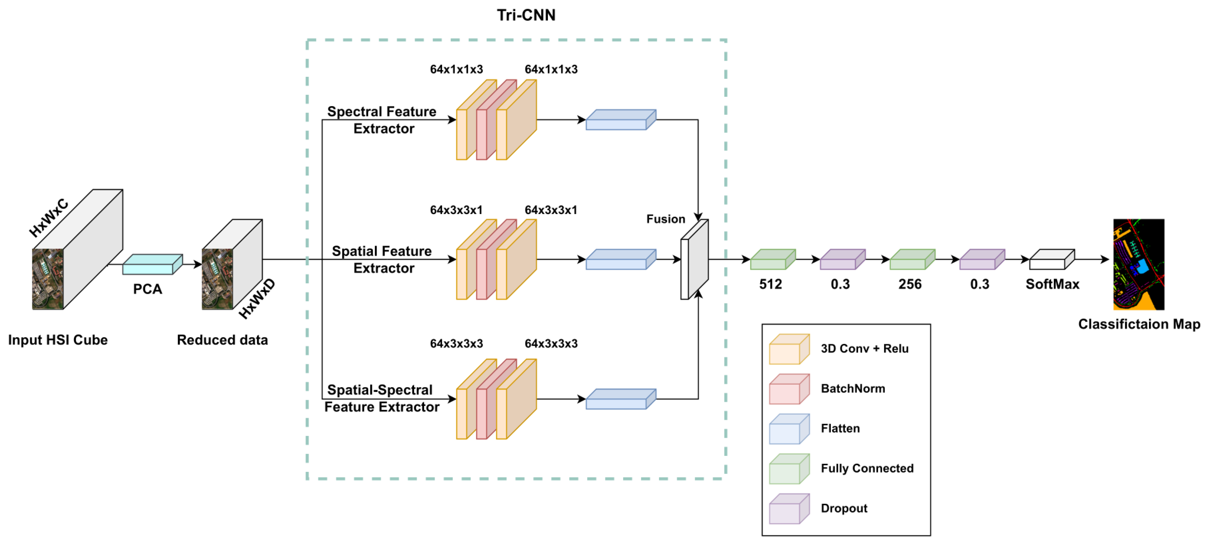
- A new model that incorporates feature extraction at different filter scales is proposed, which effectively improves the classification performance.
- A deep feature-learning network based on various dimensions with varied kernel sizes is created so that the filters may concurrently capture spectral, spatial, and spectral–spatial properties in order to more effectively use the spatial-spectral information in HSIs. The proposed model has a better ability to learn new features than other models that are already in use, according to experimental results.
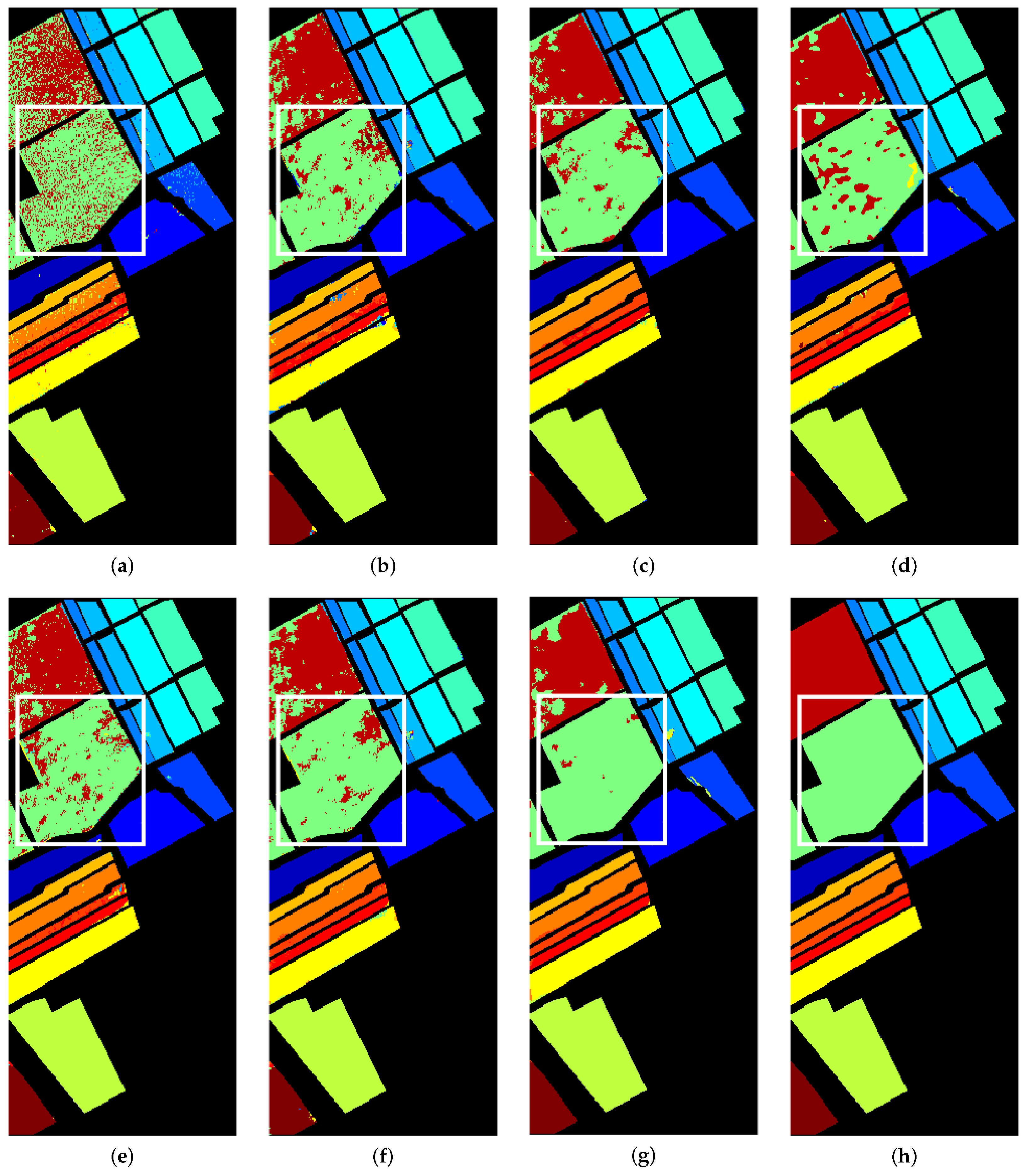
- The proposed model not only outperforms existing methods in the case of smaller number of samples, but also achieves better accuracy with enough training samples, according to statistical results from detailed trials on three HSIs that will be reported and discussed in the next sections.
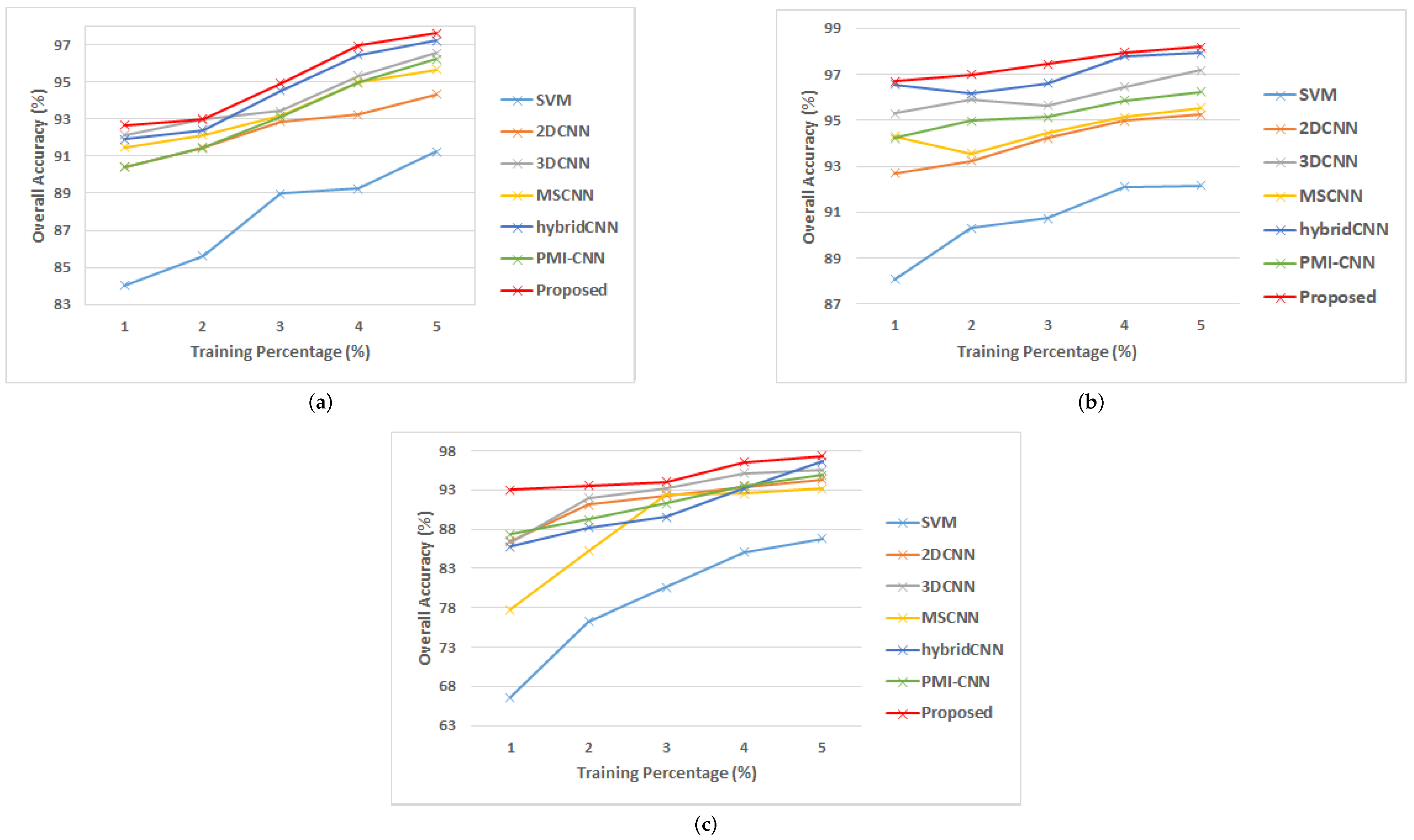
- The impact of different percentages of training data on model performance in terms of OA, AA and kappa metrics are also examined.
2. Methodology
2.1. Framework of the Proposed Model
2.1.1. Data Preprocessing
2.1.2. Architecture of the Proposed Tri-CNN
2.2. Loss Function
3. Experiments and Analysis
3.1. Datasets
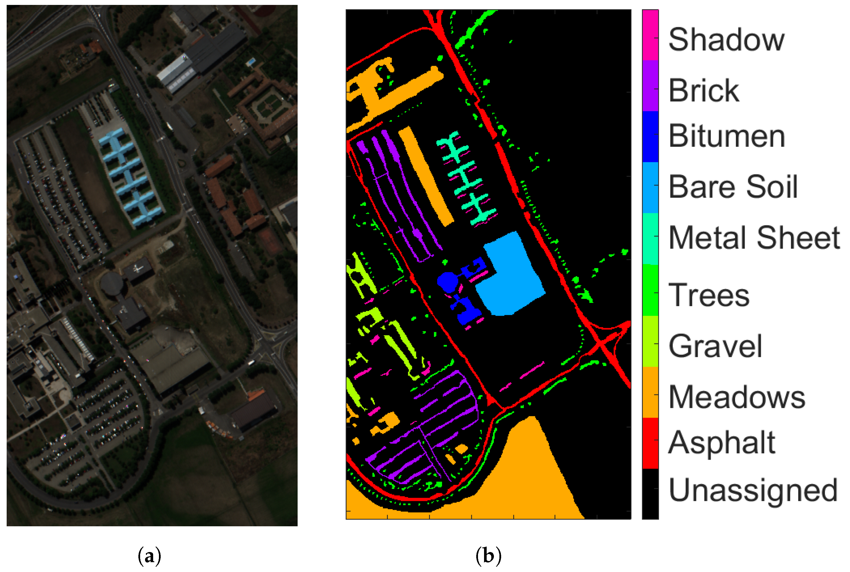
- Pavia University (PU): This is a scene acquired with the Reflective Optics Imaging Spectrometer Sensor (ROSIS) during a flight campaign over Pavia, northern Italy. The image consists of 103 spectral bands with wavelengths ranging from 0.43 to 0.86 m and a spatial resolution of 1.3 m. The size of Pavia University is pixels. Figure 2a shows RGB color composite of the scene. The reference classification map in Figure 2b shows nine classes, with the unassigned pixels colored in black and labeled as Unassigned. Table 1 shows the number of pixels per each class in the data set.
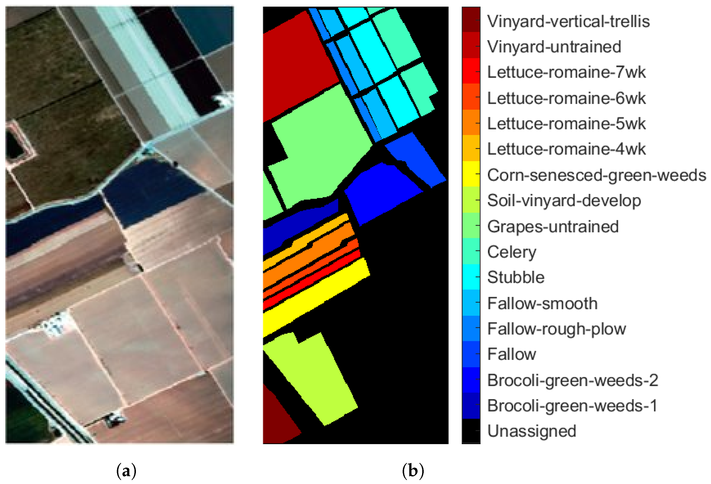
- Salinas (SA): This scene was collected by the Airborne Visible/Infrared Imaging Spectrometer (AVIRIS) sensor over Salinas Valley, California. The image consists of 224 spectral bands with wavelengths ranging from 0.4 to 2.45 m and a spatial resolution of 3.7 m. The size of Salinas is pixels. Bands 108–112, 154–167, and 224 were removed due to distortions from water absorption. Figure 3a shows RGB composite of the scene. The reference classification map in Figure 3b shows that Salinas ground truth class map contains 16 classes. Similar to PU, unassigned pixels are colored in black and labeled as Unassigned. Table 2 shows number of pixels per class in the data set.
- Mississippi Gulfport (GP): The dataset was collected over the University of Southern Mississippi’s-Gulfpark Campus [52]. The image consists of 72 bands with wavelengths ranging from 0.37 to 1.04 m and a spatial resolution of 1.0 m. The size of GP is pixels. Figure 4a shows RGB color composite of the scene. The reference classification map in Figure 4b shows six classes. As with PU and SA datasets, the unassigned pixels in the image are colored in black and labeled as Unassigned. Table 3 shows the number of pixels per class in the dataset.
3.2. Evaluation Metrics
3.3. Experimental Configuration
3.4. Experimental Results
3.4.1. Analysis of Parameters
3.4.2. Ablation Studies
3.4.3. Comparison with Other Methods
3.4.4. Performance of Different Models at Different Percentages of Training Data
4. Conclusions
Author Contributions
Funding
Data Availability Statement
Conflicts of Interest
References
- Moroni, M.; Lupo, E.; Marra, E.; Cenedese, A. Hyperspectral image analysis in environmental monitoring: Setup of a new tunable filter platform. Procedia Environ. Sci. 2013, 19, 885–894. [Google Scholar] [CrossRef] [Green Version]
- Stuart, M.B.; McGonigle, A.J.; Willmott, J.R. Hyperspectral imaging in environmental monitoring: A review of recent developments and technological advances in compact field deployable systems. Sensors 2019, 19, 3071. [Google Scholar] [CrossRef] [PubMed] [Green Version]
- Ad ao, T.; Hruška, J.; Pádua, L.; Bessa, J.; Peres, E.; Morais, R.; Sousa, J.J. Hyperspectral imaging: A review on UAV-based sensors, data processing and applications for agriculture and forestry. Remote Sens. 2017, 9, 1110. [Google Scholar] [CrossRef] [Green Version]
- Dale, L.M.; Thewis, A.; Boudry, C.; Rotar, I.; Dardenne, P.; Baeten, V.; Pierna, J.A.F. Hyperspectral imaging applications in agriculture and agro-food product quality and safety control: A review. Appl. Spectrosc. Rev. 2013, 48, 142–159. [Google Scholar] [CrossRef]
- Park, B.; Lu, R. Hyperspectral Imaging Technology in Food and Agriculture; Springer: Berlin/Heidelberg, Germany, 2015. [Google Scholar]
- Lu, B.; Dao, P.D.; Liu, J.; He, Y.; Shang, J. Recent advances of hyperspectral imaging technology and applications in agriculture. Remote Sens. 2020, 12, 2659. [Google Scholar] [CrossRef]
- Boubanga-Tombet, S.; Huot, A.; Vitins, I.; Heuberger, S.; Veuve, C.; Eisele, A.; Hewson, R.; Guyot, E.; Marcotte, F.; Chamberland, M. Thermal infrared hyperspectral imaging for mineralogy mapping of a mine face. Remote Sens. 2018, 10, 1518. [Google Scholar] [CrossRef] [Green Version]
- Kereszturi, G.; Schaefer, L.N.; Miller, C.; Mead, S. Hydrothermal alteration on composite volcanoes: Mineralogy, hyperspectral imaging, and aeromagnetic study of Mt Ruapehu, New Zealand. Geochem. Geophys. Geosystems 2020, 21, e2020GC009270. [Google Scholar] [CrossRef]
- Johnson, C.L.; Browning, D.A.; Pendock, N.E. Hyperspectral imaging applications to geometallurgy: Utilizing blast hole mineralogy to predict Au-Cu recovery and throughput at the Phoenix mine, Nevada. Econ. Geol. 2019, 114, 1481–1494. [Google Scholar] [CrossRef]
- Yuen, P.W.; Richardson, M. An introduction to hyperspectral imaging and its application for security, surveillance and target acquisition. Imaging Sci. J. 2010, 58, 241–253. [Google Scholar] [CrossRef]
- Stein, D.; Schoonmaker, J.; Coolbaugh, E. Hyperspectral Imaging for Intelligence, Surveillance, and Reconnaissance; Technical report; Space and Naval Warfare Systems Center: San Diego, CA, USA, 2001. [Google Scholar]
- Koz, A. Ground-Based Hyperspectral Image Surveillance Systems for Explosive Detection: Part I—State of the Art and Challenges. IEEE J. Sel. Top. Appl. Earth Obs. Remote Sens. 2019, 12, 4746–4753. [Google Scholar] [CrossRef]
- Ghamisi, P.; Yokoya, N.; Li, J.; Liao, W.; Liu, S.; Plaza, J.; Rasti, B.; Plaza, A. Advances in hyperspectral image and signal processing: A comprehensive overview of the state of the art. IEEE Geosci. Remote Sens. Mag. 2017, 5, 37–78. [Google Scholar] [CrossRef] [Green Version]
- Li, S.; Song, W.; Fang, L.; Chen, Y.; Ghamisi, P.; Benediktsson, J.A. Deep learning for hyperspectral image classification: An overview. IEEE Trans. Geosci. Remote Sens. 2019, 57, 6690–6709. [Google Scholar] [CrossRef] [Green Version]
- Bellman, R.E. Dynamic programming. Science 1966, 153, 34–37. [Google Scholar] [CrossRef]
- Melgani, F.; Bruzzone, L. Classification of hyperspectral remote sensing images with support vector machines. IEEE Trans. Geosci. Remote Sens. 2004, 42, 1778–1790. [Google Scholar] [CrossRef] [Green Version]
- Wang, X. Hyperspectral Image Classification Powered by Khatri-Rao Decomposition based Multinomial Logistic Regression. IEEE Trans. Geosci. Remote Sens. 2022, 60, 5530015. [Google Scholar] [CrossRef]
- Joelsson, S.R.; Benediktsson, J.A.; Sveinsson, J.R. Random forest classifiers for hyperspectral data. In Proceedings of the 2005 IEEE International Geoscience and Remote Sensing Symposium, IGARSS’05, Seoul, Republic of Korea, 25–29 July 2005; IEEE: Piscataway, NJ, USA, 2005; Volume 1, p. 4. [Google Scholar]
- Luo, K.; Qin, Y.; Yin, D.; Xiao, H. Hyperspectral image classification based on pre-post combination process. In Proceedings of the 2019 6th International Conference on Systems and Informatics (ICSAI), Shanghai, China, 2–4 November 2019; IEEE: Piscataway, NJ, USA, 2019; pp. 1275–1279. [Google Scholar]
- Windrim, L.; Ramakrishnan, R.; Melkumyan, A.; Murphy, R.J.; Chlingaryan, A. Unsupervised feature-learning for hyperspectral data with autoencoders. Remote Sens. 2019, 11, 864. [Google Scholar] [CrossRef] [Green Version]
- Li, Z.; Huang, H.; Zhang, Z.; Shi, G. Manifold-Based Multi-Deep Belief Network for Feature Extraction of Hyperspectral Image. Remote Sens. 2022, 14, 1484. [Google Scholar] [CrossRef]
- Zhu, L.; Chen, Y.; Ghamisi, P.; Benediktsson, J.A. Generative adversarial networks for hyperspectral image classification. IEEE Trans. Geosci. Remote Sens. 2018, 56, 5046–5063. [Google Scholar] [CrossRef]
- Bai, J.; Lu, J.; Xiao, Z.; Chen, Z.; Jiao, L. Generative adversarial networks based on transformer encoder and convolution block for hyperspectral image classification. Remote Sens. 2022, 14, 3426. [Google Scholar] [CrossRef]
- Mou, L.; Ghamisi, P.; Zhu, X. Deep Recurrent Neural Networks for Hyperspectral Image Classification. IEEE Trans. Geosci. Remote Sens. 2017, 55, 3639–3655. [Google Scholar] [CrossRef]
- Hang, R.; Liu, Q.; Hong, D.; Ghamisi, P. Cascaded recurrent neural networks for hyperspectral image classification. IEEE Trans. Geosci. Remote Sens. 2019, 57, 5384–5394. [Google Scholar] [CrossRef] [Green Version]
- Fukunaga, K. Introduction to Statistical Pattern Recognition; Elsevier: Amsterdam, The Netherlands, 2013. [Google Scholar]
- Zhou, M.; Samiappan, S.; Worch, E.; Ball, J.E. Hyperspectral Image Classification Using Fisher’s Linear Discriminant Analysis Feature Reduction with Gabor Filtering and CNN. In Proceedings of the IGARSS 2020-2020 IEEE International Geoscience and Remote Sensing Symposium, Waikoloa, HI, USA, 26 September–2 October 2020; IEEE: Piscataway, NJ, USA, 2020; pp. 493–496. [Google Scholar]
- Ali, U.M.E.; Hossain, M.A.; Islam, M.R. Analysis of PCA based feature extraction methods for classification of hyperspectral image. In Proceedings of the 2019 2nd International Conference on Innovation in Engineering and Technology (ICIET), Dhaka, Bangladesh, 23–24 December 2019; IEEE: Piscataway, NJ, USA, 2019; pp. 1–6. [Google Scholar]
- Sun, Q.; Liu, X.; Fu, M. Classification of hyperspectral image based on principal component analysis and deep learning. In Proceedings of the 2017 7th IEEE International Conference on Electronics Information and Emergency Communication (ICEIEC), Shenzhen, China, 21–23 July 2017; IEEE: Piscataway, NJ, USA, 2017; pp. 356–359. [Google Scholar]
- Fauvel, M.; Chanussot, J.; Benediktsson, J.A. Kernel principal component analysis for the classification of hyperspectral remote sensing data over urban areas. EURASIP J. Adv. Signal Process. 2009, 2009, 1–14. [Google Scholar] [CrossRef] [Green Version]
- Ruiz, D.; Bacca, B.; Caicedo, E. Hyperspectral images classification based on inception network and kernel PCA. IEEE Lat. Am. Trans. 2019, 17, 1995–2004. [Google Scholar] [CrossRef]
- Paoletti, M.; Haut, J.; Plaza, J.; Plaza, A. A new deep convolutional neural network for fast hyperspectral image classification. ISPRS J. Photogramm. Remote Sens. 2018, 145, 120–147. [Google Scholar] [CrossRef]
- Tun, N.L.; Gavrilov, A.; Tun, N.M.; Trieu, D.M.; Aung, H. Hyperspectral Remote Sensing Images Classification Using Fully Convolutional Neural Network. In Proceedings of the IEEE Conference of Russian Young Researchers in Electrical and Electronic Engineering (ElConRus), St. Petersburg, Russia, 26–29 January 2021; pp. 2166–2170. [Google Scholar] [CrossRef]
- Lin, L.; Chen, C.; Xu, T. Spatial-spectral hyperspectral image classification based on information measurement and CNN. EURASIP J. Wirel. Commun. Netw. 2020, 2020, 1–16. [Google Scholar] [CrossRef]
- Li, X.; Ding, M.; Pižurica, A. Deep Feature Fusion via Two-Stream Convolutional Neural Network for Hyperspectral Image Classification. IEEE Trans. Geosci. Remote Sens. 2020, 58, 2615–2629. [Google Scholar] [CrossRef] [Green Version]
- Kanthi, M.; Sarma, T.H.; Bindu, C.S. A 3d-Deep CNN Based Feature Extraction and Hyperspectral Image Classification. In Proceedings of the 2020 IEEE India Geoscience and Remote Sensing Symposium (InGARSS), Online, 1–4 December 2020; IEEE: Piscataway, NJ, USA, 2020; pp. 229–232. [Google Scholar]
- Ahmad, M.; Khan, A.M.; Mazzara, M.; Distefano, S.; Ali, M.; Sarfraz, M.S. A fast and compact 3-D CNN for hyperspectral image classification. IEEE Geosci. Remote Sens. Lett. 2020, 19, 5502205. [Google Scholar] [CrossRef]
- Chang, Y.L.; Tan, T.H.; Lee, W.H.; Chang, L.; Chen, Y.N.; Fan, K.C.; Alkhaleefah, M. Consolidated Convolutional Neural Network for Hyperspectral Image Classification. Remote Sens. 2022, 14, 1571. [Google Scholar] [CrossRef]
- Sun, K.; Wang, A.; Sun, X.; Zhang, T. Hyperspectral image classification method based on M-3DCNN-Attention. J. Appl. Remote Sens. 2022, 16, 026507. [Google Scholar] [CrossRef]
- Li, W.; Chen, H.; Liu, Q.; Liu, H.; Wang, Y.; Gui, G. Attention Mechanism and Depthwise Separable Convolution Aided 3DCNN for Hyperspectral Remote Sensing Image Classification. Remote Sens. 2022, 14, 2215. [Google Scholar] [CrossRef]
- Yang, X.; Zhang, X.; Ye, Y.; Lau, R.Y.; Lu, S.; Li, X.; Huang, X. Synergistic 2D/3D convolutional neural network for hyperspectral image classification. Remote Sens. 2020, 12, 2033. [Google Scholar] [CrossRef]
- Roy, S.K.; Krishna, G.; Dubey, S.R.; Chaudhuri, B.B. HybridSN: Exploring 3-D–2-D CNN Feature Hierarchy for Hyperspectral Image Classification. IEEE Geosci. Remote Sens. Lett. 2020, 17, 277–281. [Google Scholar] [CrossRef] [Green Version]
- Guo, H.; Liu, J.; Yang, J.; Xiao, Z.; Wu, Z. Deep Collaborative Attention Network for Hyperspectral Image Classification by Combining 2-D CNN and 3-D CNN. IEEE J. Sel. Top. Appl. Earth Obs. Remote Sens. 2021, 13, 4789–4802. [Google Scholar] [CrossRef]
- Ghaderizadeh, S.; Abbasi-Moghadam, D.; Sharifi, A.; Zhao, N.; Tariq, A. Hyperspectral Image Classification Using a Hybrid 3D-2D Convolutional Neural Networks. IEEE J. Sel. Top. Appl. Earth Obs. Remote Sens. 2021, 14, 7570–7588. [Google Scholar] [CrossRef]
- Zhang, H.; Li, Y.; Jiang, Y.; Wang, P.; Shen, Q.; Shen, C. Hyperspectral classification based on lightweight 3-D-CNN with transfer learning. IEEE Trans. Geosci. Remote Sens. 2019, 57, 5813–5828. [Google Scholar] [CrossRef] [Green Version]
- Xu, Y.; Du, B.; Zhang, L. Robust self-ensembling network for hyperspectral image classification. IEEE Trans. Neural Netw. Learn. Syst. 2022, 1–14. [Google Scholar] [CrossRef]
- Yu, H.; Xu, Z.; Zheng, K.; Hong, D.; Yang, H.; Song, M. MSTNet: A Multilevel Spectral–Spatial Transformer Network for Hyperspectral Image Classification. IEEE Trans. Geosci. Remote Sens. 2022, 60, 1–13. [Google Scholar] [CrossRef]
- Wu, S.; Zhang, J.; Zhong, C. Multiscale spectral–spatial unified networks for hyperspectral image classification. In Proceedings of the IGARSS 2019-2019 IEEE International Geoscience and Remote Sensing Symposium, Yokohama, Japan, 28 July–2 August 2019; IEEE: Piscataway, NJ, USA, 2019; pp. 2706–2709. [Google Scholar]
- Xu, Y.; Zhang, L.; Du, B.; Zhang, F. Spectral–spatial unified networks for hyperspectral image classification. IEEE Trans. Geosci. Remote Sens. 2018, 56, 5893–5909. [Google Scholar] [CrossRef]
- Zhong, H.; Li, L.; Ren, J.; Wu, W.; Wang, R. Hyperspectral image classification via parallel multi-input mechanism-based convolutional neural network. Multimed. Tools Appl. 2022, 1–26. [Google Scholar] [CrossRef]
- Pei, S.; Song, H.; Lu, Y. Small Sample Hyperspectral Image Classification Method Based on Dual-Channel Spectral Enhancement Network. Electronics 2022, 11, 2540. [Google Scholar] [CrossRef]
- Gader, P.; Zare, A.; Close, R.; Aitken, J.; Tuell, G. Muufl Gulfport Hyperspectral and Lidar Airborne Data Set; Technical Report REP-2013-570; University Florida: Gainesville, FL, USA, 2013. [Google Scholar]
- Nyasaka, D.; Wang, J.; Tinega, H. Learning hyperspectral feature extraction and classification with resnext network. arXiv 2020, arXiv:2002.02585. [Google Scholar]
- Song, H.; Yang, W.; Dai, S.; Yuan, H. Multi-source remote sensing image classification based on two-channel densely connected convolutional networks. Math. Biosci. Eng. 2020, 17, 7353–7378. [Google Scholar] [CrossRef] [PubMed]
- Chen, Y.; Jiang, H.; Li, C.; Jia, X.; Ghamisi, P. Deep feature extraction and classification of hyperspectral images based on convolutional neural networks. IEEE Trans. Geosci. Remote Sens. 2016, 54, 6232–6251. [Google Scholar] [CrossRef] [Green Version]
- Hamida, A.B.; Benoit, A.; Lambert, P.; Amar, C.B. 3-D deep learning approach for remote sensing image classification. IEEE Trans. Geosci. Remote Sens. 2018, 56, 4420–4434. [Google Scholar] [CrossRef]




| Class | Name | Total Samples |
|---|---|---|
| 1 | Asphalt | 6631 |
| 2 | Meadows | 18,649 |
| 3 | Gravel | 2099 |
| 4 | Trees | 3064 |
| 5 | Painted Metal Sheet | 1345 |
| 6 | Bare Soil | 5029 |
| 7 | Bitumen | 1330 |
| 8 | Self-Blocking Bricks | 3682 |
| 9 | Shadows | 947 |
| Total | 42,776 |
| Class | Name | Total Samples |
|---|---|---|
| 1 | Brocoli-green-weeds-1 | 2009 |
| 2 | Brocoli-green-weeds-2 | 3726 |
| 3 | Fallow | 1976 |
| 4 | Fallow-rough-plow | 1394 |
| 5 | Fallow-smooth | 2678 |
| 6 | Stubble | 3959 |
| 7 | Celery | 3579 |
| 8 | Grapes-untrained | 11,271 |
| 9 | Soil-vinyard-develop | 6203 |
| 10 | Corn-senesced-green-weeds | 3278 |
| 11 | Lettuce-romaine-4wk | 1068 |
| 12 | Lettuce-romaine-5wk | 1927 |
| 13 | Lettuce-romaine-6wk | 916 |
| 14 | Lettuce-romaine-7wk | 1070 |
| 15 | Vinyard-untrained | 7268 |
| 16 | Vinyard-vertical-trellis | 1807 |
| Total | 54,129 |
| Class | Name | Total Samples |
|---|---|---|
| 1 | Dirt | 175 |
| 2 | Asphalt | 1657 |
| 3 | Dead Grass | 438 |
| 4 | Grass | 970 |
| 5 | Shadow | 527 |
| 6 | Trees | 2330 |
| Total | 6097 |
| Proposed Model Configuration | ||
|---|---|---|
| Spectral Feature Learning | Spatial Feature Learning | Spectral–Spatial Feature Learning |
| Input:(13 × 13 × 15 × 1) | ||
| 3DConv-(1,1,3,64), stride = 1, padding = 0 | 3DConv-(3,3,1,64), stride = 1, padding = 0 | 3DConv-(3,3,3,64), stride = 1, padding = 0 |
| Output10:(13 × 13 × 13 × 64) | Output20:(11 × 11 × 15 × 64) | Output30:(11 × 11 × 13 × 64) |
| 3DConv-(1,1,3,64), stride = 1, padding = 0 | 3DConv-(3,3,1,64), stride = 1, padding = 0 | 3DConv-(3,3,3,64), stride = 1, padding = 0 |
| Output11:(13 × 13 × 11 × 64) | Output21:(9 × 9 × 15 × 64) | Output31:(9 × 9 × 11 × 64) |
| Flatten | Flatten | Flatten |
| Output12:(118,976) | Output22:(77,760) | Output32:(57,024) |
| Concat(Output12,Output22,Output32) | ||
| FC-(253,760,512) | ||
| Dropout(0.3) | ||
| FC-(512,256) | ||
| Dropout(0.3) | ||
| FC-(256,9) | ||
| Output:(9) | ||
| Dataset | Window Size | Spectral Dimension |
|---|---|---|
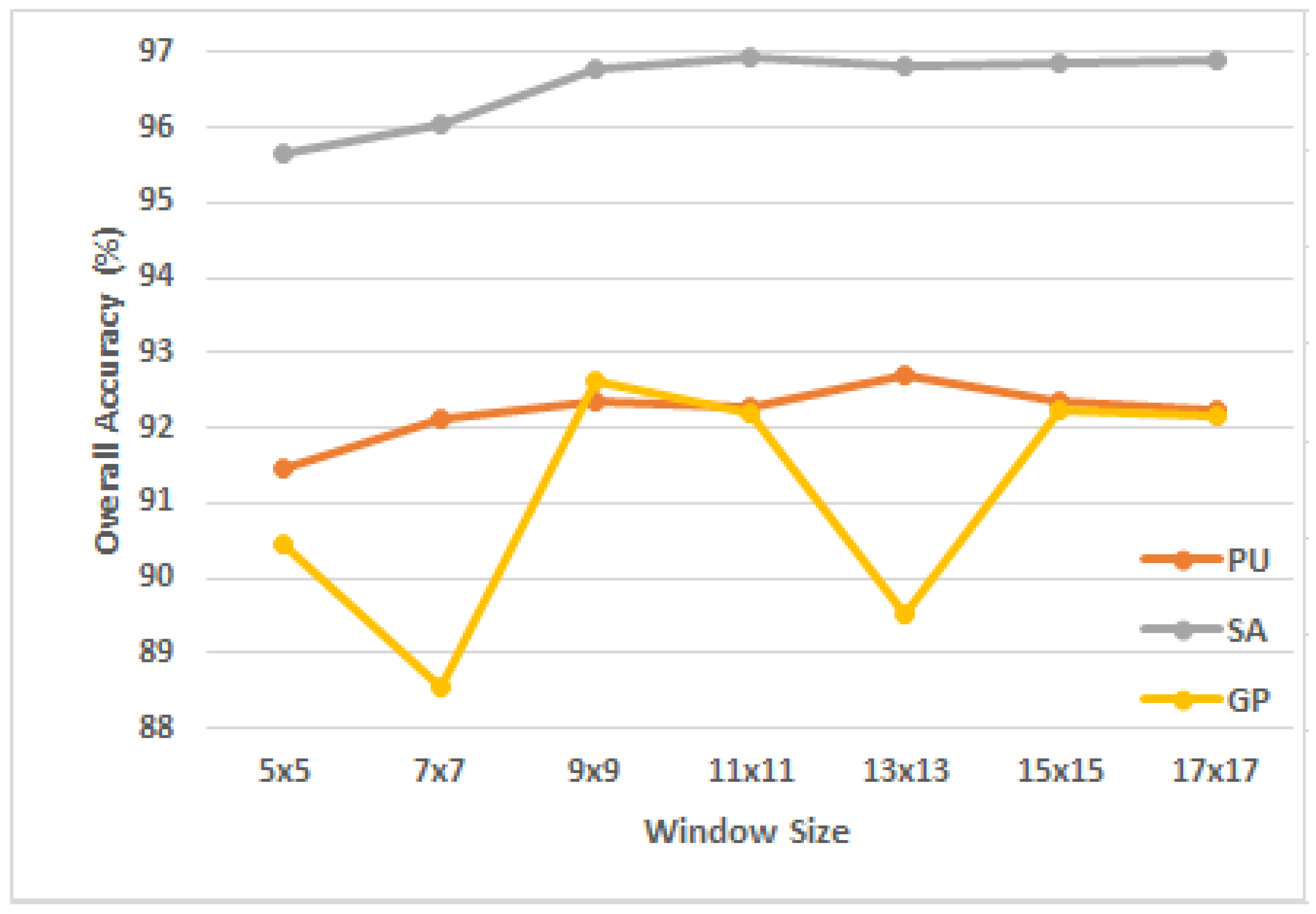
| PU | 15 | |
| SA | 35 | |
| GP | 45 |
| Method | Spectral Only | Spatial Only | Spectral–Spatial Only | Spectral + Spatial | Spectral + Spectral–Spatial | Spatial + Spectral–Spatial | Proposed |
|---|---|---|---|---|---|---|---|
| Overall Accuracy (%) | 85.63 ± 4.42 | 89.45 ± 2.58 | 91.43 ± 1.93 | 90.88 ± 3.74 | 91.41 ± 1.57 | 91.51 ± 2.18 | 92.96 ± 1.05 |
| Average Accuracy (%) | 82.44 ± 3.28 | 85.21 ± 3.30 | 88.23 ± 2.32 | 87.70 ± 2.55 | 88.67 ± 2.84 | 89.48 ± 3.90 | 89.53 ± 1.39 |
| Kappa | 79.31 ± 4.28 | 87.90 ± 2.40 | 89.26 ± 2.43 | 88.89 ± 3.74 | 90.06 ± 1.13 | 90.16 ± 1.23 | 90.56 ± 2.53 |
| Class | Train | Test | SVM | 2DCNN | 3DCNN | PMI-CNN | HybridSN | MSCNN | Proposed |
|---|---|---|---|---|---|---|---|---|---|
| 1 | 66 | 6565 | 83.59 | 92.91 | 94.7821 | 99.17 | 94.48 | 91.96 | 81.01 |
| 2 | 186 | 18,463 | 88.88 | 98.83 | 99.10 | 99.31 | 99.66 | 99.22 | 97.04 |
| 3 | 21 | 2078 | 63.22 | 76.22 | 71.89 | 77.37 | 77.46 | 70.98 | 86.08 |
| 4 | 31 | 3033 | 85.73 | 85.08 | 87.46 | 76.72 | 83.25 | 82.99 | 85.47 |
| 5 | 13 | 1332 | 99.40 | 99.85 | 99.33 | 99.22 | 99.85 | 98.51 | 99.43 |
| 6 | 50 | 4979 | 79.39 | 76.21 | 78.38 | 89.93 | 89.73 | 84.19 | 99.32 |
| 7 | 13 | 1317 | 61.42 | 79.69 | 90.30 | 59.47 | 90.00 | 74.66 | 73.30 |
| 8 | 37 | 3645 | 75.58 | 77.59 | 83.70 | 55.48 | 74.47 | 85.95 | 95.00 |
| 9 | 10 | 937 | 99.23 | 83.10 | 94.19 | 94.82 | 91.34 | 82.36 | 99.36 |
| Overall Accuracy (%) | 84.03 ± 3.33 | 90.42 ± 4.80 | 92.13 ± 2.19 | 90.40 ± 2.42 | 92.34 ± 2.74 | 91.48 ± 2.07 | 92.66 ± 2.24 | ||
| Average Accuracy (%) | 81.89 ± 4.41 | 85.50 ± 2.50 | 88.29 ± 2.41 | 83.59 ± 4.82 | 88.80 ± 2.86 | 85.65 ± 3.16 | 90.65 ± 2.37 | ||
| Kappa × 100 | 78.98 ± 3.44 | 87.13 ± 2.35 | 89.44 ± 1.25 | 87.14 ± 2.57 | 89.17 ± 1.59 | 88.57 ± 1.09 | 90.31 ± 1.31 | ||
| Class | Train | Test | SVM | 2DCNN | 3DCNN | PMI-CNN | HybridSN | MSCNN | Proposed |
|---|---|---|---|---|---|---|---|---|---|
| 1 | 20 | 1989 | 98.65 | 99.75 | 100.00 | 98.35 | 100.00 | 99.15 | 100.00 |
| 2 | 37 | 3689 | 99.38 | 100.00 | 100.00 | 100.00 | 99.91 | 99.94 | 100.00 |
| 3 | 20 | 1956 | 93.01 | 99.69 | 100.00 | 99.54 | 98.48 | 99.94 | 97.72 |
| 4 | 14 | 1380 | 96.05 | 98.63 | 99.56 | 99.13 | 98.85 | 95.33 | 96.05 |
| 5 | 27 | 2651 | 97.16 | 96.19 | 99.25 | 98.80 | 100.00 | 97.49 | 97.16 |
| 6 | 39 | 3920 | 99.36 | 99.57 | 100.00 | 100.00 | 99.92 | 99.94 | 99.44 |
| 7 | 36 | 3543 | 99.05 | 99.18 | 99.77 | 99.87 | 99.63 | 99.69 | 99.94 |
| 8 | 113 | 11,158 | 80.03 | 87.88 | 90.61 | 85.67 | 88.20 | 90.95 | 98.65 |
| 9 | 62 | 6141 | 99.41 | 99.98 | 99.88 | 100.00 | 99.90 | 100.00 | 100.00 |
| 10 | 33 | 3245 | 95.79 | 96.27 | 97.52 | 99.20 | 96.70 | 96.36 | 98.16 |
| 11 | 11 | 1057 | 95.22 | 95.31 | 99.15 | 98.22 | 96.25 | 98.40 | 99.53 |
| 12 | 19 | 1908 | 88.16 | 95.53 | 97.40 | 99.74 | 96.26 | 98.33 | 95.95 |
| 13 | 9 | 907 | 64.19 | 63.75 | 79.58 | 79.47 | 61.68 | 96.83 | 99.78 |
| 14 | 11 | 1059 | 89.81 | 86.16 | 97.28 | 96.54 | 98.13 | 97.19 | 98.41 |
| 15 | 72 | 7196 | 60.29 | 77.43 | 85.23 | 84.35 | 90.54 | 77.49 | 82.42 |
| 16 | 18 | 1789 | 97.45 | 97.95 | 99.16 | 99.28 | 99.05 | 97.67 | 99.88 |
| Overall Accuracy (%) | 88.08 ± 2.56 | 92.68 ± 1.69 | 95.30 ± 1.43 | 94.22 ± 2.85 | 95.54 ± 1.12 | 94.29± 2.23 | 96.68 ± 2.11 | ||
| Average Accuracy (%) | 90.81 ± 2.11 | 93.33 ± 2.77 | 96.52 ± 9.26 | 96.14 ± 1.47 | 95.31 ± 1.17 | 96.54 ± 1.14 | 97.69 ± 1.09 | ||
| Kappa × 100 | 86.70 ± 1.10 | 91.85 ± 1.10 | 94.76 ± 1.59 | 93.57 ± 2.95 | 94.49 ± 1.24 | 93.63 ± 2.23 | 96.30 ± 2.10 | ||
| Class | Train | Test | SVM | 2DCNN | 3DCNN | PMI-CNN | HybridSN | MSCNN | Proposed |
|---|---|---|---|---|---|---|---|---|---|
| 1 | 2 | 173 | 1.71 | 2.28 | 16.00 | 3.42 | 13.42 | 2.28 | 86.85 |
| 2 | 16 | 1641 | 84.12 | 96.25 | 98.61 | 99.63 | 92.43 | 84.73 | 99.69 |
| 3 | 4 | 434 | 1.14 | 26.48 | 10.04 | 12.10 | 46.74 | 5.47 | 86.98 |
| 4 | 10 | 960 | 29.38 | 91.34 | 99.27 | 99.07 | 93.37 | 86.59 | 81.64 |
| 5 | 5 | 522 | 13.47 | 94.87 | 76.47 | 79.50 | 67.46 | 49.33 | 85.95 |
| 6 | 23 | 2307 | 98.71 | 93.13 | 94.03 | 95.83 | 97.95 | 94.72 | 96.05 |
| Overall Accuracy (%) | 66.55 ± 3.39 | 86.45 ± 1.29 | 86.32 ± 3.32 | 87.30 ± 4.95 | 87.79 ± 2.48 | 77.72 ± 3.28 | 92.96 ± 1.39 | ||
| Average Accuracy (%) | 38.09 ± 2.13 | 67.39 ± 3.57 | 65.74 ± 4.92 | 64.93 ± 3.72 | 69.06 ± 1.59 | 53.85 ± 2.73 | 89.53 ± 2.58 | ||
| Kappa × 100 | 49.44 ± 3.53 | 81.56 ± 2.42 | 81.24 ± 3.41 | 82.58 ± 4.29 | 82.41 ± 2.69 | 68.69 ± 3.44 | 90.56 ± 1.53 | ||
Disclaimer/Publisher’s Note: The statements, opinions and data contained in all publications are solely those of the individual author(s) and contributor(s) and not of MDPI and/or the editor(s). MDPI and/or the editor(s) disclaim responsibility for any injury to people or property resulting from any ideas, methods, instructions or products referred to in the content. |
© 2023 by the authors. Licensee MDPI, Basel, Switzerland. This article is an open access article distributed under the terms and conditions of the Creative Commons Attribution (CC BY) license (https://creativecommons.org/licenses/by/4.0/).
Share and Cite
Alkhatib, M.Q.; Al-Saad, M.; Aburaed, N.; Almansoori, S.; Zabalza, J.; Marshall, S.; Al-Ahmad, H. Tri-CNN: A Three Branch Model for Hyperspectral Image Classification. Remote Sens. 2023, 15, 316. https://doi.org/10.3390/rs15020316
Alkhatib MQ, Al-Saad M, Aburaed N, Almansoori S, Zabalza J, Marshall S, Al-Ahmad H. Tri-CNN: A Three Branch Model for Hyperspectral Image Classification. Remote Sensing. 2023; 15(2):316. https://doi.org/10.3390/rs15020316
Chicago/Turabian StyleAlkhatib, Mohammed Q., Mina Al-Saad, Nour Aburaed, Saeed Almansoori, Jaime Zabalza, Stephen Marshall, and Hussain Al-Ahmad. 2023. "Tri-CNN: A Three Branch Model for Hyperspectral Image Classification" Remote Sensing 15, no. 2: 316. https://doi.org/10.3390/rs15020316
APA StyleAlkhatib, M. Q., Al-Saad, M., Aburaed, N., Almansoori, S., Zabalza, J., Marshall, S., & Al-Ahmad, H. (2023). Tri-CNN: A Three Branch Model for Hyperspectral Image Classification. Remote Sensing, 15(2), 316. https://doi.org/10.3390/rs15020316


