2.1. EGMS Data
The key elements of the European Ground Motion Service (EGMS) are stated in the White Paper, available online at
https://land.copernicus.eu/user-corner/technical-library/egms-white-paper, accessed on 14 June 2022 [
37]. The purpose of the EGMS is to provide consistent, updated, standardized, harmonized information regarding ground deformation, all over Europe, to detect ground motion phenomena of any origin, natural or human-caused. The service is free and open, and the data will be updated on an annual basis. EGMS is included in the Copernicus Land Monitoring Service (CLSM,
https://www.copernicus.eu/en/copernicus-services/land, accessed on 14 June 2022 [
38]) and is based on the processing of ascending (ASC) and descending (DES) Sentinel-1 images (having pixel footprint 14 by 4 m), using full resolution Advanced SAR Interferometry (A-DInSAR) [
39]. This is complementary to Global Navigation Satellite Systems (GNSS) and other in situ observations. The EGMS includes archive images that in the case studies considered in this work start in 7 March 2015 and 17 June 2015, respectively for the ASC and DES orbits, and end the 31 December 2020. The acquisition revisit time is six days, which has been degraded to twelve days starting from December 2021, due to a failure of the Sentinel-1B satellite.
The EGMS includes three levels of products. The first level is the “basic” one, constituted by geocoded line of sight (LoS) deformation velocity maps, in ASC and DES orbits, where the measures are referred to a local reference point. The second level is the “calibrated” one, constituted by the product of the first level, mosaicked and integrated with Global Navigation Satellite Systems (GNSS) data. The second level measures do not refer to a local reference point. The third level is the “Ortho” one, constituted by deformation components along the vertical and east–west (E-W) directions, resampled to a grid with a cell size of 100 m. Useful information regarding the A-DInSAR approaches used in the EGMS is provided by Ferretti et al. (2021) [
40].
The 3D geolocation accuracy of the EGMS products is lower than 10 m [
41].
2.2. ADAfinder Tool
The ADAfinder tool is one of the four modules, called ADAtools [
35,
36], developed at the Research Unit of Geomatics of the Centre Tecnològic de Telecomunicacions de Catalunya (CTTC). The aim of the ADAtools is the semi-automatic extraction and preliminary analysis of ADA starting from the PSI-derived deformation maps. In particular, the ADAfinder tool has the main objective of identifying the ADA in the area of interest, starting from a dataset of persistent scatterers (PSs). An application that highlights its potential can be found in Tomás et al. [
42].
For a detailed description of the tools, see the user guide. In synthesis, the input is a file containing the dataset of PSs, in ESRI shapefile or .csv format. The main information necessary for each PSs is its coordinates, its mean deformation velocity (expressed in mm/year), and its deformation time series in the period of interest.
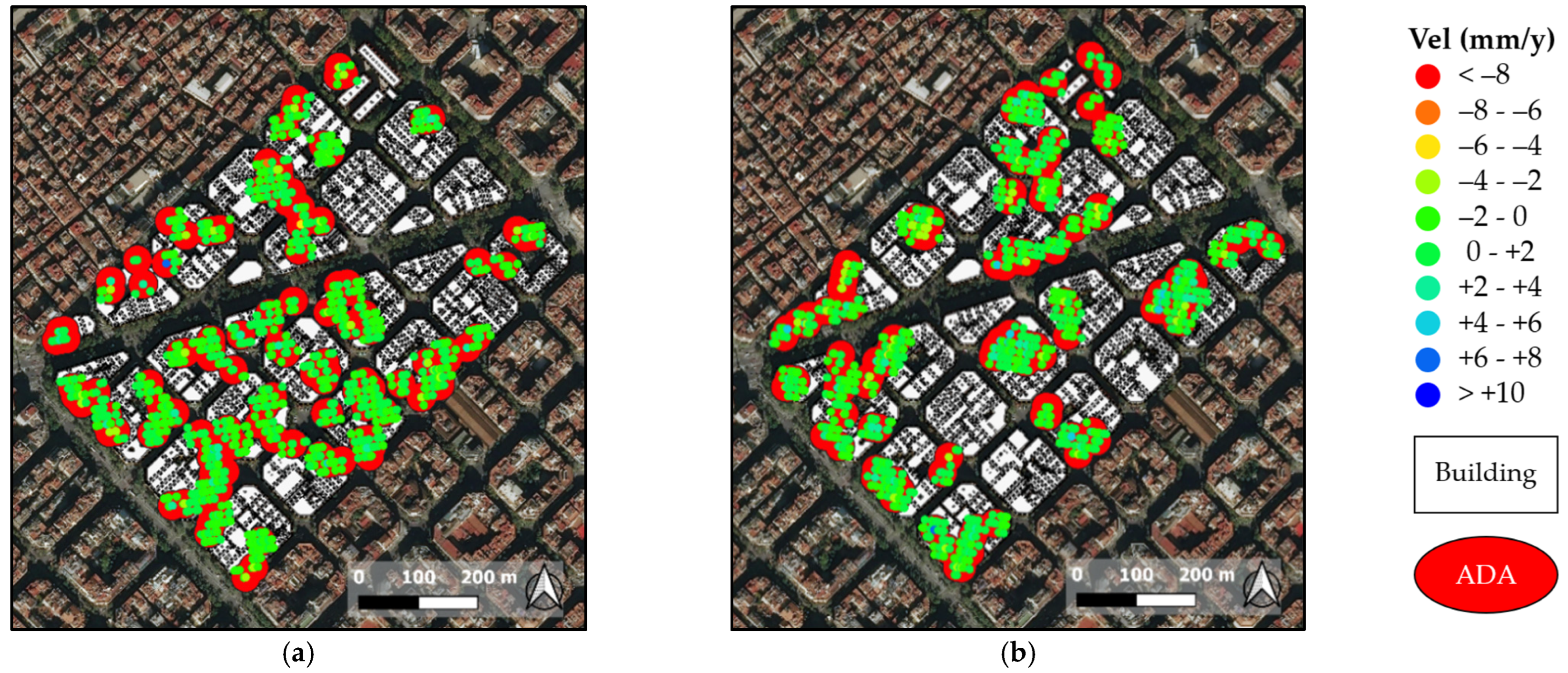
Initially, the “isolated” PSs and the “stable” PSs are removed. The first ones are defined as points with no other PSs around included within a defined distance, while the second ones are those PSs with a mean deformation velocity lower than a fixed “stability threshold”, in function of the standard deviation (σ) of the velocities of all the PSs of the dataset (Vm). Then, the clusters of PSs are detected and, finally, the ADA are identified on the basis of a radius of influence and of the minimum number of PSs set by the user.
The output of the ADAfinder tool consists of two ESRI shapefiles: one containing the polygons representing the ADA’s areas, and one containing the PSs included in the ADA. The statistics of the mean deformation velocity of each ADA are also provided.
It is important to underline that the lack of ADA could be related not only to the absence of an active deformation, but also to the absence of PSs [
43].
2.3. Proposed Methodology
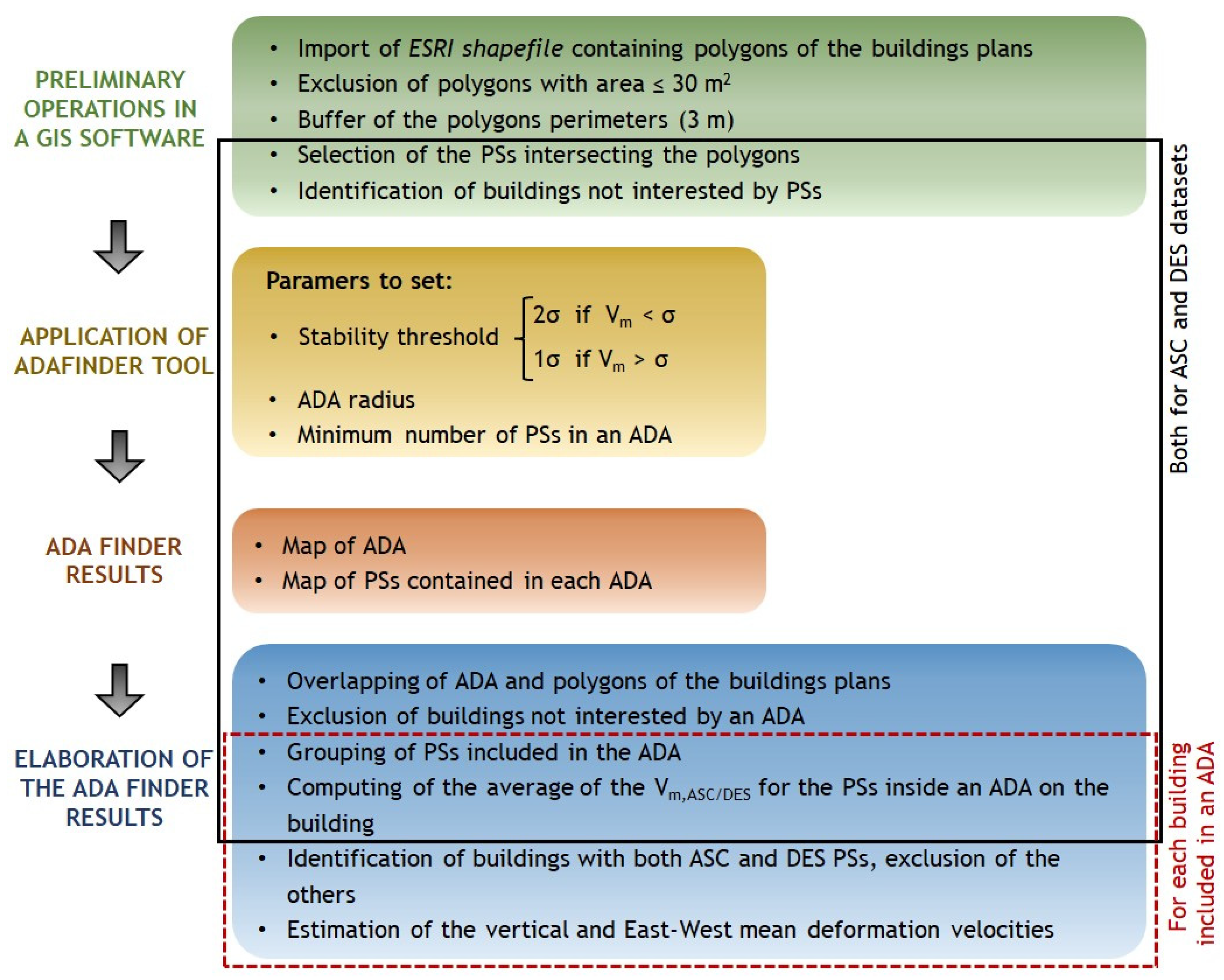
The proposed methodology is focused on finding buildings interested by deformations above an established threshold, in urbanized areas characterized by large dataset of PSs, through ADAfinder tool. The latter is included in a procedure that, for the first time, is specific for urban districts or whole municipalities/towns. A flowchart of the proposed methodology is shown in
Figure 1. The necessary data to implement the procedure are: (i) an
ESRI shapefile containing the polygons of the buildings plans and (ii) the two datasets referred to ASC and DES orbits, containing information about the PSs of the monitored area.
Since the proposed methodology is dedicated to data processing for SHM purposes, the introduction in the flowchart of preliminary operations to be performed in a GIS software, listed in the green box of the flowchart, is needed. The preliminary operations are aimed to PSs datasets filtering to direct the procedure towards the analysis of ADAs on the buildings. First, the ESRI shapefile containing polygons of the buildings plans is imported. The polygons with an area lower than 30 m2 are excluded, since they are not considered to be buildings. In fact, sometimes, other little elements can be included in the available shapefiles, for example cabins, canopies, small buildings, silos, or containers in harbor areas. Then, a buffer of the polygons perimeters is done in order to take into account the inaccuracies that they might have. Since the presented methodology is focused on the buildings, all the PSs related to any other construction or reflective target have to be discarded. For this reason, a selection of the PSs intersecting the polygons (including the buffer previously mentioned) is done, while the buildings not intersected by PSs are identified and pointed out. In future, a minimum number of points, such as their distribution on the building plan, could also be added as preliminary filter of the procedure, to exclude from the analysis the buildings not well represented.
Then, all the operations included in the black contour in
Figure 1 are separately done using both the ASC and DES datasets.
The following step is the application of the ADAfinder tool (yellow box of the flowchart). A criterion to establish the value of the stability threshold is to compare the V
m of the dataset of PSs with the relative σ. The original source of this criterion is to assume the stability threshold at 2σ to exclude all the points with lower V
m, as described in Barra et al. [
35]. Herein, a more conservative additional constraint is assumed, since the final goal is the identification of the critical constructions. In fact, the stability threshold is set at (i) 2σ if V
m < σ, while it is set at (ii) 1σ if V
m > σ. In general, if a high average value of the velocity is present (ii), it can be important to consider more constructions in the monitoring phase and then a lower threshold value can be fixed. In fact, in the case (i), the values of V
m are greater, and a trend of deformations more or less defined is present, so it is convenient to keep a larger number of PSs. In contrast, the case (i) usually verifies in large areas with different deformation processes included, so a great dispersion of the V
m values can be detected and a cut at 2σ is more convenient to exclude the lower deformation values.
Moreover, the ADA radius (in meters) should be set, and the minimum number of PSs in an ADA has to be imposed. In the proposed methodology, it is recommended to set the minimum number of PSs equal to the minimum value accepted by the tool, that, in the current version (ADAtools 2.0.3), is 3. The operation described until this step must be carried out both for the ASC and the DES datasets.
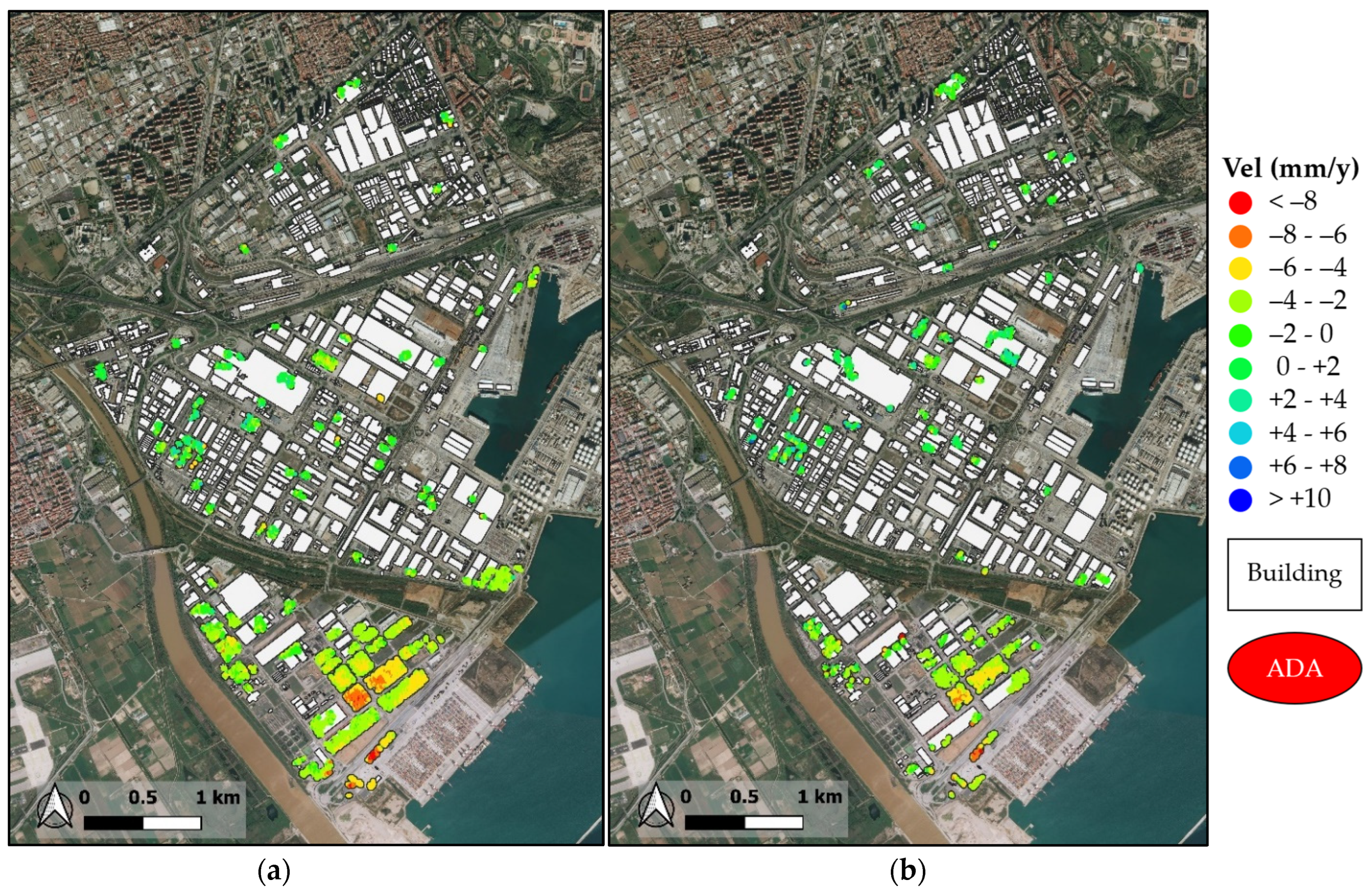
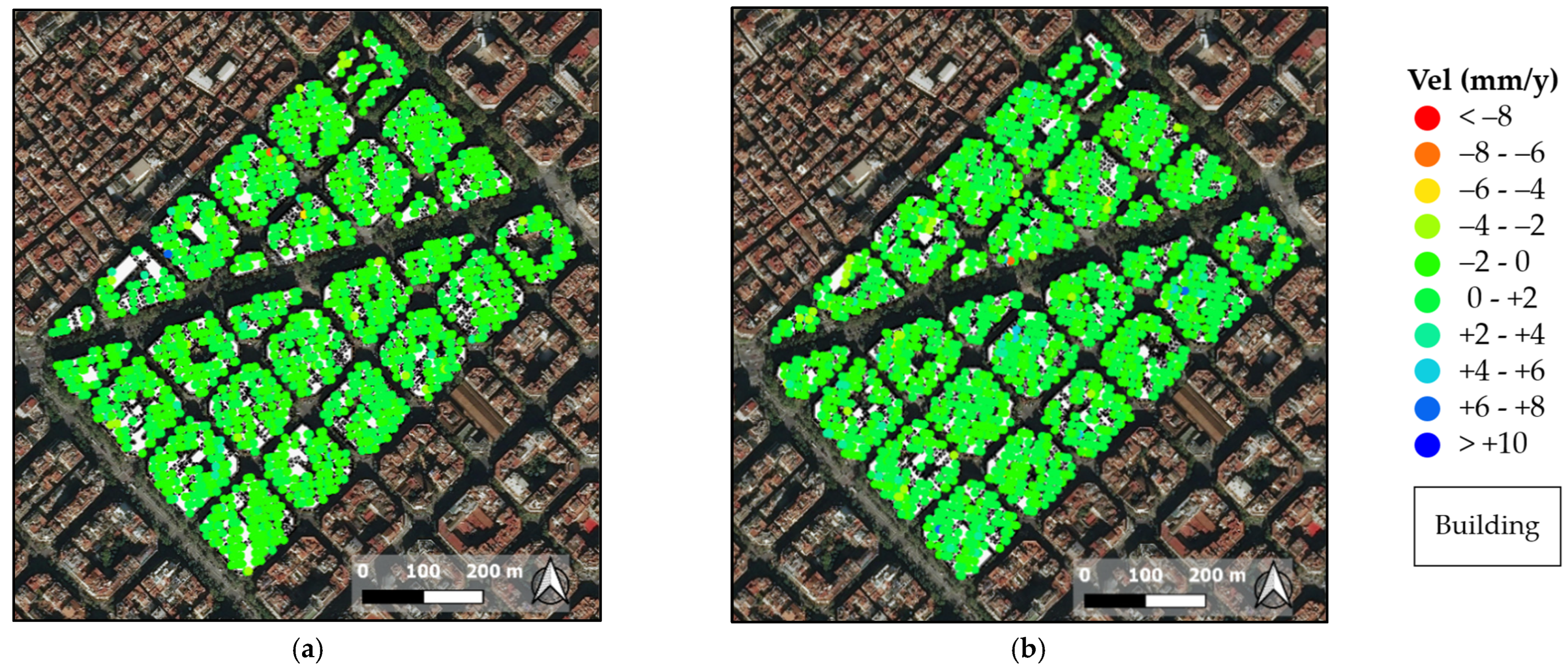
Then, for both orbits, the results of the ADAfinder tool are obtained (orange box of the flowchart), consisting in two maps: one with the ADA (a polygonal
ESRI shapefile), and one with the PSs contained in each ADA (a point
ESRI shapefile), as explained in
Section 2.2. These products are spatially superimposed to the polygons of buildings, obviously, as they are obtained from the PSs previously selected on the basis of them.
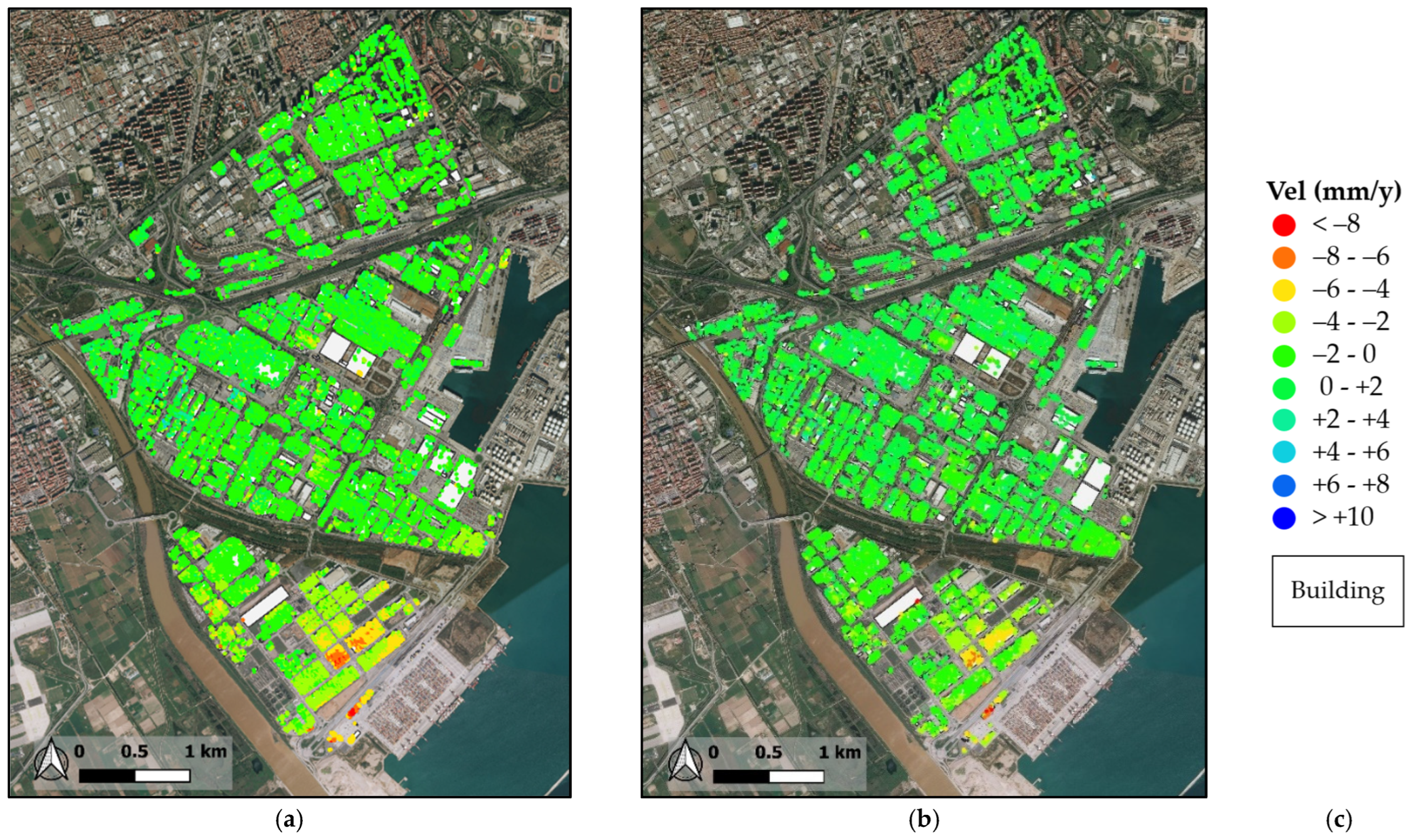
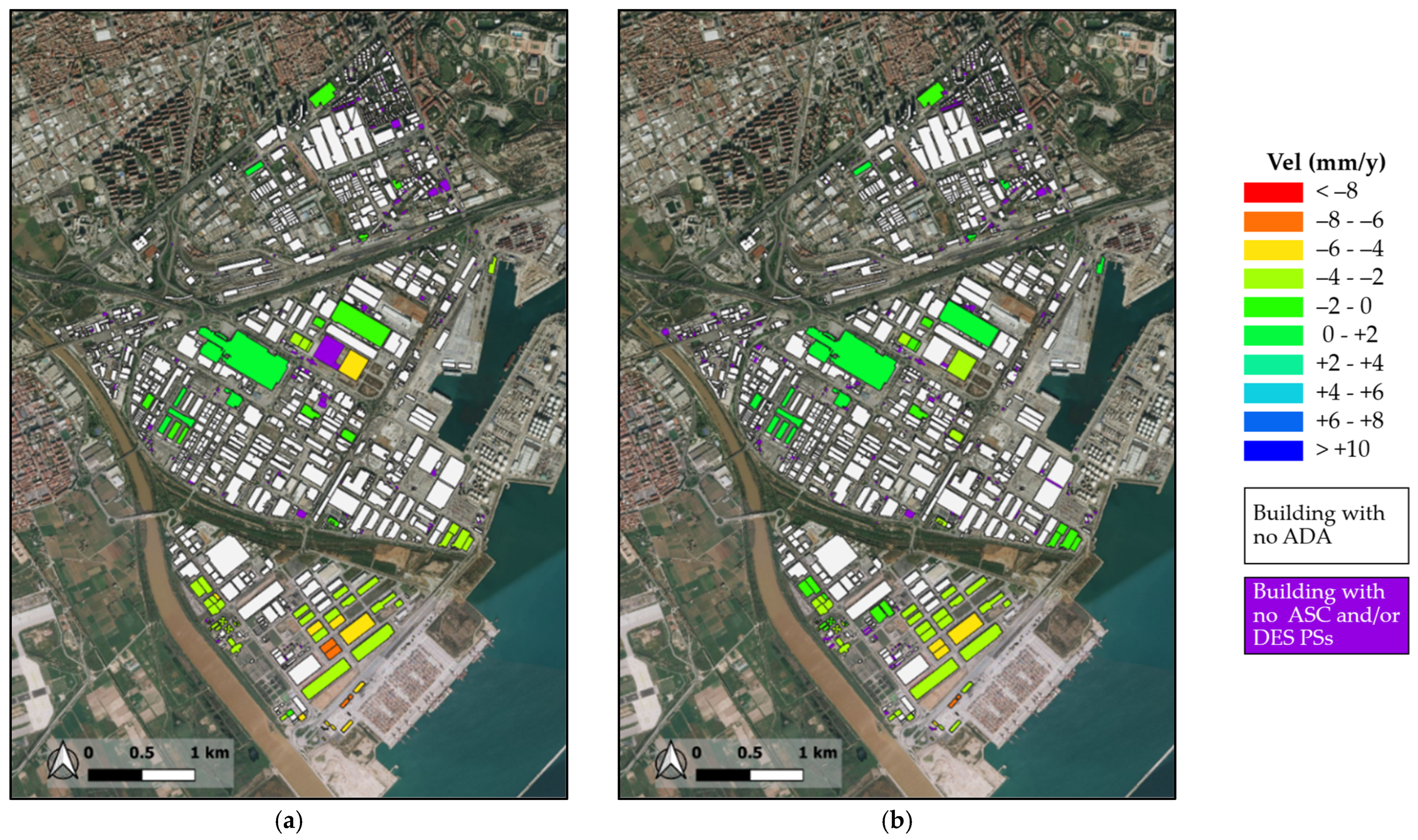
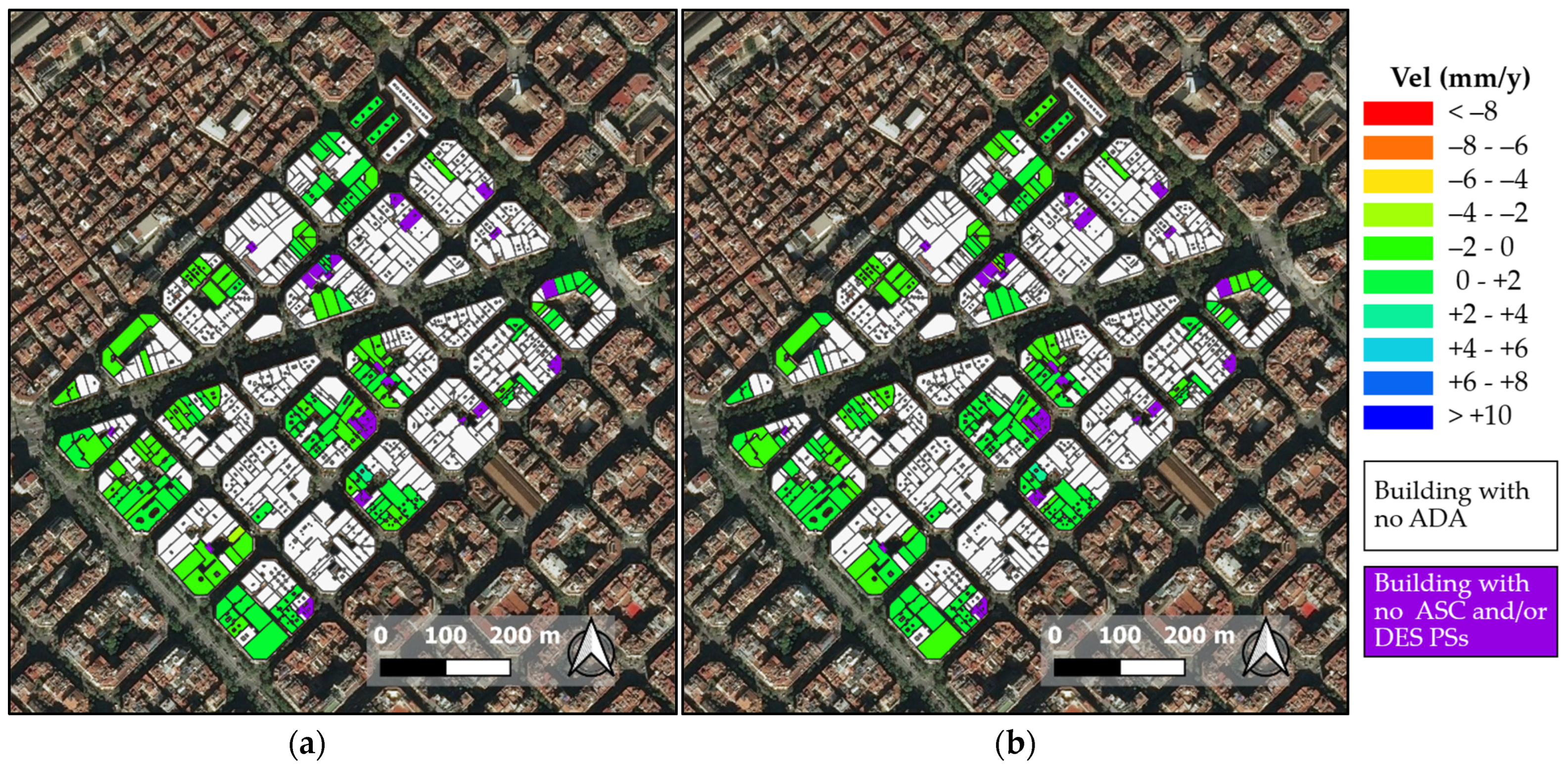
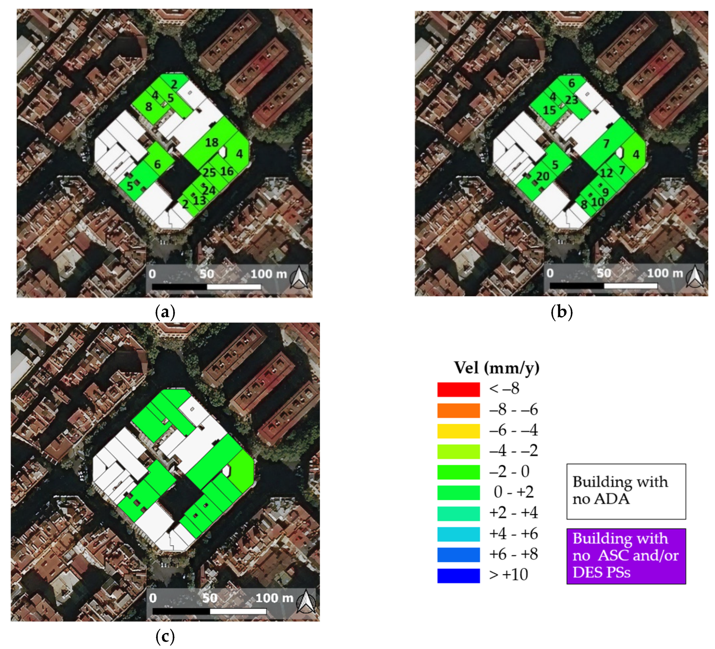
Finally, the ADAfinder results elaborated in order to obtain the definitive maps with information reclassified in function of the buildings, following the steps listed in the blue box of the flowchart. First of all, the ADA are overlapped to the buildings’ plans. The buildings not included in an ADA or a portion of an ADA are discarded. The remaining buildings, or portions of them, are classified as “unstable”. For them, two groups of “unstable” PSs are recognized: the group of ASC and the group of DES PSs. Then, for each building (with adequate numbers of PS), the average of the V
m and the σ of the ASC and DES PSs is computed only for the PSs inside the interested ADA. In this way, finally, only two values of V
m are associated to each building, representing the average of the mean deformation velocity along the line of sight (LoS) of the unstable PSs falling on the building itself: one along ASC (V
m,ASC) and one along DES (V
m,DES) orbits. At this step, an intersection of the results deriving from the ASC and DES datasets is performed to identify the buildings overlapped by at least one ADA from the ASC and one ADA from the DES dataset. The buildings not having both ASC and DES information are excluded from the following steps of the procedure, since the availability of both orbits is necessary for the estimation of the vertical and E-W mean deformation velocity components. Then, the vertical and E-W components of the mean deformation velocity for each building are estimated according to the formulas described in Talledo et al. [
15]. The north–south component cannot be calculated, due to the very low sensitivity of the InSAR to this displacement component, because of the approximately north–south orbit inclination of SAR satellites. All the operations included in the dashed red contour in
Figure 1 are done separately for each building included in an ADA.
The final maps give a preliminary identification of constructions potentially critical from a structural engineering point of view in terms of deformation, which needs a more accurate level of SHM.
The steps of the illustrated methodology can be implemented by combining simple operations to execute in QGIS and algorithms written in a code language (e.g., Matlab), as will be presented later.


