Estimating Nighttime PM_2.5 Concentration in Beijing Based on NPP/VIIRS Day/Night Band

Abstract

Nighttime PM_2.5 detection by remote sensing can expand understanding of PM_2.5 spatiotemporal patterns due to wider coverage compared to ground monitors and by supplementing traditional daytime detection. However, using remote sensing data to invert PM_2.5 at night is still challenging. Compared with daytime detection, which operates on sunlight, nighttime detection operates on much weaker moonlight and artificial light sources, complicating signal extraction. Moreover, as the attempts to sense PM_2.5 remotely using satellite data are relatively recent, the existing nighttime models are still not mature, overlooking many important factors such as stray light, seasonality in meteorological effects, and observation angle. This paper attempts to improve the accuracy of nighttime PM_2.5 detection by proposing an inversion model that takes these factors into consideration. The Visible Infrared Imaging Radiometer Suite/Day/Night Band (VIIRS/DNB) on board the polar-orbiting Suomi National Polar-orbiting Partnership (Suomi NPP) and National Oceanic Atmospheric Administration-20 (NOAA-20) was used to establish a nighttime PM_2.5 inversion model in the Beijing area from 1 March 2018 to 28 February 2019. The model was designed by first studying the effects of these factors through a stepwise regression, then building a multivariate regression model to compensate for these effects. The results showed that the impact of satellite viewing zenith angle (VZA) was strongest, followed by seasonality and moonlight. Total accuracy was measured using correlation coefficient (R) compared to ground measurements, achieving 0.87 over the urban area and 0.74 over the suburbs. Specifically, the proposed method works efficiently at subsatellite points, which in this case correspond to VZA from 0 and 5°. In spring, summer, autumn, and winter, the R reached 0.95, 0.93, 0.94, and 0.97 at subsatellite points in the urban area, while it was 0.88, 0.82, 0.85, and 0.77 in the suburbs.

1. Introduction

Since its reform and opening up, China has experienced severe air pollution resulting from the accelerating development of industry and cities [1]. As a political, economic, and technological center, Beijing has become one of the hardest-hit areas [2]. Studies have shown that inhalable particulate matter PM_2.5 is the primary pollutant [3], which disrupts the balance of atmospheric radiation, affects climate change, reduces visibility, and causes serious health problems [4,5,6,7]. Therefore, efficiently assessing temporal and spatial changes in PM_2.5 is critical for managing the environment and improving public health.

China established a PM_2.5 ground monitoring network in 2013. It accurately measures PM_2.5 in time. However, there exist two drawbacks. One is the high cost of monitoring devices and operating them. Another is the scattered and limited number of monitoring sites. Therefore, scholars have favored satellite remote sensing because of its high spatial resolution, cost effect, and repeatable measurement. It is gradually applied to estimate ground PM_2.5 values. Currently, the most popular approach is to use aerosol optical depth (AOD) to calculate the surface PM_2.5. AOD is a satellite derivative characterizing the comprehensive extinction effect of particulate matter in the atmosphere. These are some commonly used models: simple linear regression [8], multiple linear regression (MLR) [9,10], geographically weighted regression (GWR) [11], generalized additive model [12], mixed effects model (MEM) [13,14], two-stage model [15], and chemical transport model [16,17]. Furthermore, machine learning methods with strong nonlinear processing capabilities are also often used, such as random forest [18], extreme gradient boosting [19,20], and neural networks [21], etc.

Nevertheless, these studies aim at evaluating daytime PM_2.5. There are only a few studies on the retrieval of PM_2.5 at night by satellite remote sensing [22,23,24,25,26,27,28,29]. Two reasons mainly cause this situation. One is that there is no AOD product with high spatial resolution at night. The other is that the radiation transmission at night is relatively complex, including surface artificial light and natural light sources such as moonlight. What is more, artificial light changes over a long time. With the launch of nighttime remote sensing detectors in the visible light band, utilizing nighttime light (NTL) to monitor PM_2.5 has gradually attracted the attention of scholars in recent years. Li et al. [22] used the low light of the Defense Meteorological Satellite Program/Operational Linescan System (DMSP/OLS) from 9 October 2013 to 6 February 2014, and the PM_2.5 data measured by monitoring sites to build an inversion model using the backward neural network. Li et al. [30] adopted daytime AOD, combined the Normalized Difference Vegetation Index (NDVI), wind speed, and planetary boundary layer height to predict PM_2.5 in the northeastern United States using GWR. Wang et al. [23] first explored the feasibility of deriving surface PM_2.5 from the night visible light detected by VIIRS/DNB using an optical model in Atlanta, USA; Zhao et al. [24,25] and Li et al. [26] verified this method, finding it is also applicable to Beijing and Shanghai, China, respectively. Based on the “variance method” proposed by McHardy et al. [31], Fu et al. [27] used the radiance difference between pixels to solve the nighttime AOD and then estimated the concentration of PM_2.5. Zhang et al. [32] took Beijing–Tianjin–Hebei (BTH) as the research area. They constructed five different GWRs with the NTL of VIIRS/DNB and LJ1-01, AOD, and meteorological data to verify the feasibility of using NTL to estimate PM_2.5 in BTH. Recently, Wang et al. [28] proposed a method to invert surface PM_2.5 based on multi-source data, including monthly NTL of VIIRS, meteorological data, and topographic data, which provided a reference for PM_2.5 research.

Although some progress has been made in using NTL to estimate PM_2.5, some important influencing factors still have not been addressed. (1) The impact of moonlight. Most existing studies have either dropped the data with moonlight or directly ignored the impact of moonlight on model building. (2) Changes in quarterly impact factors. The majority of research uses the quarter as the research period or to divide the dataset. Then, the same input factors are used each quarter when constructing models. However, the factors affecting PM_2.5 in different seasons are diverse. (3) The angle effect of NTL. Several studies have shown that urban NTL has bidirectional reflectance distribution function (BRDF) characteristics [33,34]. Besides, different viewing paths affect the radiance of scattered light [35]. However, few existing studies have considered the impact of VZA on nighttime PM_2.5.

Among the widely used NTL products, VIIRS/DNB has higher space (2.7 to 0.75 km) and radiation resolution (6 to 14 bits) than DMSP/OLS. More importantly, it adds on-satellite calibration and solves the problem of pixel saturation in bright areas [36]. Therefore, we used NTL of VIIRS/DNB, first analyzing the moonlight’s impact on it, then selecting the impact factors quarterly, and using MLR to build a PM_2.5 inversion model. Finally, we explored the effect of VZA on utilizing NTL to calculate PM_2.5. The rest of this paper is structured as follows: Section 2 introduces the study area and the datasets used. Section 3 presents data preprocessing and methodology. Section 4 displays the results, evaluates model performance and discusses them. Section 5 summarizes our work.

2. Study Area and Data

2.1. Study Area

Beijing (39°26′–41°03′ N, 115°25′–117°30 E) is the capital of China, located in the northern part of the North China Plain, with an area of about 16,411 km² and an average elevation of 43.5 m. The terrain of Beijing shows a decreasing trend from northwest to southeast. Plains and mountains dominate the landscape. Mountains on three sides surround the urban area, which is adverse to atmospheric diffusion [37]. Beijing has a typical north-temperate semi-humid continental monsoon climate. Its summer is hot and rainy, winter is cold and dry, and spring and autumn are short. There are 16 districts under the city’s jurisdiction that have established 35 PM_2.5 monitoring stations (Figure 1). The government has taken measures such as moving out, shutting down polluting enterprises, and adjusting the energy structure of motor vehicles to control smog. These measures have already achieved excellent results. However, the concentration of PM_2.5 in Beijing is still relatively high. In 2018, the average annual concentration of PM_2.5 reached 51 μg/m³, which exceeded the national standard (35 μg/m³) by 46%. PM_2.5 is still the primary pollutant in the air, which threatens the health of millions of people.

2.2. Data

Our research period was from 1 March 2018 to 28 February 2019. We adopted three types of experimental data. (1). Ground site data: It was hourly measurement of PM_2.5 at monitoring sites. (2). Remote sensing data, including NTL of VIIRS/DNB, cloud cover layers (VCCLO), surface reflectance, and vegetation data. (3). Meteorological data, covering AOD, 2 m temperature, 2 m dew point temperature, surface pressure, evaporation, precipitation, 10 m u-component of wind, 10 m v-component of wind, and boundary layer height.

Table 1. Summary of datasets used in this study.

Source	Abbreviation	Content	Unit	Spatial Resolution	Temporal Resolution
BJMEMC 1	PM2.5	PM2.5	μg/m3	-	Hourly
VIIRS/SDR	NTL	Nighttime light	W/cm2·sr	750 m × 750 m	Daily
VIIRS/EDR	VCCLO	Cloud cover layers	-	6 km × 6 km	Daily
MOD09A1	Reflectance	Surface reflectance	-	500 m × 500 m	8-Day
MOD13A3	EVI	Enhanced Vegetation Index	-	1 km × 1 km	Monthly
EAC4	AOD	Total AOD at 550 nm	-	0.75° × 0.75°	3-h
ERA5	TEM	2 m temperature	K	0.1° × 0.1°	Hourly
	DTEM	2 m dew point temperature	K	0.1° × 0.1°	Hourly
	SP	Surface pressure	Pa	0.1° × 0.1°	Hourly
	ET	Evaporation	m	0.1° × 0.1°	Hourly
	PRE	Precipitation	m	0.1° × 0.1°	Hourly
	U-WS	10 m u-component of wind	m/s	0.1° × 0.1°	Hourly
	V-WS	10 m v-component of wind	m/s	0.1° × 0.1°	Hourly
	BLH	Boundary layer height	m	0.25° × 0.25°	Hourly

¹ Beijing Municipal Ecological and Environment Monitoring Center.

lists relevant information on the data used in this study.

2.2.1. Ground PM_2.5 Measurements

This study used the ground hourly measuring PM_2.5 concentration provided by the Beijing Municipal Ecological and Environment Monitoring Center (http://zx.bjmemc.com.cn/, accessed on 11 January 2022). As shown in Figure 1, monitoring sites established in Beijing fall into four types: 12 urban environmental assessment points (UEAP), 5 traffic pollution monitoring points (TPMP), 11 suburban environmental assessment points (SEAP), and 7 control points and regional points (CPRP). We removed the ZWY site from these sites due to perennial missing data. The distribution of monitoring sites in the whole area is uneven. The density of urban sites is relatively high, while sparse in the suburbs. If measuring PM_2.5 at each site remained unchanged for three consecutive hours due to possible instrument failure, we removed it as an anomaly [38].

2.2.2. Remote Sensing Data

This paper used two types of remote sensing data: VIIRS and moderate-resolution imaging spectroradiometer (MODIS).

• VIIRS

VIIRS is a crucial instrument carried on NPP and NOAA-20. It is a radiometer with a scanning width of about 3044 km (cross-track direction) [39]. VIIRS has 5 image bands (I band), 16 medium resolution bands (M band), and 1 panchromatic band (DNB), a total of 22 bands. DNB has a wide spectral range (500–900 nm), which uses three gain stages—low gain stage (LGS), medium gain stage (MGS), and high gain stage (HGS)—to achieve a wide dynamic range from day to night, with a monitoring range of 3 × 10⁻⁹ − 0.02 w/cm²·sr. To increase the signal, the time delay integration of the three gain stages has 1, 3, and 250 pixels, respectively [40]. This study used two datasets of VIIRS. One was the VIIRS/DNB Sensor Data Record (SDR) dataset, which contains two types of data: (1) the scientific data record (SVDNB) providing the radiance of NTL; (2) the geolocation content (GDNBO) that supplies the corresponding longitude, latitude, satellite viewing zenith angle, lunar zenith angle (LZA), and lunar phase angle (LPA). The other was the VIIRS Environmental Data Recording (EDR) dataset. It contains VCCLO, which uses cloud optical properties, cloud top parameters, and perform parallax correction data to output cloud products gridded to 6 km spatial resolution through spatial aggregation. With an accuracy of up to 98% [41], VCCLO contains geographical locations, several types of clouds, and summed cloud cover (SCC). We applied SCC in the research. All data were from the NOAA’s Comprehensive Large Array-Data Stewardship System (https://ncc.nesdis.noaa.gov/VIIRS/, accessed on 13 April 2022).

2.

MODIS

MOD09A1 and MOD13A3 are MODIS Level-3 products, both projected in sinusoidal. MOD09A1 has a total of 7 bands, providing the spectral reflectance of the surface. Each pixel selects the best Level-2 observation based on high coverage, cloud-free, and aerosol loading over eight days. To obtain the surface albedo of the visible light band at night, we selected Band 1 (620~670 nm), Band 2 (841~876 nm), and Band 4 (545~565 nm) channels to calculate the surface albedo according to Equation (1) [42].

$${\rho }_a=\frac{{\displaystyle \sum _{i=1,2,4}{\displaystyle {\int }_{{\lambda }_{i,1}}^{{\lambda }_{i,2}}\rho ({\lambda }_i)SRF({\lambda }_i)d{\lambda }_i}}}{{\displaystyle \sum _{i=1,2,4}{\displaystyle {\int }_{{\lambda }_{i,1}}^{{\lambda }_{i,2}}SRF({\lambda }_i)d{\lambda }_i}}}$$

(1)

where ${\rho }_a$ is the surface albedo of DNB, ${\lambda }_{i,1}$, and ${\lambda }_{i,2}$ are the minimum and maximum wavelengths of the band $i$, respectively. ${\lambda }_i$ is the wavelength in band $i$. $\rho ({\lambda }_i)$ is the reflectance at wavelength ${\lambda }_i$, and $SRF({\lambda }_i)$ is the response of DNB at ${\lambda }_i$. MOD13A3 provides two vegetation indices: Normalized Difference Vegetation Index and Enhanced Vegetation Index. Compared with NDVI, EVI minimizes the background variation of the canopy and maintains sensitivity to dense vegetation conditions, so we chose EVI for this study. Both datasets came from Level-1 and Atmosphere Archive & Distribution System Distributed Active Archive Center (https://ladsweb.modaps.eosdis.nasa.gov/search/, accessed on 24 April 2022).

2.2.3. Meteorological Data

We acquired AOD from EAC4 provided by the European Centre for Medium-Range Weather Forecast (https://ads.atmosphere.copernicus.eu/, accessed on 19 April 2022). At the same time, temperature, dew point temperature, air pressure, evaporation, precipitation, u-component of wind, and v-component of wind data came from the ERA5-Land reanalysis product. Using the temperature and the dew point temperature, we calculated the relative humidity (RH, unit: %) using Equation (2).

$$RH=\frac{e}{es}\times 100,$$

(2)

where $e$ is the vapor pressure, the computing formula is as in Equation (3), $es$ is the saturated vapor pressure, and the formula is as in Equation (4).

$$e=6.1078\times {10}^{\frac{7.5\times (TD-273.15)}{237.3+(TD-273.15)}},$$

(3)

$$es=6.1078\times {10}^{\frac{7.5\times (T-273.15)}{237.3+(T-273.15)}},$$

(4)

where TD represents dew point temperature, and T represents temperature. Then, wind speed and wind direction were calculated through U-WS and V-WS. Finally, we converted the units of surface pressure from Pa to hPa, and altered the units of evaporation and precipitation from m to mm. The Climate Change Service (https://cds.climate.copernicus.eu/, accessed on 8 April 2022) provided all the meteorological data.

3. Method

Using NTL of VIIRS/DNB to estimate PM_2.5 at night was divided into three key steps. (1) Data preprocessing, including selection of observations by cloud mask, moonlight correction, and data integration. (2) Model development: Firstly, we selected the appropriate pixel-scale data to characterize the radiance of the target area’s light. Next, monitoring sites were screened for model building. Then, we adopted a stepwise regression model to choose the influencing factors of PM_2.5 in different seasons. Finally, a multivariate regression model was applied to determine the estimated PM_2.5. (3) Model validation: We used ten-fold cross-validation to evaluate the performance of our model.

3.1. Data Preprocessing

3.1.1. Selection of Observations by Cloud Mask

DNB is imaged in the visible and near-infrared bands, seriously affected by clouds. Figure 2a,b shows two DNB images with a clear sky, no moon (LZA > 118°), a similar VZA, and the PM_2.5 in (a) is lower than that in (b). The discrepancy was that (a) contains clouds over a large area, while (b) has few clouds. The figure shows that the cloud layer seriously interferes with the DNB image, so it is essential to filter cloud contamination.

In this study, we chose VCCLO as cloud mask. Then, VCCLO’s SCC was applied to select observations without cloud. In Figure 2c,d are the VCCLO corresponding to (a) and (b). We calculated the entire area’s cloud coverage according to Beijing’s vector boundary line. If it reached 50%, the DNB image was directly discarded. Otherwise, we took the image’s cloudless (SCC = 0) pixels.

3.1.2. Moonlight Correction

The radiance received by satellites at night primarily comes from two sources: one is surface city light, and the other is moonlight. The city light does not change significantly in the short term, but the moonlight changes periodically (new moon to full moon to new moon). To evaluate the effect of moonlight on inverting surface PM_2.5 from NTL, we performed moonlight correction processing on the radiance of DNB.

As stray light, moonlight comes from the reflection of sunlight through the lunar surface to the Earth’s surface and then through the atmosphere to the pupil of the satellite. Moonlight irradiance is predominantly affected by four factors: solar radiance, lunar spectral reflectance, lunar phase angle, and geometric distance between Sun/Moon/Earth. In this study, the dynamic lunar hyperspectral irradiance model (MT2009) proposed by Miller et al. [43] was used to calculate the lunar irradiance at the target time. Then, we used Equation (5) to calculate the radiance of moonlight observed by satellite [33].

$$R_m=\frac{E_m\cos ({\theta }_m)T_{\downarrow }(\tau ,{\theta }_{\upsilon }){\rho }_{\alpha }{T}_{\uparrow }(\tau ,{\theta }_{\upsilon })}{\pi (1-\alpha ({\theta }_m){\rho }_{\alpha })}+L_{path},$$

(5)

where $R_m$ is the moonlight radiance at the sensor aperture, $E_m$ is the lunar irradiance, ${\theta }_m$ is the zenith angle of the moon, $T_{\downarrow }(\tau ,{\theta }_{\upsilon })$ is the total transmittance of the moonlight to the surface path, $T_{\uparrow }(\tau ,{\theta }_{\upsilon })$ is the total transmittance from the surface to the satellite path, ${\rho }_{\alpha }$ is the surface Lambertian albedo (see Equation (1) for the calculating method), $\alpha ({\theta }_m)$ is the atmospheric apparent albedo, $L_{path}$ is the path radiance from lunar illumination of the atmosphere. $T_{\downarrow }(\tau ,{\theta }_{\upsilon })$, $T_{\uparrow }(\tau ,{\theta }_{\upsilon })$, $\alpha ({\theta }_m)$, $L_{path}$ was calculated by Moderate Resolution Atmospheric Transmission 5 (MODTRAN5). Before using MODTRAN5 to calculate parameters, we analyzed the sensitivity of MODTRAN5 to primary input data. We adopted the control variable method to alternately input different values of CO₂, water vapor, LZA, VZA supplementary angle, AOD, relative azimuth angle, and moon phase angle, then observed the effect of each variable on the output transmittance. We found that MODTRAN5 was not sensitive to constant gases such as CO₂ or water vapor when calculating the total transmittance. Nevertheless, it was susceptible to AOD at 550 nm and input zenith angle (downward transmittance: LZA; upward transmittance: VZA). Therefore, we chiefly considered AOD and LZA/VZA in the calculation. The LZA/VZA was gained from DNB images. For AOD, we acquired the total optical thickness of particles at 550 nm from the EAC4 dataset after using kriging interpolation. Finally, the lunar radiance at the pupil of the satellite was obtained and subtracted from the satellite observations.

3.1.3. Data Integration

Since the original projections and spatial resolutions of various data types in the dataset were different, we uniformly transferred them to the WGS84 coordinate system. Then, the linear interpolation was applied to resample these data to 750 m. Thus, they were kept consistent with DNB’s spatial resolution, which is beneficial for matching NTL. We used longitude and latitude to complete data pairing. This study applied the nearest neighbor method for all independent variables. Precisely, for NTL, meteorological data, and EVI et al., we extracted the closest pixel value of the monitoring site and assigned the corresponding PM_2.5. Each data record corresponded to a particular day and place, and the data record was discarded when any data were missing. Finally, there were a total of 5288 matched data pairs.

3.2. Model Development

3.2.1. Pixel Scale Selection

To obtain the radiance needed to accurately assess the PM_2.5 of monitoring sites, we needed to select the pixel scale at first. A relationship between surface PM_2.5 and satellite-observed radiance was deduced [23] as shown in Equation (6).

$$\frac{{PM}_{2.5}f(\mathrm{RH})}{\mu }=a_0-\ln (\mathrm{I})-a_1\times W-a_2\times Ps,$$

(6)

where PM_2.5 is the mass concentration of surface PM_2.5, f(RH) is the relative humidity correction factor for aerosol size and refractive index, μ is the cosine of the VZA, $a_0$, $a_1$, and $a_2$ are the linear coefficients, I is the radiance extracted from DNB, ln(I) is the natural logarithm of I, $W$ is water vapor, $Ps$ is surface pressure. In order to verify the effect of correcting humidity in estimating PM_2.5 in Beijing, we analyzed the relationship between humidity corrected PM_2.5 (PM_2.5f(RH)/μ), humidity uncorrected PM_2.5 (PM_2.5/μ), and ln(I). The results showed that the latter was more closely related to ln(I). Therefore, in this study, we did not perform correcting humidity on PM_2.5 but included RH/μ in the multiple regression variable factors. We adopted the Pearson coefficient shown in Equation (7) to perform a bivariate correlation analysis between PM_2.5/μ and ln(I).

$$r=\frac{{\displaystyle {\sum }_{i=1}^n(x_i-\overline{x})(y_i-\overline{y})}}{\sqrt{{\displaystyle {\sum }_{i=1}^n{(x_i-\overline{x})}^2{(y_i-\overline{y})}^2}}},$$

(7)

where n is the number of samples, $x_i$ and $y_i$ are the actual values of the data, $\overline{x}$ and $\overline{y}$ are the mean of the data. The value range of $r$ is (−1,1). When $\left|r\right|$ is closer to 1, the correlation between $x$ and $y$ is higher. In general, when $\left|r\right|$ ≥ 0.8, they are regarded as highly correlated; when 0.5 ≤ $\left|r\right|$ < 0.8, they are regarded as moderately correlated; when 0.3 ≤ $\left|r\right|$ < 0.5, they are regarded as lowly correlated; when $\left|r\right|$ < 0.3, it means that the correlation between the two variables is very weak.

Table 2. Correlation coefficients between PM_2.5/μ and ln(I) at different pixel scales for 34 ground monitoring sites: ln(I) is the natural logarithm of radiance extracted from DNB.

Site	1 × 1 Pixel	3 × 3 Pixels	5 × 5 Pixels
DS	−0.03	−0.52	−0.55
TT	0.11	−0.08	−0.41
GY	−0.44	−0.63	−0.65
WSXG	−0.03	−0.35	−0.45
ATZX	−0.23	−0.54	−0.61
NZG	−0.12	−0.51	−0.63
WL	−0.3	−0.54	−0.51
BBXQ	−0.09	0.05	0.07
FTHY	−0.5	−0.42	−0.29
YG	−0.3	−0.41	−0.37
GC	−0.32	−0.69	−0.63
QM	−0.37	−0.62	−0.59
YDMN	0	−0.13	−0.29
XZMB	−0.13	−0.31	−0.62
NSH	−0.38	−0.53	−0.51
DSH	−0.21	−0.38	−0.38
FS	−0.62	−0.64	−0.46
DX	−0.11	−0.06	0.03
YZ	−0.57	−0.56	−0.54
TZ	−0.55	−0.57	−0.59
SY	−0.38	−0.57	−0.53
CP	−0.55	−0.7	−0.63
MTG	−0.27	−0.6	−0.66
PG	−0.67	−0.72	−0.7
HR	−0.5	−0.54	−0.56
MY	−0.32	−0.56	−0.6
YQ	−0.38	−0.64	−0.64
DL	0.16	0.18	0.18
BDL	0.18	0.14	0.2
MYSK	0.21	0.22	0.23
DGC	0.2	0.05	−0.07
YLD	−0.36	−0.1	0.01
YF	0.12	0.25	0.2
LLH	0.07	−0.01	0.04
Mean	−0.23	−0.35	−0.37

At each site, the largest value is in bold.

lists correlation coefficients between PM_2.5/μ and ln(I) in 34 ground monitoring sites with 1 × 1 pixel (about 0.75 × 0.75 km), 3 × 3 pixels (about 1.5 × 1.5 km), and 5 × 5 pixels (about 3.75 × 3.75 km), respectively. The most significant coefficients at each site were in bold. The experimental comparison showed that the correlation between PM_2.5/μ and ln(I) within 5 × 5 pixels centered on the site was generally the highest. Therefore, we extracted the average ln(I) over a 5 × 5 pixel range centered on the site.

3.2.2. Sites Selection

We analyzed the correlation coefficient of PM_2.5/μ and ln(I) at each site by season and synchronously counted each site’s annual average I for the following reasons. One was to explore the feasibility of multiple linear regression in this study. Another was to filter out some sites unsuitable for this method. Figure 3 shows scatter plots of PM_2.5/μ and ln(I) for the DS site in the urban area and the FS site in the suburbs.

Table 3. Correlation coefficients between PM_2.5/μ and ln(I) for each season at each site: I_mean is the annual mean of radiance at each site in units of nW/cm²·sr.

Site	Spring	Summer	Autumn	Winter	Imean
DS	−0.56	−0.65	−0.53	−0.45	47.87
TT	−0.53	−0.46	−0.36	−0.27	44.77
GY	−0.65	−0.81	−0.62	−0.52	40.61
WSXG	−0.41	−0.46	−0.5	−0.41	42.26
ATZX	−0.58	−0.79	−0.55	−0.52	48.47
NZG	−0.65	−0.73	−0.65	−0.47	43.85
WL	−0.52	−0.61	−0.47	−0.42	27.95
BBXQ 1	0.11	0.13	0.05	0	11.6
FTHY	−0.26	−0.3	−0.23	−0.37	35.22
YG	−0.27	−0.44	−0.42	−0.34	12.66
GC	−0.61	−0.74	−0.54	−0.62	35.45
QM	−0.64	−0.71	−0.58	−0.43	60.15
YDMN	−0.29	−0.28	−0.32	−0.26	35.87
XZMB	−0.58	−0.74	−0.58	−0.58	36.68
NSH	−0.5	−0.54	−0.45	−0.53	44.55
DSH	−0.46	−0.3	−0.35	−0.41	32.84
FS	−0.29	−0.54	−0.5	−0.51	19.65
DX 1	0.35	0.26	−0.2	−0.27	13.98
YZ	−0.45	−0.7	−0.61	−0.4	32.04
TZ	−0.61	−0.61	−0.63	−0.51	38.48
SY	−0.38	−0.69	−0.53	−0.51	30.31
CP	−0.62	−0.75	−0.66	−0.5	26.25
MTG	−0.63	−0.81	−0.57	−0.62	26.38
PG	−0.66	−0.87	−0.62	−0.64	20.43
HR	−0.53	−0.54	−0.52	−0.65	22.49
MY	−0.62	−0.72	−0.57	−0.47	27.72
YQ	−0.6	−0.75	−0.6	−0.59	21.63
DL 1	0.36	0.37	0.06	−0.08	2.23
BDL 1	0.24	0.39	0.02	0.14	2.79
MYSK 1	0.39	0.6	0.14	−0.2	1.42
DGC 1	0.06	0.2	−0.26	−0.28	6.33
YLD 1	0.14	0.28	−0.21	−0.19	4.39
YF 1	0.39	0.53	0.1	−0.23	6.96
LLH1	0.38	0.3	−0.26	−0.24	4.58

¹ Sites were not contained in constructing models.

lists all analytical results. Our experiment showed that the radiance in the urban area was generally higher than that in the suburbs, while that of SEAP was usually higher than that of CPRP. Commonly, PM_2.5/μ was negatively correlated with ln(I), mostly higher than 0.5. However, few sites had weak negative or positive correlations between PM_2.5/μ and ln(I). They were the BBXQ site in the urban area, DX in the suburbs, and seven CPRPs. These sites had a common feature: the annual I was very low (1.42–13.98 nW/cm²·sr). The annual I of CPRP maintained within 7 nW/cm²·sr, including three sites’ I below the threshold of DNB (3 nW/cm²·sr). The reason for this situation was that in the low light area, the NTL’s radiation of the pixel was feeble at night, and a large ratio of radiance received by the satellite comes from the scattered radiation of the surrounding background pixels. When PM_2.5 is higher, the scattering effect of the atmosphere is more substantial. The corresponding background radiance also increases, increasing the radiance received by the satellite. Therefore, PM_2.5/μ positively correlated with ln(I). In the high light area, the radiance received by the satellite mainly comes from the direct radiation of the pixel rather than the surrounding pixels’ scattered radiation. When PM_2.5 is higher, the scattering effect of the atmosphere is more robust. Then, the direct radiation loss of the pixel is more serious, resulting in a decrease in radiance received by the satellite. The results were consistent with the experimental results of Chen et al. [29] in Huai’an City, Jiangsu Province, China. We would not consider the nine sites for accuracy when constructing models. Meanwhile, considering the discrepancy in NTL and atmospheric conditions between the urban area and the suburbs, we would divide the sites into urban and suburban datasets according to geographic location.

3.2.3. Variables Selection

To decrease multicollinearity among variables, reduce redundancy of input data, and simultaneously explore the differences in the influencing factors of PM_2.5 estimated by NTL in each quarter, we used the forward approach of stepwise regression to select quarterly independent variables in the urban area and the suburbs, respectively. The main steps of the method were as follows:

Step 1: We established a univariate regression model with the n-regression independent variables $X_1,X_2,\dots ,X_n$, and the dependent variable $Y$, respectively, as shown in Equation (8).

$$Y={\alpha }_0+{\alpha }_i{\mathrm{X}}_i+\epsilon ,i=1,2,\dots ,n,$$

(8)

where ${\alpha }_0$ is a constant, ${\alpha }_i$ is the fitting coefficient of the variable, $\epsilon$ is the random error. Then, the F test statistic’s value of each variable’s corresponding fitting coefficient was calculated and the maximum value was recorded as $F_{l1}{}^{\prime }$. For the given significant level $\alpha$, we recorded the corresponding critical value as $F_1$. If $F_{l1}{}^{\prime }$ ≥ $F_1$, $X_{l1}$ was introduced into the regression model, then we denoted $L_1$ as the index set of the selected variables.

Step 2: A binary regression model of dependent variable $Y$ and independent variable subset $\{X_{l1},X_1\},\dots ,\{X_{l1},X_{l1-1}\},\{X_{l1},X_{l1+1}\},\dots ,\{X_{l1},X_n\}$ was established, with a total number of n–1. Similarly, we calculated the F test statistic’s value of the variable’s coefficient, and recorded the maximum value as $F_{l2}{}^{\prime }$. For the given significant level $\alpha$, the corresponding critical value was recorded as $F_2$. When $F_{l2}{}^{\prime }$ ≥ $F_2$, we introduced $X_{l2}$ into the regression model, then denoted $L_2$ as the index set of the selected variables.

Step 3: We repeated step 2 until no more variable could be introduced after experimenting—each time, an independent variable not included in the model was selected.

Ten types of data were selected as input factors in this study: ln(I), RH/μ, SP, ET, PRE, WS, WD, BLH, TEM, and EVI. We also selected each site’s annual average ln(I) as the input factor to eliminate the disparity in the radiance of various sites. Then, a stepwise regression was applied to screen out the variables closely related to the dependent variable PM_2.5/μ in each quarter. Next, we used these variables to establish a multivariate regression model.

Table 4. The variables selected for modeling each season in the urban area and in the suburbs.

Variable	Urban Area				Suburb
	Spring	Summer	Autumn	Winter	Spring	Summer	Autumn	Winter
ln(I)	√	√	√	√	√	√	√	√
Mean ln(I)	√	√	√	√	√	√	√	√
RH/μ	√	√	√	√	√	√	√	√
SP	√	√		√	√		√
ET	√	√	√	√	√	√	√	√
PRE		√	√	√		√	√
WS		√	√	√		√	√	√
WD		√	√			√		√
BLH	√	√	√	√	√	√
TEM	√			√			√
EVI	√			√	√		√	√

“√” represents the variable is selected in corresponding season.

shows the selected variables in urban and suburban areas. We found changes in impact factors of estimating nighttime PM_2.5 in each season. Concurrently, changes also existed in impact factors for the urban area and the suburbs in the same season. Particularly, ln(I), mean ln(I), RH/μ, and ET were selected in four seasons of both the urban area and the suburbs, indicating that the four variables play an essential role in estimating PM_2.5 at night. WS was selected in summer, autumn, and winter but not in spring. This result was due to low WS with no significant change in spring. Similar results existed for other variables such as SP, PRE, BLH, TEM, and EVI. We think the variables’ discrepancy results from seasonal and regional differences in the atmosphere.

3.2.4. Multivariate Regression Model Building

We utilized the variables selected in Section 3.2.3 to construct a multivariate regression model, as shown in Equation (9). Then, the least squares method was used to solve it.

$$y=w_0+w_1{x}_1+\dots +w_m{x}_m,$$

(9)

where $w_0$ is the intercept, $x_1,\dots x_m$ represent m input variables, $w_1,\dots w_m$ represent the weight of m variables. The output variables, input variables, and weights were expressed as matrices shown in Equations (10)–(12), respectively.

$$Y={(y_1,\dots ,y_k)}^T$$

(10)

$$X=\left[\begin{array}{cccc}1& x_1^1& \dots & x_m^1\\ 1& x_1^2& \dots & x_m^2\\ \dots & \dots & \dots & \dots \\ 1& x_1^k& \dots & x_m^k\end{array}\right]$$

(11)

$$W={(w_0,w_1,\dots ,w_m)}^T$$

(12)

where k represents the number of data groups, and $x_m^k$ represents the mth variable of the kth data group. Then, the loss function was constructed as shown in Equation (13).

$$J={\displaystyle \sum _{i=1}^k{(y_i-\widehat{y_i})}^2}$$

(13)

Finally, we obtained the weight matrix by minimizing the loss function J, as shown in Equation (14).

$$W={(X^{T}X)}^{-1}{X}^{T}Y={({\displaystyle \sum _{i=1}^k{x}_i}{x}_i^T)}^{-1}({\displaystyle \sum _{i=1}^k{x}_i}{y}_i),$$

(14)

3.3. Model Validation

Referring to previous studies [13,20,32], we used ten-fold cross-validation to evaluate our method. The general ten-fold cross-validation was to randomly divide all the samples into ten groups, with each subsample accounting for about 10% of the total dataset. Then, nine subsamples were selected each time to fit the model, and the remaining subsample was estimated using the fitting model. We repeated this ten times until each subsample had been validated. The model’s overall performance was evaluated by the difference between the measured and estimated values. We measured the model performance by R, mean bias (MB), mean absolute error (MAE), and root mean squared error (RMSE), as shown in Equations (15)–(18).

$$R=\frac{{\displaystyle \sum _{i=1}^n(P{M}_{2.5(i)}^{obs}-\overline{P{M}_{2.5}^{obs}})(P{M}_{2.5(i)}^{est}-\overline{P{M}_{2.5}^{est}})}}{\sqrt{{\displaystyle \sum _{i=1}^n{(P{M}_{2.5(i)}^{obs}-\overline{P{M}_{2.5}^{obs}})}^2}}\sqrt{{\displaystyle \sum _{i=1}^n{(P{M}_{2.5(i)}^{est}-\overline{P{M}_{2.5}^{est}})}^2}}},$$

(15)

$$MB=\frac{1}{n}|{\displaystyle \sum _{i=1}^n(P{M}_{2.5(i)}^{obs}-P{M}_{2.5(i)}^{est}})|$$

(16)

$$MAE=\frac{1}{n}{\displaystyle \sum _{i=1}^n|P{M}_{2.5(i)}^{obs}-P{M}_{2.5(i)}^{est}}|$$

(17)

$$RMSE=\sqrt{\frac{1}{n}{\displaystyle \sum _{i=1}^n{(P{M}_{2.5(i)}^{obs}-P{M}_{2.5(i)}^{est})}^2}}$$

(18)

where n is the number of samples, $P{M}_{2.5(i)}^{obs}$ and $P{M}_{2.5(i)}^{est}$ are the observed PM_2.5 and estimated PM_2.5 of the ith sample, and $\overline{P{M}_{2.5}^{obs}}$ and $\overline{P{M}_{2.5}^{est}}$ correspond to the mean of observed PM_2.5 and estimated PM_2.5, respectively.

4. Results and Discussion

In this part, we mainly conducted four works. The first was to analyze the relationship between daily PM_2.5 and mean PM_2.5 at satellite transit time day and night. Then, descriptive statistics analyses were performed for all quasi-input and output variables. Next, we explored the effect of moonlight on NTL’s inversion of the surface PM_2.5. Finally, the performance of the proposed model was described.

4.1. Collaboration between Nighttime PM_2.5 and Daytime PM_2.5

To explore whether the nighttime PM_2.5 estimated utilizing DNB can cooperate with the daytime PM_2.5 estimated by remote sensing to evaluate daily PM_2.5, we analyzed the relationship between hourly measured PM_2.5 at the satellite overpass time and daily measured PM_2.5 in our study period. The satellites usually used to estimate surface PM_2.5 are Terra, Aqua, and NPP. Generally, the data of Terra and Aqua at 10:30 and 13:30 China Standard Time (CST), respectively, were selected to study daytime PM_2.5, and the data of NPP at 1:30 CST were selected to study nighttime PM_2.5. Considering the calculation method of PM_2.5 by ground monitoring sites and only hourly PM_2.5 being provided, we analyzed correlation coefficients between daily PM_2.5 and hourly PM_2.5 at 2:00 CST, 11:00 CST, and 14:00 CST in each season, respectively.

Table 5. Correlation coefficients between daily measured PM_2.5 and hourly measured PM_2.5 at satellite overpass time: 2:00 CST, 11:00 CST, and 14:00 CST represent the transit time of NPP, Terra, and Aqua, respectively, which are commonly used to estimate PM_2.5.

Time	Spring	Summer	Autumn	Winter	Mean
2:00 CST	0.84	0.79	0.83	0.8	0.82
11:00 CST	0.92	0.9	0.94	0.84	0.9
14:00 CST	0.93	0.85	0.94	0.83	0.89

At each column, the largest value is in bold.

presents the analysis results. We found the degree of correlation between PM_2.5 at three moments and its daily mean in the following order: 11:00 CST > 14:00 CST > 2:00 CST.

Then, we analyzed the relationship between the mean of PM_2.5 at 2:00 CST and 11:00 CST (represented as hourly PM_2.5 in figures) and the daily PM_2.5. Figure 4 shows the corresponding scatterplots. The results showed that the mean PM_2.5 of NPP and Terra at 2:00 CST and 11:00 CST transit time and the daily PM_2.5 were highly correlated, with correlation coefficients of 0.97, 0.94, 0.97, and 0.93 in four quarters, which was closer to the daily PM_2.5 than the PM_2.5 of NPP, Terra, and Aqua alone at overpass times. It showed that using DNB to estimate nighttime PM_2.5 can cooperate with daytime PM_2.5 inverted by remote sensing, then help to make a more reasonable assessment of daily PM_2.5. The experimental results also demonstrated that the annual PM_2.5 measured by 34 ground monitoring sites in Beijing was 55.23 μg/m³. Seasonal PM_2.5 in spring, summer, autumn, and winter was 72.81 ± 1 μg/m³, 43.54 ± 0.46 μg/m³, 50.92 ± 0.92 μg/m³, and 53.65 ± 0.93 μg/m³. These differences can be attributed to existing seasonal changes in emissions and meteorological conditions.

4.2. Descriptive Statistics

Figure 5 shows histograms of all variables represented as frequency distributions. We performed statistical analysis quarterly.

Table 6. Descriptive statistics for variables: Std is short for standard deviation.

Variable	Min	Max	Mean	Midian	Std
PM2.5 (μg/m3)	1.00	410.00	46.82	33.00	45.16
Radiance (W/cm2·sr)	5.36 × 10−9	9.25 × 10−8	3.45 × 10−8	3.38 × 10−8	1.27 × 10−8
Relative humidity (%)	9.84	101.4	58.88	58.85	23.21
Surface pressure (hPa)	923.77	1041.45	1006.32	1009.22	17.44
Evaporation (mm)	0.00	5.24	1.19	0.84	1.26
Precipitation (mm)	0.00	10.93	0.16	0.00	0.95
Wind speed (m/s)	0.03	5.10	1.56	1.35	1.01
Wind direction (°)	0.01	359.95	232.62	280.61	114.54
Boundary layer height (m)	11.38	1614.31	140.59	41.37	263.69
Temperature (K)	253.77	302.18	278.96	276.54	11.05
EVI (unitless)	0.05	0.41	0.15	0.15	0.07

summarizes descriptive statistics of variables (e.g., minimum, maximum, mean, median, standard deviation). Figure 5 displays that PM_2.5 approximately distributed log-normally. Moreover, the PM_2.5 in spring and autumn was higher than that in summer and winter. The radiance distributed normally; it was the largest in winter, the smallest in spring, and similar in summer and autumn.

Regarding the relative humidity, in winter it kept relatively dry and mostly low, while overall humidity increased sequentially in spring, autumn and summer. The general trend of surface pressure was: summer < spring < autumn < winter, which was the inverse of the temperature’s trend. This result is attributable to the highest summer temperature; then, the gas distributes most discretely, resulting in the smallest surface pressure. In winter, the temperature stayed the lowest, and the gas was squeezed in the low sky, generating the highest surface pressure. Evaporation showed the same trend as temperature: winter < autumn < spring < summer. Generally, the higher the temperature, the greater the evaporation from the surface and vegetation.

With less precipitation all year round, Beijing kept dry. It had significant rainfall only in summer throughout the year. There existed breezes with northwesterly winds in all seasons. Furthermore, the wind speed in winter was relatively high. The planetary boundary layer height at night remained relatively stable, most of which stayed within 172 m. The enhanced vegetation index order was winter < spring < autumn < summer. The reason is that winter is cold, resulting in many plants withering. In spring, everything recovers, and plants begin to grow. Then, a lush state is reached in summer. After the arrival of autumn, the plants begin the process of shedding leaves and returning to their roots.

4.3. The Result of Correcting Moonlight

When LZA < 118° and LPA < 90°, we corrected moonlight from the radiance observed by the satellite.

Table 7. Correlation coefficients between PM_2.5/μ and ln(I), ln(I′) for 34 sites: ln(I′) is the natural logarithm of radiance after correcting moonlight.

Site	ln(I)	ln(I′)
DS	−0.55	−0.55
TT	−0.4	−0.4
GY	−0.65	−0.65
WSXG	−0.44	−0.44
ATZX	−0.61	−0.61
NZG	−0.62	−0.62
WL	−0.5	−0.5
BBXQ	0.07	0.11
FTHY	−0.29	−0.28
YG	−0.37	−0.35
GC	−0.63	−0.62
QM	−0.59	−0.59
YDMN	−0.29	−0.27
XZMB	−0.62	−0.62
NSH	−0.5	−0.5
DSH	−0.38	−0.37
FS	−0.46	−0.44
DX	0.03	0.08
YZ	−0.54	−0.53
TZ	−0.59	−0.58
SY	−0.53	−0.52
CP	−0.63	−0.63
MTG	−0.66	−0.65
PG	−0.7	−0.7
HR	−0.56	−0.55
MY	−0.6	−0.58
YQ	−0.64	−0.64
DL	0.18	0.27
BDL	0.2	0.3
MYSK	0.23	0.3
DGC	−0.07	0
YLD	0.01	0.08
YF	0.2	0.23
LLH	0.04	0.09

At each site, the larger value is in bold.

shows correlation coefficients between PM_2.5/μ and the natural logarithm of radiance before (ln(I)) and after (ln(I′)) correcting moonlight. The results showed that coefficients between PM_2.5/μ and ln(I′) at sites used for modeling did not increase compared to PM_2.5/μ and ln(I). Some coefficients even decreased by 0.01~0.02. This result was caused by the systematic error of the MT2009 model. Moreover, MODTRAN5 generated residual errors when calculating transmitted parameters. At the other nine sites with extremely low annual radiance, coefficients between PM_2.5/μ and ln(I′) improved significantly. The study showed that moonlight accounted for a fraction of the total radiance in the high light area, so it is unnecessary to consider the impact of moonlight in utilizing NTL to estimate surface PM_2.5. Nevertheless, correcting moonlight is essential in the low light area.

4.4. Model Performance

We used R, MB, MAE, and RMSE on the cross-validation set to evaluate the model’s performance. Figure 6 displays scatter plots of estimated PM_2.5 and measured PM_2.5 for four seasons in urban and suburban areas. In the urban area, R in spring, summer, autumn, and winter was 0.62, 0.56, 0.7, and 0.59, respectively. The corresponding R was lower in the suburbs, which was 0.54, 0.55, 0.64, and 0.59. We learned that the distribution between estimated PM_2.5 and measured PM_2.5 was discrete. Furthermore, our method underestimated surface PM_2.5. It is worth noting that light anisotropy was not under consideration, which may cause scattering and underestimation problems. Therefore, we conducted model fitting between VZA partitions to explore the impact of light anisotropy on estimating PM_2.5 by NTL.

We controlled VZA to be between 0 and 5°, regarded it as the subsatellite point, then estimated PM_2.5 after fitting the model. Figure 7 shows the results. Experiments showed that the R between estimated PM_2.5 and measured PM_2.5 at the subsatellite point increased significantly. For four seasons, all R values ≥ 0.93 in the urban area, while R ≥ 0.77 in the suburbs. Li et al. [44] concluded that when VZA is within 0~40°, the radiance changes slowly with VZA; when VZA is greater than 40°, the change amplitude accelerates. Therefore, for non-substar points, we adopted the following interval division: between 5 and 45 °, every 10° was an interval; between 45 and 70°, every 5° was an interval. Then, we estimated PM_2.5 after modeling according to the interval.

Table 8. Evaluation indexes of estimated PM_2.5 and measured PM2.5 in each interval of VZA at non-substar points.

		(5, 15]	(15, 25]	(25, 35]	(35, 45]	(45, 50]	(50, 55]	(55, 60]	(60, 65]	(65, 70]
urban area
Spring	R	0.79	0.91	0.74	0.97	0.89	0.88	0.59	0.92	0.84
	MB (μg/m3)	0.1	0.8	0.18	1.69	0.31	0.42	2.22	0.91	1.61
	MAE (μg/m3)	6.48	13.61	19.11	12.54	19.35	6.71	9.69	16.94	21.42
	RMSE (μg/m3)	8.03	17.91	24.06	16.2	28.57	9.11	11.5	22.96	28.17
	Mean (μg/m3)	40.21	62.29	79.95	82.92	71.52	48.06	164.75	59.42	72.27
Summer	R	0.8	0.88	0.98	0.92	0.95	0.89	0.9	0.77	0.86
	MB (μg/m3)	1.29	0.48	0.18	0.16	0.65	0.06	0.27	0.25	0.12
	MAE (μg/m3)	6.2	7.47	7.01	4.92	8.45	6.12	3.09	7.18	9.77
	RMSE (μg/m3)	7.46	9.78	8.83	6.45	11.43	7.85	3.66	8.98	12.38
	Mean (μg/m3)	75.52	30.61	67.71	31.08	48.65	57.71	21.18	61.29	38.76
Autumn	R	0.91	0.95	0.86	0.79	0.92	0.9	0.92	0.89	0.87
	MB (μg/m3)	5.0	2.59	0.03	1.03	3.53	1.9	0.59	2.34	2.03
	MAE (μg/m3)	15.21	10.9	7.45	13.57	16.72	14.44	13.63	16.05	14.82
	RMSE (μg/m3)	20.88	13.85	10.1	17.74	21.15	18.49	17.19	20.56	17.59
	Mean (μg/m3)	45.21	49.46	38.7	43.65	65.69	60.81	70.22	55.55	51.81
Winter	R	0.94	0.88	0.76	0.85	0.87	0.64	0.97	0.58	0.92
	MB (μg/m3)	0.15	1.15	4.56	0.81	0.93	0.84	0.19	2.36	0.31
	MAE (μg/m3)	4.89	8.97	21.7	21.96	10.28	10.38	5.11	12.9	7.81
	RMSE (μg/m3)	6.57	13.36	26.18	28.93	13.04	12.5	6.69	16.07	10.39
	Mean (μg/m3)	24.32	28.05	68.16	64.28	45.55	39.56	40.2	46.71	33.43
suburbs
Spring	R	0.61	0.69	0.58	0.87	0.82	0.63	0.75	0.65	0.65
	MB (μg/m3)	0.21	2.56	0.93	9.8	1.62	0.95	0.31	0.59	2.67
	MAE (μg/m3)	7.06	17.87	16.2	18.07	22.92	12.02	12.1	14.63	24.1
	RMSE (μg/m3)	8.58	21.98	20.64	22.47	33.06	14.66	16.38	18.23	31.48
	Mean (μg/m3)	33.77	62.02	66.47	84.91	59	47.02	134.95	41.54	64.15
Summer	R	0.66	0.64	0.79	0.8	0.82	0.59	0.71	0.67	0.81
	MB (μg/m3)	0.13	0.62	0.25	0.17	0.81	1.02	0.45	0.86	1.14
	MAE (μg/m3)	10.82	8.14	13.51	7	13.7	12.03	5.72	13.45	9.97
	RMSE (μg/m3)	12.42	10.27	16.47	8.81	17.17	14.17	6.94	15.97	12.53
	Mean (μg/m3)	68.98	22.65	48.62	25.84	46.43	58.26	21.65	53.48	36.58
Autumn	R	0.85	0.81	0.69	0.63	0.86	0.81	0.85	0.76	0.88
	MB (μg/m3)	6.32	5.97	0.35	1.82	5.48	3.84	0.81	4.0	3.0
	MAE (μg/m3)	15.66	14.32	11.63	14.22	22.55	14.41	16.31	18.75	14.34
	RMSE (μg/m3)	20.42	17.4	14.37	17.29	26.45	18.61	20.52	23.66	17.67
	Mean (μg/m3)	41	48.82	35.85	39.83	69.6	53.93	62.17	50.6	47.59
Winter	R	0.57	0.61	0.57	0.8	0.75	0.62	0.85	0.61	0.85
	MB (μg/m3)	10.29	1.19	5.53	2.09	1.13	0.2	0.3	0.04	0.24
	MAE (μg/m3)	29.06	9.24	21.34	20.85	13.72	8.43	11.05	13.69	9.67
	RMSE (μg/m3)	35.34	11.97	27.06	27.75	16.84	11.17	14.17	16.21	12.58
	Mean (μg/m3)	61.93	25.94	66.98	54.47	52	25.85	41.3	33.37	31.54

lists all evaluation indexes after cross-validation of each interval.

The results showed that R increased in all VZA intervals except (55, 60] in spring and (60, 65] in winter in the urban area, (35, 45] in autumn and (5, 15] and (25, 35] in winter in the suburbs. Figure 8 displays the box diagram of R (including subsatellite and non-substar points). We learned that the average R of all seasons in the urban area exceeded 0.8. In spring, summer, autumn, and winter, R reached 0.85, 0.89, 0.9, and 0.84, respectively, which improved 37, 59, 29, and 42% compared without considering VZA. Similarly, the mean R in the suburbs reached or exceeded 0.7. The four seasons were 0.71, 0.73, 0.8, and 0.7, respectively, with a relative increase of 31, 33, 25, and 19%. In urban and suburban areas, the order of R in four seasons was: autumn > summer > spring > winter. The estimation effect preserved the most stability in autumn (the box height was the smallest), followed by summer, spring, and winter. Generally, the estimation of PM_2.5 exhibited well with few extreme values. The performance in the urban area was better than in the suburbs, while at subsatellite points it was better than at non-substar points. This consequence was due to the greater radiance of urban lights and the closer atmospheric conditions. The suburban sites stayed more dispersed and geographically distant.

Our results showed that VZA significantly impacts estimating surface PM_2.5 by NTL. In the subsequent study of PM_2.5, it is also necessary further to explore the impact of the atmosphere in calculating PM_2.5. Moreover, light anisotropy includes VZA and relative azimuth angle (RAA). At present, we only considered the effect of VZA, not including RAA. In the future, we will evaluate the influence of RAA on estimating PM_2.5.

Figure 9 shows the sequences of measured PM_2.5 and estimated PM_2.5 of validation samples sorted by DOY. It showed that the changing trend between estimated PM_2.5 and measured PM_2.5 kept consistent. However, some significant differences existed in winter. When the PM_2.5 in the urban area and the suburbs measured higher than 150 μg/m³, the estimated PM_2.5 was much lower than the measured PM_2.5. The reason is that there are fewer cloudless days with high PM_2.5 in winter. Therefore, the corresponding sample set was small, resulting in the model’s poor fitting, which led to an inadequate estimation.

Our study provides a method to estimate PM_2.5 at night based on VIIRS/DNB, which supplies a reference for large-scale evaluating and mapping of PM_2.5, environmental assessing, and regulation. Meanwhile, it gives some feasible advice for the follow-up studies of PM_2.5 through NTL. However, there are some limitations to this approach. The input variables vary in different regions or even in disparate periods in the same area when the atmospheric conditions differ greatly. Therefore, the step of variables selection is critical. Moreover, our method only estimates the overall concentration and does not distinguish between the type and size of particles. Novel studies have attempted to estimate particle size distribution by scattered light [45,46], providing thought for our future research.

5. Conclusions

This study used radiance, meteorology, and vegetation coverage to estimate PM_2.5. After cloud filtration, moonlight effect analysis, and impact factors screening, we built a multivariate regression model to calculate nighttime PM_2.5 in Beijing from March 2018 to February 2019. The main conclusions are as follows.

• Estimating PM_2.5 at night can cooperate with estimated PM_2.5 in the daytime, then reasonably evaluate the concentration of PM_2.5. Taking NPP (2:00 CST) and Terra (11:00 CST) as examples, the correlation coefficient between the mean of PM_2.5 at transit time and daily PM_2.5 was as high as 0.95.
• In urban and suburban areas with high artificial light background at night (annual radiance above 14 nW/cm²·sr), moonlight represents only a small fraction of the light flux received by the satellite. The impact of moonlight can be ignored in estimating nighttime PM_2.5. However, moonlight must be corrected in low light areas such as control points and regional points.
• The impact factors of estimating PM_2.5 in urban and suburban areas are diverse each season, predominantly in meteorological changes. These factors significantly affecting the estimation are radiance, annual radiance, relative humidity, and evaporation.
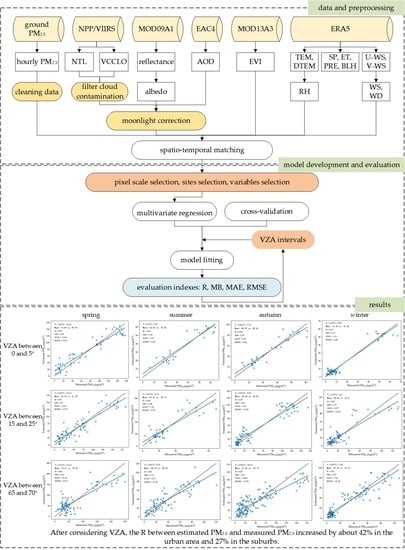
• It is essential to consider light anisotropy when utilizing NTL to estimate PM_2.5. In this study, coefficients between estimated PM_2.5 and measured PM_2.5 boosted greatly after introducing the satellite viewing zenith angle. Specifically, in four seasons it increased from 0.62, 0.56, 0.7, and 0.59 to 0.85, 0.89, 0.9, and 0.84 in the urban area, and from 0.54, 0.55, 0.64, and 0.59 to 0.71, 0.73, 0.8, and 0.7 in the suburbs.

References

1. Silver, B.; Reddington, C.; Arnold, S.; Spracklen, D. Substantial changes in air pollution across China during 2015–2017. Environ. Res. Lett. 2018, 13, 114012. [Google Scholar] [CrossRef]
2. Reddy, V.; Yedavalli, P.; Mohanty, S.; Nakhat, U. Deep air: Forecasting air pollution in Beijing, China. Environ. Sci. 2018. [Google Scholar]
3. Linares, C.; Diaz, J. Impact of particulate matter with diameter of less than 2.5 microns [PM2. 5] on daily hospital admissions in 0-10-year-olds in Madrid. Spain [2003–2005]. Gac. Sanit. 2009, 23, 192–197. [Google Scholar] [CrossRef] [PubMed]
4. Hansen, J.; Sato, M.; Ruedy, R. Radiative forcing and climate response. J. Geophys. Res. Atmos. 1997, 102, 6831–6864. [Google Scholar] [CrossRef]
5. Pui, D.Y.; Chen, S.-C.; Zuo, Z. PM2.5 in China: Measurements, sources, visibility and health effects, and mitigation. Particuology 2014, 13, 1–26. [Google Scholar] [CrossRef]
6. Cohen, A.J.; Brauer, M.; Burnett, R.; Anderson, H.R.; Frostad, J.; Estep, K.; Balakrishnan, K.; Brunekreef, B.; Dandona, L.; Dandona, R. Estimates and 25-year trends of the global burden of disease attributable to ambient air pollution: An analysis of data from the Global Burden of Diseases Study 2015. Lancet 2017, 389, 1907–1918. [Google Scholar] [CrossRef] [Green Version]
7. Hu, F.; Guo, Y. Health impacts of air pollution in China. Front. Environ. Sci. Eng. 2021, 15, 1–18. [Google Scholar] [CrossRef]
8. Li, J.; Carlson, B.E.; Lacis, A.A. How well do satellite AOD observations represent the spatial and temporal variability of PM2. 5 concentration for the United States? Atmos. Environ. 2015, 102, 260–273. [Google Scholar] [CrossRef]
9. Marsha, A.; Larkin, N.K. A statistical model for predicting PM2.5 for the western United States. J. Air Waste Manag. Assoc. 2019, 69, 1215–1229. [Google Scholar] [CrossRef]
10. Zhai, S.; Jacob, D.J.; Wang, X.; Shen, L.; Li, K.; Zhang, Y.; Gui, K.; Zhao, T.; Liao, H. Fine particulate matter (PM2.5) trends in China, 2013–2018: Separating contributions from anthropogenic emissions and meteorology. Atmos. Chem. Phys. 2019, 19, 11031–11041. [Google Scholar] [CrossRef] [Green Version]
11. You, W.; Zang, Z.; Zhang, L.; Li, Y.; Wang, W. Estimating national-scale ground-level PM2.5 concentration in China using geographically weighted regression based on MODIS and MISR AOD. Environ. Sci. Pollut. Res. 2016, 23, 8327–8338. [Google Scholar] [CrossRef] [PubMed]
12. Zou, B.; Chen, J.; Zhai, L.; Fang, X.; Zheng, Z. Satellite based mapping of ground PM2.5 concentration using generalized additive modeling. Remote Sens. 2017, 9, 1. [Google Scholar] [CrossRef] [Green Version]
13. Zhang, X.; Hu, H. Improving satellite-driven PM2.5 models with VIIRS nighttime light data in the Beijing–Tianjin–Hebei region, China. Remote Sens. 2017, 9, 908. [Google Scholar] [CrossRef] [Green Version]
14. Unnithan, S.K.; Gnanappazham, L. Spatiotemporal mixed effects modeling for the estimation of PM2.5 from MODIS AOD over the Indian subcontinent. GIScience Remote Sens. 2020, 57, 159–173. [Google Scholar] [CrossRef]
15. Wu, J.; Yao, F.; Li, W.; Si, M. VIIRS-based remote sensing estimation of ground-level PM2.5 concentrations in Beijing–Tianjin–Hebei: A spatiotemporal statistical model. Remote Sens. Environ. 2016, 184, 316–328. [Google Scholar] [CrossRef]
16. Geng, G.; Zhang, Q.; Martin, R.V.; van Donkelaar, A.; Huo, H.; Che, H.; Lin, J.; He, K. Estimating long-term PM2.5 concentrations in China using satellite-based aerosol optical depth and a chemical transport model. Remote Sens. Environ. 2015, 166, 262–270. [Google Scholar] [CrossRef]
17. Goldberg, D.L.; Gupta, P.; Wang, K.; Jena, C.; Zhang, Y.; Lu, Z.; Streets, D.G. Using gap-filled MAIAC AOD and WRF-Chem to estimate daily PM2.5 concentrations at 1 km resolution in the Eastern United States. Atmos. Environ. 2019, 199, 443–452. [Google Scholar] [CrossRef]
18. Wei, J.; Huang, W.; Li, Z.; Xue, W.; Peng, Y.; Sun, L.; Cribb, M. Estimating 1-km-resolution PM2.5 concentrations across China using the space-time random forest approach. Remote Sens. Environ. 2019, 231, 111221. [Google Scholar] [CrossRef]
19. Just, A.C.; Arfer, K.B.; Rush, J.; Dorman, M.; Shtein, A.; Lyapustin, A.; Kloog, I. Advancing methodologies for applying machine learning and evaluating spatiotemporal models of fine particulate matter (PM2.5) using satellite data over large regions. Atmos. Environ. 2020, 239, 117649. [Google Scholar] [CrossRef]
20. Yang, N.; Shi, H.; Tang, H.; Yang, X. Geographical and temporal encoding for improving the estimation of PM2.5 concentrations in China using end-to-end gradient boosting. Remote Sens. Environ. 2022, 269, 112828. [Google Scholar] [CrossRef]
21. Zeng, Q.; Xie, T.; Zhu, S.; Fan, M.; Chen, L.; Tian, Y. Estimating the Near-Ground PM2.5 Concentration over China Based on the CapsNet Model during 2018–2020. Remote Sens. 2022, 14, 623. [Google Scholar] [CrossRef]
22. Li, R.; Liu, X.; Li, X. Estimation of the PM2.5 pollution levels in Beijing based on nighttime light data from the defense meteorological satellite program-operational linescan system. Atmosphere 2015, 6, 607–622. [Google Scholar] [CrossRef] [Green Version]
23. Wang, J.; Aegerter, C.; Xu, X.; Szykman, J.J. Potential application of VIIRS Day/Night Band for monitoring nighttime surface PM2.5 air quality from space. Atmos. Environ. 2016, 124, 55–63. [Google Scholar] [CrossRef] [Green Version]
24. Zhao, X.; Shi, H.; Yu, H.; Yang, P. Inversion of nighttime PM2.5 mass concentration in Beijing based on the VIIRS day-night band. Atmosphere 2016, 7, 136. [Google Scholar] [CrossRef] [Green Version]
25. Zhao, X.; Shi, H.; Yang, P.; Zhang, L.; Fang, X.; Liang, K. Inversion algorithm of PM2.5 air quality based on nighttime light data from NPP-VIIRS. J. Remote Sens. 2017, 21, 291–299. [Google Scholar]
26. Ke, L.; Chaoshun, L.; Penglong, J. Estimation of nighttime PM2.5 concentration in Shanghai based on NPP/VIIRS Day Night Band data. Acta Sci. Circumstantiae 2019, 39, 1913–1922. [Google Scholar]
27. Fu, D.; Xia, X.; Duan, M.; Zhang, X.; Li, X.; Wang, J.; Liu, J. Mapping nighttime PM2.5 from VIIRS DNB using a linear mixed-effect model. Atmos. Environ. 2018, 178, 214–222. [Google Scholar] [CrossRef]
28. Wang, M.; Wang, Y.; Teng, F.; Li, S.; Lin, Y.; Cai, H. Estimation and Analysis of PM2.5 Concentrations with NPP-VIIRS Nighttime Light Images: A Case Study in the Chang-Zhu-Tan Urban Agglomeration of China. Int. J. Environ. Res. Public Health 2022, 19, 4306. [Google Scholar] [CrossRef]
29. Chen, H.; Xu, Y.; Mo, Y.; Zhang, Y.; Yang, Z. Estimating nighttime PM2.5 concentrations in Huai’an based on NPP/VIIRS nighttime light data. Acta Sci. Circumstantiae 2022, 42. [Google Scholar]
30. Li, X.; Zhang, C.; Li, W.; Liu, K. Evaluating the use of DMSP/OLS nighttime light imagery in predicting PM2.5 concentrations in the northeastern United States. Remote Sens. 2017, 9, 620. [Google Scholar] [CrossRef] [Green Version]
31. McHardy, T.; Zhang, J.; Reid, J.; Miller, S.; Hyer, E.; Kuehn, R. An improved method for retrieving nighttime aerosol optical thickness from the VIIRS Day/Night Band. Atmos. Meas. Tech. 2015, 8, 4773–4783. [Google Scholar] [CrossRef] [Green Version]
32. Zhang, G.; Shi, Y.; Xu, M. Evaluation of LJ1-01 nighttime light imagery for estimating monthly PM2.5 concentration: A comparison with NPP-VIIRS nighttime light data. IEEE J. Sel. Top. Appl. Earth Obs. Remote Sens. 2020, 13, 3618–3632. [Google Scholar] [CrossRef]
33. Johnson, R.S.; Zhang, J.; Hyer, E.J.; Miller, S.D.; Reid, J.S. Preliminary investigations toward nighttime aerosol optical depth retrievals from the VIIRS Day/Night Band. Atmos. Meas. Tech. 2013, 6, 1245–1255. [Google Scholar] [CrossRef] [Green Version]
34. Román, M.O.; Wang, Z.; Sun, Q.; Kalb, V.; Miller, S.D.; Molthan, A.; Schultz, L.; Bell, J.; Stokes, E.C.; Pandey, B. NASA’s Black Marble nighttime lights product suite. Remote Sens. Environ. 2018, 210, 113–143. [Google Scholar] [CrossRef]
35. Kyba, C.C.; Aubé, M.; Bará, S.; Bertolo, A.; Bouroussis, C.A.; Cavazzani, S.; Espey, B.R.; Falchi, F.; Gyuk, G.; Jechow, A. Multiple angle observations would benefit visible band remote sensing using night lights. J. Geophys. Res. Atmos. 2022, 127, e2021JD036382. [Google Scholar] [CrossRef]
36. Lee, S.; Chiang, K.; Xiong, X.; Sun, C.; Anderson, S. The S-NPP VIIRS day-night band on-orbit calibration/characterization and current state of SDR products. Remote Sens. 2014, 6, 12427–12446. [Google Scholar] [CrossRef] [Green Version]
37. Deng, Y.; Liu, J.; Liu, Y.; Xu, S. Spatial distribution estimation of PM2.5 concentration in Beijing by applying Bayesian geographic weighted regression model. Sci. Surv. Mapp. 2018, 43, 39–45. [Google Scholar]
38. Rohde, R.A.; Muller, R.A. Air pollution in China: Mapping of concentrations and sources. PLoS ONE 2015, 10, e0135749. [Google Scholar] [CrossRef]
39. Liao, L.; Weiss, S.; Mills, S.; Hauss, B. Suomi NPP VIIRS day-night band on-orbit performance. J. Geophys. Res. Atmos. 2013, 118, 12705–712718. [Google Scholar] [CrossRef]
40. Qiu, S.; Shao, X.; Cao, C.Y.; Uprety, S.; Wang, W.H. Assessment of straylight correction performance for the VIIRS Day/Night Band using Dome-C and Greenland under lunar illumination. Int. J. Remote Sens. 2017, 38, 5880–5898. [Google Scholar] [CrossRef]
41. Baker, N. Joint Polar Satellite System (JPSS) VIIRS Cloud Cover/Layers Algorithm Theoretical Basis Document (ATBD). NASA Goddard Space Flight Cent. Tech. Rep. 2011. [Google Scholar]
42. Liang, W.G.; Zhao, Y.S. A new method of surface albedo inverse model based on energy transmission. Remote Sens. Land Resour. 2007, 19, 53–56. [Google Scholar]
43. Miller, S.D.; Turner, R.E. A Dynamic Lunar Spectral Irradiance Data Set for NPOESS/VIIRS Day/Night Band Nighttime Environmental Applications. IEEE Trans. Geosci. Remote Sens. 2009, 47, 2316–2329. [Google Scholar] [CrossRef]
44. Li, X.; Ma, R.; Zhang, Q.; Li, D.; Liu, S.; He, T.; Zhao, L. Anisotropic characteristic of artificial light at night – Systematic investigation with VIIRS DNB multi-temporal observations. Remote Sens. Environ. 2019, 233, 111357. [Google Scholar] [CrossRef]
45. Kocifaj, M.; Bará, S. Aerosol characterization using satellite remote sensing of light pollution sources at night. Mon. Not. R. Astron. Soc. Lett. 2020, 495, L76–L80. [Google Scholar] [CrossRef] [Green Version]
46. Kocifaj, M.; Bará, S. Diffuse light around cities: New perspectives in satellite remote sensing of nighttime aerosols. Atmos. Res. 2022, 266, 105969. [Google Scholar] [CrossRef]
Figure 1. The distribution of PM2.5 monitoring sites in Beijing, which is divided into urban and suburban areas and contains four types of monitoring sites.
Remotesensing 15 00349 g001
Figure 2. Images of VIIRS for Beijing: (a,b) DNB radiance at 17:44 on 3 January 2019 and 17:36 on 13 December 2018, respectively; solid circles denote 34 PM2.5 monitoring sites. For (a), the VZA, LZA, and daily PM2.5 were 34.33°, 133.77°, and 18 μg/m3, respectively; the set of these data for (b) were (41.45°, 128.16°, 48 μg/m3). (c,d) The VCCLO corresponding to (a,b).
Remotesensing 15 00349 g002
Figure 3. Scatter plots of PM2.5/μ and ln(I): (a) is the DS site while (b) is the FS site; Imean is the annual mean of radiance. The dashed line is the fit curve.
Remotesensing 15 00349 g003
Figure 4. Inter-comparison between hourly mean PM2.5 (y-axis) measured at overpass time of NPP (2:00 CST) and Terra (11:00 CST) and daily PM2.5 (x-axis): (ad) is in spring, summer, autumn, and winter, respectively. The dashed line is the 1:1 line as a reference.
Remotesensing 15 00349 g004
Figure 5. Histograms of variables in this study: (a) PM2.5; (b) radiance; (c) relative humidity; (d) surface pressure; (e) evaporation; (f) precipitation; (g) wind speed; (h) wind direction; (i) boundary layer height; (j) temperature; (k) EVI.
Remotesensing 15 00349 g005aRemotesensing 15 00349 g005b
Figure 6. Scatter plots of estimated PM2.5 and measured PM2.5 without considering VZA in the urban area and the suburbs: (ad) is in spring, summer, autumn, and winter of the urban area, respectively; (eh) is the same in the suburbs. The dashed line is the 1:1 line as a reference.
Remotesensing 15 00349 g006
Figure 7. Scatter plots of estimated PM2.5 and measured PM2.5 at subsatellite points in the urban area and the suburbs: (ad) is in spring, summer, autumn, and winter of the urban area, respectively; (eh) is the same in the suburbs. The dashed line is the 1:1 line as a reference.
Remotesensing 15 00349 g007aRemotesensing 15 00349 g007b
Figure 8. The boxplot of R of estimated PM2.5 and measured PM2.5. Marker ‘+’ represents the mean of R, and diamond ‘◆’ represents the outlier below the lower boundary line.
Remotesensing 15 00349 g008
Figure 9. Comparison of measured PM2.5 and estimated PM2.5 based on VIIRS/DNB data in the sequences of validation set: (a) is in the urban area. (b) is in the suburbs.
Remotesensing 15 00349 g009aRemotesensing 15 00349 g009b