Assessment of Dynamic Mode Decomposition (DMD) Model for Ionospheric TEC Map Predictions

Abstract

In this study, we assess the Dynamic Mode Decomposition (DMD) model applied with global ionospheric vertical Total Electron Content (vTEC) maps to construct 24-h global ionospheric vTEC map forecasts using the available International GNSS Service (IGS) 2-h cadence vTEC maps. In addition, we examine the impact of a EUV 121.6 nm time series data source with the DMD control (DMDc) framework, which shows an improvement in the vTEC Root Mean Square Error (RMSE) values compared with the IGS final solution vTEC maps. Both the DMD and DMDc predictions present close RMSE scores compared with the available CODE 1-day predicted ionospheric maps, both for quiet and disturbed solar activity. Finally, we evaluate the predicted global ionospheric vTEC maps with the East-North-Up (ENU) coordinate system errors metric, as an ionospheric correction source for L1 single-frequency GPS/GNSS Single Point Positioning (SPP) solutions. Based on these findings, we argue that the commonly adopted vTEC map comparison RMSE metric fails to correctly reflect an informative impact with L1 single-frequency positioning solutions using dual-frequency ionospheric corrections.

1. Introduction

The ionization processes in the ionosphere, Earth’s upper atmosphere layer which ranges between 60 km to 1000 km, are mainly driven by X-ray and Extreme Ultra Violet (EUV) solar irradiance which ionizes the air molecules and consequently creates a layer of free electrons [1,2,3,4,5,6]. The ionosphere layer has a significant impact on radio waves communication and navigation propagating through it [7,8,9]. For example, small-scale ionospheric irregularities can scatter radio waves and generate rapid fluctuations (or scintillation) in the amplitude and phase of Global Navigation Satellite Systems (GNSS) received signals, leading to cycle slips that degrade the receiver’s ability to hold a lock on a signal [10,11,12,13].

The Total Electron Content (TEC) amount produced in the ionosphere is measured in TEC units (1 TECU = ${10}^{16}\mathrm{electrons}/{\mathrm{m}}^2$) and refers to the total count of integrated electrons along the ionosphere vertically crossing a 1${\mathrm{m}}^2$ base cylinder [14,15,16]. It is the main parameter which is used in space weather research to quantify the amount of ionospheric disturbance and commonly represented as a global vertical TEC (vTEC) map with $2.5^{\circ }$, $5^{\circ }$ (degree) latitude, longitude resolution, respectively [17,18]. Thus, acquiring the ability to accurately forecast and estimate future TEC values at a global scale can enhance the accuracy of space-borne as well as increase their quality and reliability by compensating for data loss probabilities and delays.

Since 1998, the International GNSS Service (IGS) has provided global ionosphere vTEC maps derived from dual-frequency GNSS data, using more than 380 IGS stations with approximately 11 days latency for the final vTEC maps solution [19,20]. Its associated agency, the Center for Orbit Determination in Europe (CODE), provides rapid global TEC maps with a temporal resolution of 2 h and a latency below 24 h [21,22]. Similarly, The Jet Propulsion Laboratory (JPL), jointly with The University of Southern California (USC), has developed the Global Assimilative Ionospheric Model (GAIM), which numerically solves for ion and electron volume densities through the hydrodynamic equations for individual ions, and is represented as a global TEC map [23]. In parallel and jointly with the IGS, the European Space Agency/European Space Operations Center (ESA/ESOC) also contributes IONEX products to the IGS ionosphere Working Group. More recently, the Chinese Academy of Sciences (CAS), started generating GIM products using a two-step Spherical Harmonic function Plus generalized Trigonometric Series (SHPTS) approach. In addition, the Canadian Geodetic Survey of Natural Resources Canada (NRCAN) generates daily global maps using GNSS phase-smoothed geometry-free pseudorange measurements with a single-layer model from approximately 350 stations, thus their products also contribute to the IGS products. Roma-Dollase et al. [24] a comprehensive comparison of the performances between all the GIMs created in the frame of IGS.

The availability and historical records of these data sources, along with the advancement of Machine Learning (ML) and Deep Learning (DL) algorithms and hardware development of graphical processing units (GPUs) in the past decade, has led to near human-level performance in different scientific fields, such as computer vision, natural language processing, robotics, and gaming [25], which in turn has attracted the attention of the big data and ML scientific community for pursuing more accurate forecasts while exploring various ML methods.

In the field of Space Weather, AI is utilized in various scenarios ranging from predictions of the probability for solar flares occurrence, originated on the Sun’s surface [17,18,26], to creating global TEC models using gradient boosting, a machine-learning-based technique [27]. Liu et al. [28] applied with a long short-term memory (LSTM) neural network (NN) with multiple input data, including historical time series of spherical harmonics (SH) coefficients, solar extreme ultraviolet (EUV) flux, disturbance storm time (Dst), and hour of the day indices to forecast the 256 SH coefficients which are used in global ionospheric maps (GIMs) construction. The results were comprehensively evaluated with respect to the CODE GIM vTEC estimations. Later on, Lee et al. [29] proposed a DL method based on conditional generative adversarial networks (cGAN) for forecasting global TEC maps using a one-day candidate. The model was trained with IGS TEC maps and the results were compared with the CODE-predicted maps.

Recently, Tang et al. [30] proposed an ionospheric TEC forecasting using neural network (NN), consisting of a convolutional neural network (CNN), long-short term memory (LSTM) neural network combined with an attention mechanism. The model was fed with TEC time series, Bz, Kp, Dst, and F10.7 parameters from 24 GNSS stations, and the results were compared to NeQuick, LSTM, and CNN-LSTM forecast models, examining the RMSE and TECU scores. A similar approach was proposed by Liu et al. [31], who applied convolutional long short-term memory (convLSTM)-based machine learning models to forecast global ionospheric total electron content (TEC) maps with up to 24 h of lead time at a 1-h interval. While Xia et al. [32] proposed the conv-attentional image time sequence transformer (CAiTST), a transformer-based image time sequences prediction model equipped with convolutional networks and an attentional mechanism. The model was trained with IGS TECU maps between the years 2005 to 2017 and compared to the 1-day CODE prediction model using RMSEs score. In addition, a three-step TEC modeling method, based on the machine learning approach, was proposed by Liu et al. [33] to establish an empirical prediction model of TEC over parts of Europe. The model is based on principal component analysis (PCA), solar activity parameters—F10.7, and the sunspot number (R12) parameter, while using modified Kriging spatial interpolation. The method uses regression learning for determining the coefficients and harmonic numbers of the model by using RMSE values. As a final step, the model results are compared to the IRI model.

In this study, we introduce Dynamic Mode Decomposition (DMD) as a technique to forecast one-day GIM with a two-hour candidate. In addition, we expand our study by introducing EUV time series data as an external input to the DMD, by utilizing the DMD with Control (DMDc) framework [34], to examine its ability for forecasting, as well as estimating the contribution of EUV under the chosen model. We assess our results with ten representative case studies during solar flare days and ten representative case studies during quiet solar activity days. In addition, we also examine nine Coronal Mass Ejection (CME) storm-featured days. The results are analyzed in terms of Root Mean Square Error (RMSE), compared between the DMD/DMDc/CODE-predicted GIMs, as well as the East-North-Up (ENU) error positions, calculated using the “gLab” software [35] with the predicted GIMs maps as a single frequency (L1 = 1575.42 MHz) positioning correction input.

2. Methodology

The DMD is a data-driven approach which was developed initially by the fluids dynamics community [36] to identify spatial and temporal coherent structures from high-dimensional data. It is based on Proper Orthogonal Decomposition (POD) and utilizes the efficiency of Singular Value Decomposition (SVD) [37,38]; however, unlike to SVD and POD, the DMD provides mode decomposition, where each mode has the same linear behavior of spatially correlated structures in time. From a data science perspective, the DMD is an algorithm that identifies the best-fit linear dynamical system which advances high dimensional measurements forward in time. Since it was first introduced, it has gained popularity in the field of fluid dynamics [39,40,41,42] as a tool for analyzing nonlinear dynamical systems data, primarily arranged sequentially as time series snapshots of the system, hence, it shares spatial and temporal distribution similarities with the TEC GIMs.

The DMD approach requires a data set matrix consisting of column vectors which represent the system’s snapshots as they spatiotemporally evolve [43]. We denote this data set of m snapshots by ${\left\{x_t\right\}}_{t=1}^m$ where $x_t$ constitutes a system state sampled at discrete time t that is reshaped into a high-dimensional column vector. The number of system snapshots m is considered as a parameter that defines the number of snapshots (system history) and the maximum number of dynamic modes. In turn, the data set is split into two matrices, X and $X^{\prime }$, such that:

$$X=\left[\begin{array}{cccc}|& |& |& |\\ x_1& x_2& \dots & x_{m-1}\\ |& |& |& |\end{array}\right]$$

(1)

$$X^{\prime }=\left[\begin{array}{cccc}|& |& |& |\\ x_2& x_3& \dots & x_m\\ |& |& |& |\end{array}\right]$$

(2)

The DMD algorithm aims to establish the best-fit linear transformation A which transforms the system snapshots from matrix X to matrix $X^{\prime }$, thus finding the best linear approximation for the dynamical system that temporally transforms between the two matrices:

$$X^{\prime }\approx AX$$

(3)

If the snapshots $x_t$ is sampled with constant $\Delta t$, such that $x_{t+1}=x_{t+\Delta t}$, then:

$$x_{t+1}\approx A{x}_t$$

(4)

Formally, the best-fit transformation matrix A is defined as:

$$A=\underset{A}{arg\; min}\left|\right|X^{\prime }-AX{\left|\right|}_F=X^{\prime }{X}^{†}$$

(5)

where $\left|\right|·{\left|\right|}_F$ is the Frobenius norm and ${}^{†}$ is the pseudo-inverse. The efficiency of the DMD algorithm emerges from leveraging dimensionality reduction for computing the eigenvalues and eigenvectors of matrix A without requiring any explicit computations using it directly. If $x\in {\mathbb{R}}^n$ is a high-dimensional snapshot column vector, then matrix A consists of $n^2$ elements, which can make its representation, as well as its eigendecomposition, complex and unmanageable. Instead, the singular value decomposition of matrix X is used to compute the pseudo-inverse $X^{†}$. In general, matrix X has fewer columns (m) than rows (n), meaning $m\ll n$, which results at most in m non-zero singular values of the eigendecomposition, thus the matrix A has at most rank m. As such, A can be projected onto the leading singular vectors of the decomposition, resulting in a smaller matrix $\tilde{A}$ with at most m x m dimensions. In addition, one can choose to utilize SVD truncation parameter r in order to truncate singular vectors that correspond to small non-zero singular values, in that case, the truncated SVD only approximates X. A principled hard-thresholding algorithm proposed by Gavish and Donoho [44], to optimally determine parameter r from noisy data.

2.1. Dynamic Mode Decomposition

The algorithmic steps of the DMD provided by Tu [45] are as follows:

1.

Computing the truncated singular value decomposition of X

$$X\approx \tilde{U}\tilde{\Sigma }{\tilde{V}}^{*}$$

(6)

where $\tilde{U}\in {\mathbb{C}}^{nxr}$,$\tilde{\Sigma }\in {\mathbb{C}}^{rxr}$ and $\tilde{V}\in {\mathbb{C}}^{mxr}$. The ${}^{*}$ denotes the complex conjugate and $r\le m$ denotes the truncation parameter, therefore, constitutes the exact or approximation rank of matrix X. Note that, $\tilde{U}$ and $\tilde{V}$ are both semi-unitary matrix, such that ${\tilde{U}}^{*}\tilde{U}={\tilde{V}}^{*}\tilde{V}=I$, while $\tilde{U}$ are also know as the POD modes.

2.

Projecting A onto the POD modes in $\tilde{U}$ to yield the compact representation $\tilde{A}$ which captures the leading r nonzero eigenvalues and eigenvectors of A. Recall from Equation (6) the pseudo-inverse of X:

$$X^{†}\approx \tilde{V}{\tilde{\Sigma }}^{-1}{\tilde{U}}^{*}$$

(7)

Therefore, following Equation (5)

$$\tilde{A}={\tilde{U}}^{*}A\tilde{U}={\tilde{U}}^{*}{X}^{\prime }\tilde{V}{\tilde{\Sigma }}^{-1}{\tilde{U}}^{*}\tilde{U}={\tilde{U}}^{*}{X}^{\prime }\tilde{V}{\tilde{\Sigma }}^{-1}$$

(8)

The compact representation $\tilde{A}$ encapsulate the linear dynamics of the system for POD vector $\tilde{x}$, such that

$${\tilde{x}}_{t+1}=\tilde{A}\tilde{x}$$

(9)

whereas the matrix $\tilde{U}$ constitute the transformation between the full system state x and the POD state $\tilde{x}$, that is $x=\tilde{U}\tilde{x}$.

One can acquire the DMD modes of the high-dimensional matrix A, by following a few additional steps:

3.

Computing the eigendecomposition of $\tilde{A}$:

$$\tilde{A}W=W\Lambda$$

(10)

The diagonal values of $\Lambda$ matrix correspond to the eigenvalues of matrix A which is also the DMD eigenvalues. While the columns of matrix W are the eigenvectors of $\tilde{A}$ and are considered as a linear combination of POD mode amplitudes.

4.

Finally, constructing the high-dimensional DMD modes $\Phi$ by utilizing previously computed eigenvectors in W of the snapshot matrix $X^{\prime }$.

$$\Phi =X^{\prime }\tilde{V}{\tilde{\Sigma }}^{-1}W$$

(11)

In fact, the DMD modes are the eigenvectors of matrix A corresponding to the eigenvalues of $\Lambda$.

$$A\Phi =(X^{\prime }\tilde{V}{\tilde{\Sigma }}^{-1}\underset{\tilde{A}}{\underbrace{{\tilde{U}}^{*}\left)\right(X^{\prime }\tilde{V}{\tilde{\Sigma }}^{-1}}}W)=X^{\prime }\tilde{V}{\tilde{\Sigma }}^{-1}\tilde{A}W=X^{\prime }\tilde{V}{\tilde{\Sigma }}^{-1}W\Lambda =\Phi \Lambda$$

(12)

2.2. Dynamic Mode Decomposition with Control (DMDc)

The DMDc was first introduced by Proctor et al. [34], as an extension to the DMD in order to incorporate the effect of control, for extracting low-order models from high-dimensional complex systems, where external forcing has been applied during the observation period. The goal of the DMDc is to establish the relationship in a dynamical system between the future state $x_{t+1}$ with the current state $x_t$ measurement and the current input signal $u_t$ measurement, given by the following linear expression:

$$x_{t+1}=A{x}_t+B{u}_t$$

(13)

where $x_t\in {\mathbb{R}}^n$, $u_t\in {\mathbb{R}}^q$, $A\in {\mathbb{R}}^{nxn}$ and $B\in {\mathbb{R}}^{nxq}$. Similar to DMD, the operator A constitutes the temporal and spatial transition dynamics of the unforced system, while the operator B describes the impact of the input signal $u_t$ with the future state. As for the DMD, the DMDc seeks to find an approximation of A and B from the recorded measurements, this means that the equality in the term presented in Equation (13) does not have to be exactly satisfied. The DMDc utilizes the same snapshot matrices $X^{\prime }$ and X as DMD, but with an addition of the input measurement matrix ${\rm Y}$:

$${\rm Y}=\left[\begin{array}{cccc}|& |& |& |\\ u_1& u_2& \dots & u_{m-1}\\ |& |& |& |\end{array}\right]$$

(14)

Equation (13) can be rewritten as:

$$X^{\prime }=AX+B{\rm Y}$$

(15)

In [34] study, two cases for the DMDc were presented. The first one is where the control matrix B is known, while the second is where it was unknown. We will present the second scenario, as it is the case in our study, i.e., finding the approximation of operators A and B exclusively from snapshot data. The system described in Equation (15) can be rearranged as:

$$X^{\prime }=\left[\begin{array}{cc}A& B\end{array}\right]\left[\begin{array}{c}X\\ {\rm Y}\end{array}\right]=G\Omega$$

(16)

where G and $\Omega$ are the augmented operators of $\left[\begin{array}{cc}A& B\end{array}\right]$ and $\left[\begin{array}{c}X\\ {\rm Y}\end{array}\right]$, respectively. The DMDc constitutes the eigendecomposition of the operator A defined by

$$G=X^{\prime }{\Omega }^{†}$$

(17)

$$\left[\begin{array}{cc}A& B\end{array}\right]=X^{\prime }{\left[\begin{array}{c}X\\ {\rm Y}\end{array}\right]}^{†}$$

(18)

where $\Omega$ contains the vertically appended control snapshot ${\rm Y}$ with the system snapshots X. As with the DMD, an SVD is utilized with $\Omega$, such that $\Omega =\tilde{U}\tilde{\Sigma }{\tilde{V}}^{*}$ with truncation parameter $\tilde{r}$, to find a solution which minimizes the Frobenius norm of $\left|\right|X^{\prime }-G\Omega {\left|\right|}_F$ and solve for G or its approximate $\overline{G}$.

$$G\approx \overline{G}=X^{\prime }\tilde{V}{\tilde{\Sigma }}^{-1}{\tilde{U}}^{*}$$

(19)

where $G\in {\mathbb{R}}^{nx(n+q)}$, therefore an approximation for A and B can be found by splitting matrix $\tilde{U}$:

$$\left[\begin{array}{cc}A& B\end{array}\right]=\left[\begin{array}{cc}{X}^{\prime }\tilde{V}{\tilde{\Sigma }}^{-1}{\tilde{U}}_1^{*}& X^{\prime }\tilde{V}{\tilde{\Sigma }}^{-1}{\tilde{U}}_2^{*}\end{array}\right]$$

(20)

where ${\tilde{U}}_1\in {\mathbb{R}}^{nxr}$, ${\tilde{U}}_2\in {\mathbb{R}}^{qxr}$ and ${\tilde{U}}^{*}=\left[\begin{array}{cc}{\tilde{U}}_1^{*}& {\tilde{U}}_2^{*}\end{array}\right]$. We note that the DMD uses the POD matrix $\tilde{U}$ in order to transform the high-dimensional state into a reduced-order approximation subspace. With the DMDc the case is different since $\tilde{U}$ is defined for the input space, consisting of the system measurements and the signal inputs, in order to form a low-rank model of the dynamics DMDc utilizes the $X^{\prime }$ matrix. Therefore, an additional SVD is applied on $X^{\prime }$ with a truncation parameter r, such that $X^{\prime }=\widehat{U}\widehat{\Sigma }{\widehat{V}}^{*}$, where $\widehat{U}\in {\mathbb{R}}^{nxr}$, $\widehat{\Sigma }\in {\mathbb{R}}^{rxr}$, and $\widehat{V}\in {\mathbb{R}}^{rxm-1}$. Then, the reduced-order approximation of A and B is computed utilizing the transformation $x=\widehat{U}\tilde{x}$:

$$\tilde{A}={\widehat{U}}^{*}\overline{A}\widehat{U}={\widehat{U}}^{*}{X}^{\prime }\tilde{V}{\tilde{\Sigma }}^{-1}{\tilde{U}}_1^{*}\widehat{U}$$

(21)

$$\tilde{B}={\widehat{U}}^{*}\overline{B}={\widehat{U}}^{*}{X}^{\prime }\tilde{V}{\tilde{\Sigma }}^{-1}{\tilde{U}}_2^{*}$$

(22)

where $\tilde{A}\in {\mathbb{R}}^{rxr}$ and $\tilde{B}\in {\mathbb{R}}^{rxl}$, from Equations (21) and (22) the reduced-order model can be constructed as:

$${\tilde{x}}_{t+1}=\tilde{A}{\tilde{x}}_t+\tilde{B}{u}_t$$

(23)

Similar to the DMD, by solving the eigenvalue decomposition of $\tilde{A}W=W\Lambda$ and transforming from the eigenvector by the following formula:

$$\varphi =X^{\prime }\tilde{V}{\tilde{\Sigma }}^{-1}{\tilde{U}}_1^{*}\widehat{U}w$$

(24)

we acquire the dynamic modes of A.

3. Data and Forecast

Following previous studies, which consider the 2-h IGS final solution candidate GIMs as a suitable data reference for ML training, we also utilized the IGS 2-h candidate data source for constructing a DMD and DMDc suitable data set. In addition, we used the publicly available 24-h predicted GIMs provided by the CODE analysis center for comparison purposes. Suitable IGS and CODE GIMs data range were selected to cover peak activity during solar cycle 24, specifically between the beginning of 2013 and the end of 2014, and an additional nine CME storm events between 2015, 2017, 2018, and 2019.

Table 1. Case studies table, containing all the dates for the quiet, disturbance, and CME event, along with their corresponding X-ray magnitudes and Kp indices.

Study Case Events
Quiet Events	Magnitude	Disturbance Events	Magnitude	CME Date	Kp Max
23/08/2014	C6.0	25/02/2014	X4.9	17/03/2015	8−
25/01/2014	C1.0	24/10/2014	X3.1	22/06/2015	8+
15/02/2014	C2.3	10/06/2014	X2.2	23/06/2026	8−
26/03/2014	C1.5	27/10/2014	X2.0	08/09/2017	8+
09/04/2014	C2.1	26/10/2014	X2.0	28/09/2017	7−
29/05/2014	C1.4	20/12/2014	X1.8	25/08/2018	4+
23/06/2014	C1.0	07/11/2014	X1.6	26/08/2018	7+
22/07/2014	B2.8	22/10/2014	X1.6	20/08/2018	6
20/09/2014	C1.1	10/09/2014	X1.6	01/09/2019	5+
11/10/2014	C1.8	25/04/2014	X1.3	–/–/–	–

sums up all selected case studies for comparison.

IGS and CODE data are available at ftp://gdc.cddis.eosdis.nasa.gov (accessed on 23 December 2022) FTP server, until 2020, and at https://cddis.nasa.gov/ (accessed on 23 December 2022) with HTTPS/FTP-SSL access.The data sources achieve a daily IONEX file which consists of 13 GIMs at 2-h resolution time span (note, that the last (thirteen) GIM of each day is overlapping with the first GIM of the following day). Each GIM is represented in a matrix form, containing scaled vTEC values, with dimensions of $71\times 73$ which corresponds to $2.5^{\circ }$ latitude and $5^{\circ }$ longitude resolutions, respectively [20,46]. 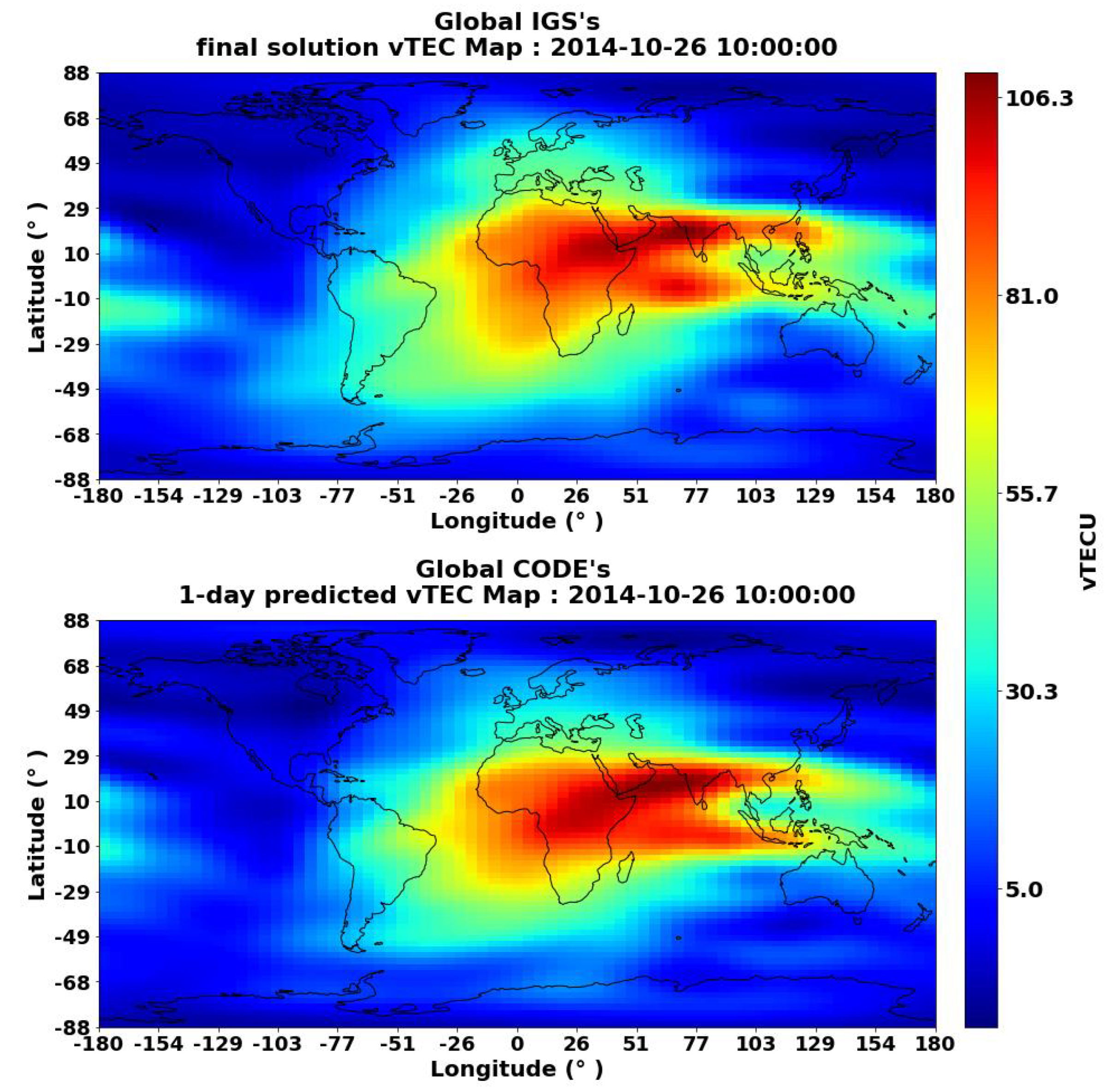Figure 1(top) shows an example of a typical vTEC map provided by IGS and Figure 1(bottom) shows an example of a predicted vTEC map provided by CODE analysis center.

In addition to GIMs data, we also utilized the available 1-min cadence 121.6 nm EUV yearly data, corresponding to the years 2013–2015 and 2017–2019. The EUV is provided by NOAA’s Geostationary Operational Environmental Satellites (GOES). The GOES-15 and GOES-16 missions are equipped with Extreme Ultraviolet Sensor (EUVS) instruments which measure the EUV in 5 channels ranging between 5 and 125 nm [47,48]. The EUV measurements data of GOES 15 and 16 are publicly available since 2010 with a 1-min cadence at https://satdat.ngdc.noaa.gov/sem/goes/data/euvs/netcdf/goes15 (accessed on 23 December 2022) and https://data.ngdc.noaa.gov/platforms/solar-space-observing-satellites/goes/goes16, respectively (accessed on 23 December 2022). Figure 2 illustrate the EUV irradiance data acquired from the GOES-15 mission during 2013–2014.

3.1. Preprocessing

In order to apply the DMD algorithm as a daily vTEC GIMs prediction mechanism, a suitable data set should be constructed and properly organized. The DMD requires a data set shaped in a matrix form, consisting of column vectors that constitute snapshots of a dynamical system evolving in time. We consider every vTEC GIM with a 2-h cadence as a system snapshot. Therefore, we select daily IGS IONEX files which cover an entire year of snapshots for every case study (Table 1), resulting in 365 daily IGS IONEX files for each year out of 2013, 2014, 2015, 2017, 2018, and 2019, respectively. Afterward, for every IONEX file, we drop the thirteenth GIM (as it overlaps with the first GIM of the following day file), and the remaining twelve GIMs are considered as system snapshots. In turn, each GIM snapshot is reshaped from a matrix form into a column vector and stacked together to form a daily matrix of snapshots with twelve columns. More formally, each original GIM with 71 × 73 shape is reshaped into a column vector with 5183 × 1 dimensions and stacked together to form a 5183 × 12 daily 2-h time span snapshots matrix. Finally, we stack all the daily snapshots matrices into one general data matrix, consisting of a 2-h cadence dynamical system of snapshots, formed entirely from the selected data range. Figure 3 illustrates an example of constructing a general data matrix and prepossessing for GIMs ranging between 2013 and 2014. The total number of days in the selected data range is 2190 (365 × 6) days, resulting in 5183 × 26,280 (26,280 = 2190 × 12) general data matrix dimensions.

Similar to the DMD approach, the DMDc also requires a data set matrix which consists of system snapshots, organized as vector columns along with the addition of control input signals. Each control input signal which corresponds to a particular snapshot is stacked vertically with the column vector of the snapshot (Equation (16)), constructing a column vector consisting of the system snapshot followed by the control input signal.

We select a suitable EUV 121.6 nm time series control input signal with two parameters: $length$—the control input signal length and $shift$—the amount of EUV data which will be ignored prior to the snapshot time. At first, we mark the initial time of the system snapshot (GIM epoch) as a zero shift location. The zero shift location constitutes a reference position for ignoring the $shift$ amount of EUV data backward prior to the snapshot time. Once the $shift$ amount of EUV data is skipped, the actual control input signal with length $length$ is selected backwardly prior to the ignored $shift$ amount. Figure 4 illustrates an example for selecting a control input signal for a particular snapshot from EUV 121.6 nm time series data. In addition, the control input signals, which are part of the pre-processing and general matrix construction, are normalized to zero mean and standard deviation equal to 1, before being stacked to the corresponding system snapshot vector.

3.2. GIMs Predictions

In order to apply the DMD algorithm and generate 24-h predictions of GIMs (i.e., daily predictions), we select a data set matrix out of the general data matrix with h snapshots prior to the target prediction GIM. We choose a data set matrix with $h=1440$ which constitutes 120 days of history, meaning that approximately 4 months of historical data are used in order to estimate the transition matrix A, Equation (3). Once a particular data set matrix is selected based on the target prediction day, we apply the DMD with that data set matrix, which yields a transition matrix A. In turn, we use the transition matrix A with the last snapshot (snapshot number 1440) out of the snapshots in the data set matrix in order to predict 24 future snapshots (GIMs) as described in Equation (9).

Using this procedure, we applied the DMD with data set matrices which correspond to the case studies in Table 1 and utilized the yielded transition matrices to perform predictions for the first 24 h with a 2-h candidate for each case study.

Similarly, we select the data set matrix with $h=1440$ parameter for the DMDc, while vertically stacking control input signals to matrix’s snapshots with particular control input parameters: $shift$ and $length$. Once the control input’s parameters are fixed and the control inputs are vertically stacked to a particular data set matrix, as described in Equation (16), we acquire the transition matrix A and B by applying the DMDc with that data set matrix. Then, we use matrices A and B and the last snapshot and control input from the data set matrix to predict the target GIM. Note that applying the DMDc as GIM forecasting approach assumes that the future EUV control input signal is available. This means that the continuity of GIMs prediction over the target GIM, as described in Equation (23), forces the use of a control input which corresponds to the previously predicted GIM which isn’t available. In addition, the control input signal should be normalized with the normalizing parameters acquired during control inputs stacking normalization.

This technique is applied to generate GIM predictions, subject to every case study with various control input parameters.

4. Results

Following the above mentioned methodology, we made a comprehensive evaluation of the predicted GIMs over 24 h with 2-h candidates for various scenarios. We evaluated ten case studies during disturbed solar activity days (manifested as strong solar flare activity due to the influence of extreme UV and X-ray radiation on the Ionospheric F2 layer), ten case studies during quiet solar activity days, and an additional nine case studies characterized by CME storms. Table 1 contains the full case studies description.

As a first step, we applied the DMD with a relevant data set matrix for each case study and performed a prediction for 24 h with 2-h candidate. We evaluated the predicted GIMs vTEC with the RMSE metric compare to IGS final solution estimations. In addition, we also evaluated our prediction GIMs vTEC with the RMSE metric compared to C1P 1-day predictions and the IGS final solutions as a reference.

As a second step, we utilized the DMDc framework in order to examine the impact of EUV 121.6 nm time series as an external data control source. We applied the DMDc with various data set matrices, constructed based on different $shift$ and $length$ EUV input control parameters. Namely, for each possible combination of $shift$ (i.e., 0 h, 2 h, 4 h, 6 h, 8 h, 10 h, or 12 h), $length$ (i.e., 24 h, 48 h, or 72 h), and case studies, a new data set matrix were constructed. We generated 24 h of vTEC GIMs for each combination, based on the theoretical assumption that the future EUV control input, with 2-h candidate, is available for each predicted vTEC GIM. Both the DMD and DMDc evaluation are presented in Figure 5, for both disturbed and quiet solar periods. In addition, Figure 6 shows the RMSE results for the CME case studies. We consider the DMD results as a zero-improvement model for the control input examination. The improvement percentage is calculated as a ratio between two areas. The first area (i.e., reference area) is the DMD and C1P RMSE area, and the second area is the DMDc and DMD RMSE area.

Table 2. Statistics for vTEC GIM RMSE over all time candidates and case studies, sorted by different solar activity periods.

vTEC GIM RMSE [TECU] Statistics Over All Time Candidates and Case Studies
Period	Stat	DMD	C1P	DMDc(best) with EUV length 72 h and 2 h EUV shift before GIM prediction
Disturbed	AVG	5.6	5.16	5.21
	STD	1.23	1.52	1.15
				DMDc(best) with EUV length 48 h and 8 h EUV shift before GIM prediction
Quiet	AVG	4.81	3.84	4.26
	STD	1.63	1.38	1.39
				DMDc(best) with EUV length 72 h and 2 h EUV shift before GIM prediction
CME	AVG	4.29	4.13	4.12
	STD	2.36	2.22	2.29

contains the full statistical analysis and comparisons.

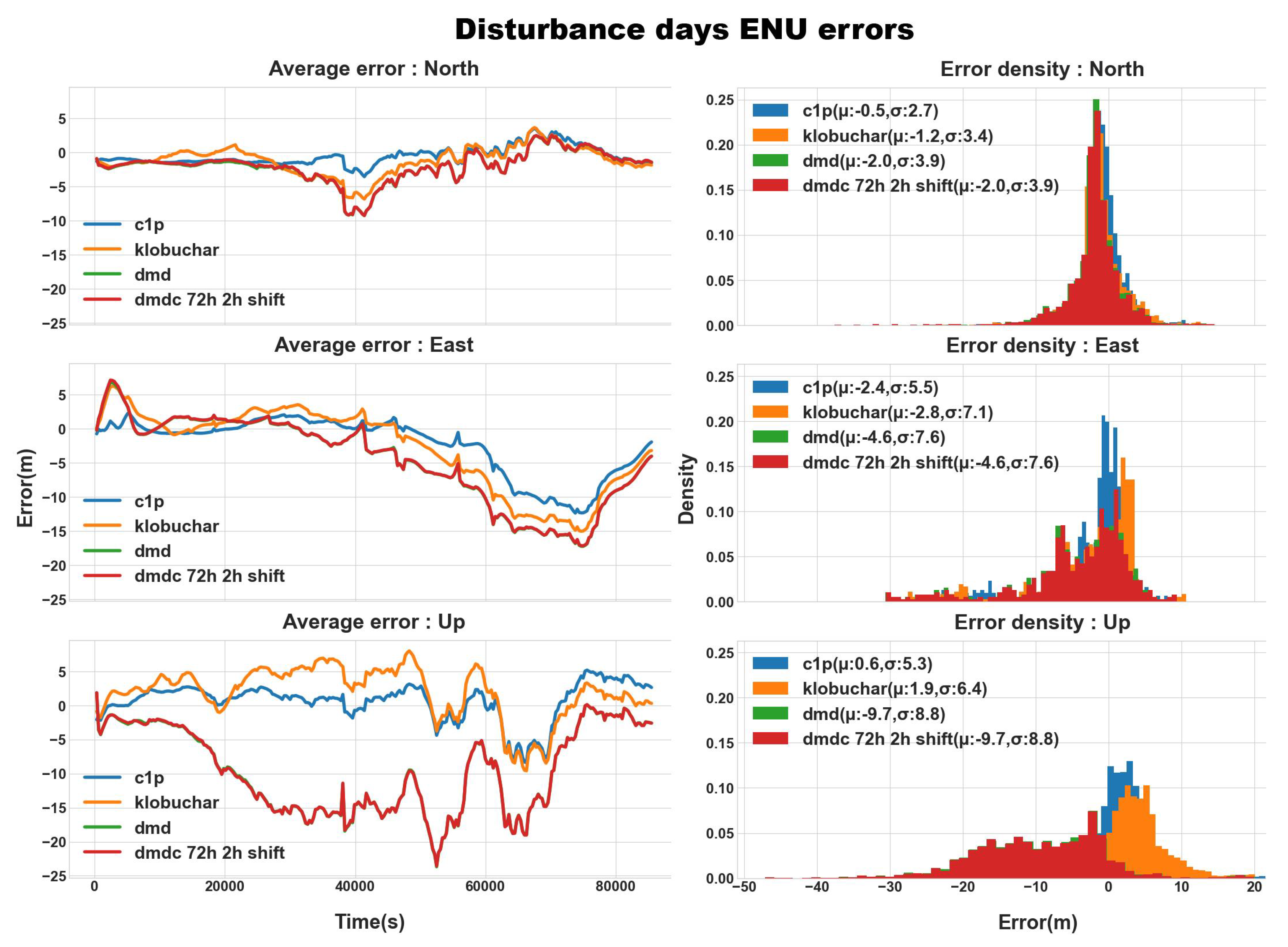
Furthermore, we also examined the quiet and disturbed case studies results using raw Receiver-Independent Exchange Format (RINEX) data afrom a single GNSS station, in order to study the correlation between the vTEC RMSE results and the East-North-Up (ENU) position errors. We estimated the ENU with an open source GNSS-Lab Tool ($gLAB$) software [35]. For every case study, the $gLAB$ software was dfed with a relevant RINEX file, recorded by a receiver located at 32.77899 latitude, 35.02298 longitude and an elevation of 225.1 m. The position solutions were acquired for a L1 single frequency receiver with the following ionospheric correction sources: Klobuchar, C1P, DMD, and DMDc. The best DMDc results, i.e., 2 h $shift$ and 72 h $length$ parameters, were selected as the ionospheric correction. Figure 7 and Figure 8 shows the ENU errors statistics for disturbed and quiet solar periods, respectively, and

Table 3. ENU errors [m] statistics over all time candidates and case studies, sorted by different solar activity periods and error types.

ENU Errors [Meter] Statistics Over All Time Candidates and Study Cases
Period	Stat	Error	DMD	C1P	DMDc(best) with EUV length 72 h and 2 h EUV shift before GIM prediction
Disturbed	AVG	North	−2.03	−0.52	−1.98
		East	−4.63	−2.39	−4.58
		Up	−9.7	0.54	−9.71
	STD	North	3.95	2.71	3.95
		East	7.6	5.49	7.62
		Up	8.82	5.29	−9.71
					DMDc (best) with EUV length 48 h and 8 h EUV shift before GIM prediction
Quiet	AVG	North	−1.4	−0.32	−1.43
		East	−3.14	−1.23	−3.13
		Up	−8.23	1.04	−8.17
	STD	North	2.65	2.18	2.66
		East	4.7	2.81	4.75
		Up	8.12	4.61	8.07

sums up the error statistics for the evaluated ENU case studies.

Finally, we evaluate the Local Ionospheric Maps (LIMs) RMSE of the DMD, DMDc, and C1P compared with the IGS final solution LIMs. Similar to the GIMs vTEC RMSE evaluation, the LIMs RMSE are calculated as the root mean square error between the grid cells of two given maps, for each candidate time step. Figure 9 presents the LIM vTEC RMSE evaluations of DMD, DMDc, and C1P. The main difference between GIM and LIM RMSE is that the LIM RMSE calculation is based only on grid cells along the signal propagation path between the satellite and the receiver, i.e., the intersection grid cells of the signal and the ionosphere (i.e., Ionospheric Pierce Points—IPPs). Figure 10 shows the IPPs at 2-h time intervals for the selected GNSS ground receiver, and

Table 4. Statistics for vTEC LIM RMSE over all time candidates and case studies, sorted by different solar activity periods.

vTEC LIM RMSE [TECU] Statistics Over All Time Candidates and Study Cases
Period	Stat	DMD	C1P	DMDc(best) with EUV length 48 h and 0 h EUV shift before GIM prediction
Disturbed	AVG	4.79	3.67	4.38
	STD	2.47	1.64	1.97
				DMDc(best) with EUV length 48 h and 0 h EUV shift before GIM prediction
Quiet	AVG	4.64	3.87	4.49
	STD	2.75	2.69	2.79
				DMDc(best) with EUV length 48 h and 12 h EUV shift before GIM prediction
CME	AVG	4.08	3.65	3.66
	STD	2.97	3.75	3.66

summarizes the vTEC LIM RMSE statistics. Using this approach, we exclude counting vTEC values which do not contribute to estimating the receiver’s precise location augmented with the relevant ionospheric map corrections.

5. Discussion

Constructing the data set matrix, both for the DMD and DMDc involves fixing the parameter h. As such, we chose its value to be 1440 snapshots (120 days of vTEC GIMs). The selection of such a value is based on the optimization between run time complexity and accuracy. In general, we assume that predictions of 24 h are mostly governed by the dynamics of recent events (up to a scale time of weeks), rather than events which occurred further in past time (such as timescales of months or years). Note that generating ten days of global TEC maps from an X matrix containing 120 days of vTEC maps history takes around 8 min of run-time (based on Intel i9-9900K and 32.0 GB of ram).

The RMSE evaluation of the generated prediction indicated that the DMD and DMDc are capable of estimating future global ionospheric vTEC maps 24 h in advance with 2-h cadence. Moreover, the fact that the DMDc RMSE has an improvement over the DMD suggests that the EUV 126.1 nm time series actually holds relevant information regarding the construction of vTEC in the ionosphere and can be utilized in order to generate more accurate vTEC maps, even with linear models such as the DMDc.

In addition, the analysis of the ENU error distributions, both for quiet and disturbed days, reveals two major insights. The first is that despite the improvement in the RMSE metrics, the DMD and DMDc yield negligible differences with the ENU metrics. The second insight is that across all error statistics, the minima average north position error is 1.1 m, and the minima average east position error is 1.9 m, between the C1P and the DMD. These results do not reflect the statistics achieved by the vTEC GIM RMSE. Table 2, shows that the maxima vTEC GIM RMSE average error between the DMD and C1P (average quiet period) is 0.97 RMSE TECU, meaning that the vTEC mean square error is ∼0.94 TECU, which should correspond to less than 0.16 m error in positioning. Table 3 presents the full ENU position errors statistics. In order to investigate whether the calculated RMSE over the entire vTEC GIM counts for low difference values, and consequently lowers the RMSE scores, we re-evaluated the RMSE score over vTEC LIMs across all case studies. Table 4 presents the full statistics for the LIM RMSE. The vTEC LIM RMSE counts only for vTEC map grid cells, with 5${}^{\circ }$ longitude and 2.5${}^{\circ }$ latitude resolution, which constitutes the IPPs. The vTEC grid cells which correspond to the IPPs are the ones that were utilized as ionospheric corrections with location estimation. Therefore, such evaluation should reveal more accurate correlation between the errors in position estimation and vTEC RMSE. Similarly to the vTEC GIM RMSE, the vTEC LIM RMSE maxima average error was between the DMD and C1P of 1.12 RMSE, which corresponds to ∼1.25 TECU mean square error, and in turn should project ∼0.2 m position error.

6. Conclusions

In this study, we utilized the DMD model in order to evaluate whether it has the ability to predict vTEC GIM for 24 h in advance, with a 2-h candidate time step. In addition, we examined the DMDc approach with external control input, utilizing the EUV time series, under the assumption that future EUV control signals are available. We performed a comprehensive evaluation with twenty-nine different case studies, such that ten cases were chosen during quiet solar activity periods, ten cases were chosen during disturbed solar activity periods, and an additional nine cases were chosen during CME storm events. All evaluations were made using the RMSE metric, whereas the ENU metric was analysed only during quiet and disturbed case studies. All comparisons were made with respect to the IGS final solutions, whereas the C1P 24-h prediction source was considered as a reference model. We successfully applied the DMD model with an ionospheric vTEC maps data set, and constructed a 24-h global ionospheric vTEC map forecast with a 2-h candidate. In addition, we studied the impact of the EUV time series data source with the DMDc framework, indicating improved GIM vTEC RMSE values. Finally, we evaluated the predicted GIMs results with ENU errors metric as an ionospheric correction source for an L1 single-frequency GPS/GNSS solution. Based on these results, we argue that the commonly adopted vTEC map comparison RMSE metric does not entirely reflect the impact with L1 single-frequency positioning solutions using ionospheric corrections, and thus requires further investigation.