Estimations of the Ground-Level NO₂ Concentrations Based on the Sentinel-5P NO₂ Tropospheric Column Number Density Product

Abstract

The main objective of the presented study was to verify the potential of the Sentinel-5 Precursor (S-5P) Tropospheric NO₂ Column Number Density (NO₂ TVCD) to support air pollution monitoring in Poland. The secondary objective of this project was to establish a relationship between air pollution and meteorological conditions. The ERA-5 data together with the NO₂ TVCD product and auxiliary data were further assimilated into an artificial intelligence model in order to estimate surface NO₂ concentrations. The results revealed that the random forest method was the most accurate method for estimating the surface NO₂. The random forest model demonstrated MAE values of 3.4 μg/m³ (MAPE~37%) and 3.2 μg/m³ (MAPE~31%) for the hourly and weekly estimates, respectively. It was observed that the proposed model could be used for at least 120 days per year due to the cloud-free conditions. Further, it was found that the S-5P NO₂ TVCD was the most important variable, which explained more than 50% of the predictions. Other important variables were the nightlights, solar radiation flux, road density, population, and planetary boundary layer height. The predictions obtained with the proposed model were better fitted to the actual surface NO₂ concentrations than the CAMS median ensemble estimations (~15% better accuracy).

1. Introduction

Air pollution is a global threat leading to huge impacts on human health and ecosystems. One of the most dangerous pollutants in the atmosphere is nitrogen dioxide (NO₂). It is responsible for respiratory diseases, cardiovascular diseases, lower self-cleaning airway capacity levels, weakening of the immune function of the lungs, asthma, and many others [1,2]. According to a report by the European Environment Agency (EEA), there were 55,000 premature deaths due to NO₂ across Europe in 2018 [3]. Moreover, high nitrogen concentrations damage ecosystems due to eutrophication and acidification (together with sulfur dioxide, SO₂). This in turn leads to changes in species diversity (reduced levels of existing species and invasions of new ones), as well as to increased concentrations of toxic metals in water and soils [3,4]. In this respect, it is important to monitor the spatiotemporal distribution of NO₂ in order to detect and mitigate high concentrations of this pollutant in the atmosphere. Other air pollutants such as PM_2.5 and PM₁₀ are monitored more than NO₂, especially in Poland. To mitigate this problem, other data sources are needed apart from the in situ measurements. This creates a strong demand for satellite data that allows for timely information gathering on air pollution.

Remote sensing data obtained from space-borne sensors can be used to assess the spatiotemporal distribution of NO₂ at the global scale. The Ozone Monitoring Instrument (OMI) onboard the National Aeronautics and Space Administration (NASA) Aura satellite has been providing daily air pollution data from 2004 at the global scale [5,6]. On the basis of the data provided by the OMI, Jamali et al. [7] found that the globally tropospheric vertical column density (TVCD) of NO₂ featured a slightly increasing trend (0.004⋅10¹⁵ mol/cm²/yr) for the period 2005–2018. The highest increase in NO₂ was observed over India (0.04⋅10¹⁵ mol/cm²/yr) and the highest decrease was observed over Japan (−0.049⋅10¹⁵ mol/cm²/yr). Generally, at the global scale, a statistically significant linear trend was observed over ca. 62% of the Earth, out of which ca. 54% was positive and ca. 8% was negative [7]. In the study performed by Krotkov et al. [8], NO₂ TVCD data from the OMI were analyzed over the most polluted areas around the world. It was found that the NO₂ tropospheric columnar concentrations decreased over the eastern USA by 40% and by 5% over Eastern Europe. On the other hand, increases were observed over China (ca. +5%; however, the trend was expressly negative from 2011), the Middle East (ca. +20%), and India (ca. +50) [8]. Negative trends were observed over eight European cities, including Athens, Bucharest, Lisbon, Paris, Rome, Rotterdam, Berlin, and Madrid, for the period 2005–2014 [9]. Georgoulias et al. [10] studied NO₂ TVCD trends derived from the records of four satellite sensors, namely the Global Ozone Monitoring Experiment (GOME) sensor onboard the second European Remote Sensing satellite (ERS-2), the Global Ozone Monitoring Experiment 2 (GOME-2) sensor onboard Meteorogical Operation A (Metop-A), the GOME-2 sensor onboard Meteorogical Operation B (MetOp-B), and the Scanning Imaging Absorption Spectrometer for Atmospheric Cartography (SCIAMACHY) sensor onboard the Environmental Satellite (Envisat). The key findings from this study related to negative trends observed during the twenty-one years (1996–2017) over the most industrialized and highly populated regions of the well-developed countries and positive trends over developing regions [10]. In contrast to Jamali et al. [7], Georgoulias et al. [10] claimed that linear trends are not reliable on a global scale for a such long period [10].

The major advancement in satellite observations of NO₂ was the TROPOspheric Monitoring Instrument (TROPOMI) instrument mounted onboard the Sentinel-5 Precursor satellite (Sentinel-5P, S-5P) launched by the European Space Agency [11]. NO₂ atmospheric pollution has been even more threatening since the COVID-19 pandemic started, and many scientific studies have elaborated on this topic. In this respect, reduced NO₂ levels in 2020 were reported by Bauwens et al. [12] at the global and regional scales. They analyzed NO₂ TVCD data over 33 cities all over the world, and only over 1 city (Isfahan) did the atmospheric NO₂ concentration increase during the pandemic [12]. It was claimed that the reason for this increase was related to ignoring COVID-19 restrictions in Iran [12].

The satellite NO₂ column number density or tropospheric column number density is a different physical quantity than the ground concentration expressed in parts per million (ppm) or µg/m³. The physical relation between both quantities is usually complicated due to the vertical variability of NO₂ concentrations. A vertical profile of NO₂ depends on many factors, including the weather conditions, emissions, and chemical reactions. However, it is known that the satellite NO₂ TVCD is related to the surface concentrations, as the main NO₂ sources are related to human ground activities and the lifetime of NO₂ is short, which in turn precludes transportation at long distances [13,14,15]. Since the launch of the OMI in 2004, many studies on the modeling of NO₂ concentrations at the surface have been conducted by assimilating various NO₂ TVCD satellite products. Sentinel-5P data have also been used to estimate this kind of pollution. The research performed by Griffin et al. [16] over the Canadian Oil Sands revealed a linear relationship between the TROPOMI NO₂ TVCD and ground mass concentration of NO₂ characterized by a Pearson correlation coefficient (R) of 0.67 [16]. A higher R coefficient (0.85) was observed by Zheng et al. [17], who studied monthly means of NO₂ derived from Sentinel-5P and in situ measurements for different districts in China. Analogously, Cerosimo et al. [18] used the monthly mean S-5P NO₂ TVCD product to retrieve the surface NO₂ concentrations over Italy. However, in this study, the authors did not average the measurements over the districts and used measurements from single stations instead, as opposed to Zheng et al. [17]. Cerosimo et al. [18] reported values of R² = 0.85 (TROPOMI NO₂ vs. ground concentration) over the north of Italy and R² = 0.71 over the south of Italy. In addition, Cerosimo et al. [18] also performed an analysis on non-averaged data that revealed values of R² = 0.50 over the south of Italy and R² = 0.42 over the north of Italy. A similar coefficient of determination (R² = 0.48 for hourly data and R² = 0.77 for annual data) was found by Jeong and Hong [19] for surface NO₂ concentrations retrieved from the S-5P TVCD NO₂ product over South Korea. Due to an undeniable relationship between atmospheric concentrations of pollutants and meteorological conditions [20,21,22,23,24], as well as anthropogenic factors [23,25,26,27,28], they are often assimilated into the ML-based NO₂ retrieval models together with satellite NO₂ products. In this respect, the study carried out by Kim et al. [29] over the north of Italy, Switzerland, Austria, and southeast France, based on the XGboost method [30], revealed different agreements between the modeled NO₂ concentrations and in situ measurements, depending on the averaging interval, i.e., R²~0.45 for hourly data, R²~0.55 for daily averaged data, and R²~0.60 for weekly and monthly averaged data [29]. Kim et al. [29] found that the S-5P TVCD NO₂ product had a relative impact of 12% on the estimation of surface NO₂ concentrations. Only traffic emissions had a higher impact (14,8%). Other predictors that influenced the surface NO₂ values by more than 10% were the time of day (11.5%) and planetary boundary layer height (PBLH: 11.4%) [29]. Wang et al. [31] employed five machine learning methods for the estimation of surface NO₂ atmospheric concentrations over China based on NO₂ TVCD data together with ancillary data (land cover, normalized difference vegetation index (NDVI), road density, and population density). Wang et al. [31] reported values of R² = 0.72 for light gradient boosting (Light-GBM) [32], R² = 0.68 for the XGBoost method [30], R² = 0.57 for the random forest (RF) method [33], R² = 0.55 for the deep belief network (DBN) method [34], and R² = 0.43 for the BPNN (back propagation neural network) method [35]. The surface NO₂ was predicted by Chan et al. [36] using the S-5P TVCD, planetary boundary layer height, digital elevation model (DEM), air temperature, wind speed, relative humidity, precipitation, and incoming shortwave radiation flux at the surface level as predictors. They used an artificial neural network (ANN) algorithm [37] that featured a correlation value of R² = 0.64 [36]. Analogously, Kim et al. [29] studied the impact of each predictor on the accuracy of the surface NO₂ estimation. Chan et al. [36] also found that the S-5P NO₂ TVCD was the most significant variable when estimating surface NO₂ concentrations [36]. From the perspective of inconsistent results in surface NO₂ modeling and the different impacts of the explanatory variables (e.g., meteorological, anthropogenic) reported by the aforementioned studies, it is necessary to conduct consecutive studies to better define the limitations in the modeling of atmospheric NO₂ concentrations based on satellite data, meteorological conditions, and anthropogenic factors. This challenge was the main motivation to conduct this study and to address the following research questions:

• How much does the accuracy of surface NO₂ modeling improve if the S-5P TCVD NO₂ product is assimilated into a model?
• What are the impacts of the meteorological conditions and anthropogenic factors on the NO₂ modeling results?
• What are the impacts of the temporal averaging of NO₂ retrievals and in situ measurements on the overall accuracy?
• Which machine learning models provide the most accurate NO₂ estimations?
• What was the accuracy of the latest S-5P TROPOMI TCVD NO₂ product version 2.3.1 released on 16 December 2021 [38]?

The main objective of this study was to verify the potential of a machine learning (ML) approach based on the NO₂ TVCD Sentinel-5P satellite product generated by the European Space Agency (ESA) to support air pollution monitoring in Poland. In this respect, the surface atmospheric NO₂ concentration modeled by means of the ML algorithm was validated against in situ measurements provided by the Chief Inspectorate of Environmental Protection (GIOS). The secondary objective of the study was to establish a relationship between NO₂ air pollution (based on Sentinel-5P products) and the ERA5 meteorological reanalysis provided by the European Center for Medium-Range Weather Forecasts (ECMWF).

The analyses were performed for two temporal aggregation levels, namely hourly and weekly data, to determine the impact of the temporal averaging. Furthermore, several ML algorithms were tested together with a simple linear regression model to select the most robust method. Ultimately, the impacts of the explanatory variables on the model results were analyzed to determine the most significant variables.

This manuscript is structured into five sections. The Section 1 provides a comprehensive literature overview on the modeling of surface atmospheric NO₂ concentrations. Section 2 provides descriptions of the data used within the study, as well as the methodology for the data processing, analysis, and validation. Section 3 provides the results of the conducted analysis. Section 4 provides a discussion of the acquired results, while Section 5 concludes the conducted study.

2. Materials and Methods

2.1. Study Area

Poland was used as the study area to develop a NO₂ retrieval algorithm and to analyze the spatial distribution of NO₂. The climate in Poland is temperate. It is oceanic in the northwest and more continental towards the southeast. The average temperature in summer is ca. 20 °C, while in winter it is ca. −1 °C [39]. The topography of Poland has a latitudinal belt-like layout, with a young glacial landscape (with a belt for part of the country and lake districts) in the northern part of the country, an old glacial landscape in some parts, and a belt of highlands and mountains on the ground. The lowlands cover 91.3% of the area, the highlands 5.6%, and the mountains 3.3%, of which 0.2% are high mountains [40]. The above factors all make Poland a perfect representative of a temperate climate zone. Moreover, other Central and Eastern European countries are facing similar problems and challenges related to air quality as Poland. There is a similar annual mean mass concentration of NO₂ in Poland of 15.6 µg/m³ to the other countries of the region, e.g., Czechia with 15.5 µg/m³, Croatia with 13.8 µg/m³, Slovakia with 14.8 µg/m³, Hungary with 17.0; µg/m³, Serbia with 17.3 µg/m³, and Slovenia with 14.5 µg/m³ [3].

2.2. Materials

The modeling of the surface NO₂ mass concentration presented in this study was based on in situ NO₂ measurements, the Sentinel-5P TVCD NO₂ product, the ERA-5 meteorological reanalysis from the Copernicus Climate Change Service (CCS), and various ancillary datasets, such as for the nightlight intensity derived from the Visible Infrared Imaging Radiometer Suite (VIIRS) satellite instrument, population density, road density, and DEM. The study covered the period from 1 July 2018 to 30 July 2021.

2.2.1. NO₂ Tropospheric Vertical Column Density (NO₂ TVCD) Product Retrieved from Sentinel-5P Satellite TROPOMI Measurements

The Sentinel-5P satellite was launched on 13 October 2017 as part of the Copernicus Earth Observation Program. The S-5P mission supports the global monitoring of the atmosphere and air quality using TROPOMI. The TROPOMI instrument consists of four spectrometers measuring radiation in the ultraviolet (270–320 nm), visible (310–500 nm), near-infrared (675–775 nm), and shortwave infrared (2305–2385 nm) electromagnetic spectrums. At the beginning of the mission, the spatial resolution of the TROPOMI products was 3.5 km × 7 km, while currently (December 2022) it is 3.5 km × 5.5 km. The width of the swath is 2600 km, which allows for daily monitoring of the atmosphere at the global scale. The spectral resolutions of the TROPOMI products vary from 1 nm in the UV band through to 0.5 nm in the VIR and NIR bands and 0.25 nm in the SWIR band [11].

The NO₂ TVCD product is generated by the Royal Netherlands Meteorological Institute (KNMI) by means of DOMINO [41,42] and Quality Assurance for Essential Climate Variables (QA4ECV) [43] algorithms. These methods share three common steps:

• The NO₂ slant column densities are retrieved from the measured radiance and irradiance spectra using the differential optical absorption spectroscopy (DOAS) method;
• The separation of tropospheric and stratospheric columns, i.e., their conversion to tropospheric and stratospheric slant columns;
• The conversion of tropospheric and stratospheric slant columns into tropospheric and stratospheric vertical column densities [42,44].

The vertical profiles of NO₂ are calculated for the center of a pixel featuring a spatial resolution of 1° × 1° and are based on the chemistry transport model (CTM)—TM5-MP [44,45]. Finally, the filtering of the cloud cover is performed using the Fast Retrieval Scheme for Clouds from the Oxygen A-Band (FRESCO-S) algorithm [46].

Within this study, the reprocessed Sentinel-5P TROPOMI NO₂ product (S5P-PAL) was used (version 2.3.1), which covers the period from 1 July 2018 to 30 June 2021 [38]. The NO₂ TVCD values are expressed in mol/m². The NO₂ TVCD, acquisition time, and quality flag (qa_value) data were obtained using Climate Data Operator (CDO) software [47] and scripts written in the R programming language based on the raster package [48], ncdf4 package [49], and rgdal package [50].

This allowed us to filter the NO₂ TCVD values, with the data qa_values > 0.75, as suggested by van Geffen et al. [44] and Ialongo et al. [14] being used. Consequently, the majority of the cloudy pixels (cloud radiance fractions > 0.5) and pixels covered by snow or ice were removed [51].

2.2.2. In Situ Air Quality Measurements

The NO₂ surface mass concentration was obtained from the Chief Inspectorate of Environmental Protection (GIOS). The GIOS provides hourly averages of measurements recorded every 10 s at a height of 2 m a.g.l. The number of stations where NO₂ is measured is constantly changing, as some new ones are added and some old ones are discontinued. In this respect, 136 locations were selected featuring NO₂ measurement records collected since 2018. Further, stations classified as transport (roadside) and industrial stations were excluded from the analysis because traffic-related and industrial-related pollutants can vary substantially within a few meters, and such stations are not representative of a large satellite footprint [36,52,53]. Thus, the data from 116 stations, including 20 non-built-up stations, 12 suburban stations, and 84 urban stations, were used within this study [40]. The spatial distribution of the stations in Poland measuring atmospheric NO₂ concentrations is dominated by urban areas, as there are only few background stations in Poland (Figure 1).

Due to the high daily variability of NO₂ [54,55], the hourly means provided by GIOS were linearly interpolated to the time of the S-5P image acquisition.

2.2.3. Meteorological Data

The meteorological conditions have a great impact on the air quality [20,21,22,23,24,29,30]; thus, they were also used as explanatory variables to predict the NO₂ concentrations in this study. In this respect, the following meteorological variables were analyzed: the air temperature (T), dew point temperature (DT), atmospheric pressure (P), surface incoming solar radiation accumulated over one hour (RAD), U zonal wind component (U WIND), V meridional wind component (V WIND), and PBLH. The T and DT were used to calculate the relative humidity (RH), while the U WIND and V WIND were used to calculate the wind speed (WS) and wind direction (WD). These datasets were retrieved from the ERA5-Land Hourly reanalysis model provided by the European Center for Medium-Range Weather Forecasts (ECMWF) at the 0.1° × 0.1° spatial resolution [56]. The meteorological data, excluding PBLH, were retrieved using the Google Earth Engine (GEE) [57], while the PBLH data were obtained using an R programming language script using the ecmwfr package [58]. The ERA5-Land data were linearly interpolated to the time of the S-5P acquisition in order to reduce temporal inconsistencies between meteorological and satellite data. Then, linearly interpolated datasets were spatially downscaled to the 3.5 km × 5.5 km spatial resolution using bilinear interpolation [59,60,61].

The meteorological datasets were used to derive the zonal atmospheric circulation index values over Poland according to the classification method proposed by Lityński [62,63,64]. In this respect, the values for sea-level pressure from the NCEP/NCAR (National Centers for Environmental Prediction/National Center for Atmospheric Research) reanalysis were used. The circulation types (CT) were distinguished using 3 main indices (zonal, Ws; meridional, Wp; cyclonicity index, Cp), which in turn were subdivided into 27 circulation types. The Ws and Wp were calculated based on differences in atmospheric pressure between zones at 40°–65°N and 0°–35°E, while the Cp was the atmospheric pressure over the node nearest to Warsaw (52.5°N, 20°E) subtracted by 1000 hPa [62,63,64]. Over the years, the synoptic maps used by Lityński were replaced by NCEP/NCAR reanalysis data [65,66,67].

2.2.4. Ancillary Data

NO₂ emissions are greatly related to anthropogenic activities [13,14,15,68,69]. In this respect, it was necessary to add anthropogenic explanatory variables to train the NO₂ retrieval model, such as population density, road density, and satellite data on the intensity of nightlights. In order to obtain information about the population density, the Global Human Settlement Layers (GHSL) dataset was used for the year 2015. This dataset contains the population density expressed as the number of people within a 250 m × 250 m spatial grid [70]. Additionally, the intensity of nightlights was used, as it corresponds well with socioeconomic dynamics [71,72,73]. This dataset consists of nighttime radiance imagery acquired by the Visible Infrared Imaging Radiometer Suite (VIIRS) Day/Night Band (DNB) [74,75]. These two datasets were extracted from the GEE [57] at a spatial resolution of 464 m × 464 m. The road density was derived from the OpenStreetMap dataset [76]. The population density and road density were calculated as the sum of people within a 3.5 × 5.5 grid and the road density was calculated as the total length of the roads within a grid.

Following recommendations from studies on NO₂ modeling [29,30], the digital elevation model (DEM) from the Shuttle Radar Topography Mission (SRTM) featuring a 30 m × 30 m spatial resolution [77] was used in this study. The information on the terrain elevation was extracted from the GEE [57].

Ultimately, the surface atmospheric NO₂ concentrations from the CAMS (Copernicus Atmosphere Monitoring Service) reanalysis were used to benchmark the NO₂ retrieval models proposed within this study. The CAMS dataset covers the period from 10 November 2018 to 30 June 2021 and consists of an ensemble median of 11 CAMS models considered as the best-fitted to real concentrations among other models [78,79]. The temporal resolution of the CAMS ensemble median is 1 h, while the spatial resolution is 1 km × 1 km. Estimates are provided at 10 vertical levels (surface, 50 m, 100 m, 250 m, 500 m, 750 m, 1000 m, 2000 m, 3000 m, 5000 m). The data are provided for Europe only [80]. In contrast to other data, the CAMS ensemble median NO₂ estimates were not resampled to the resolution of Sentinel-5P pixels so as not to distort the comparable results.

2.3. Methods

2.3.1. Modeling of Surface NO₂ Mass Concentration

In order to predict the surface NO₂, we used the datasets mentioned in Section 2.2. In this respect, the NO₂ TVCD, T, P, RAD, WS, PBLH, NIGHTLIGHT, POPULATION, ROADS DENSITY, and ELEVATION were included in the models. Moreover, the atmospheric circulation data (CT), as a categorical factor, were included in the machine learning methods.

Four kinds of methods were used:

• Linear regression with one independent variable (LM)—NO₂ TVCD;
• Multiple linear regression with several independent variables (MLM)—NO₂ TVCD, T, P, RAD, WS, PBLH, NIGHTLIGHT, POPULATION, ROADS DENSITY, and ELEVATION;
• Random forests with several independent variables (RF)—NO₂ TVCD, T, P, RAD, WS, PBLH, NIGHTLIGHT, POPULATION, ROADS DENSITY, ELEVATION, and CT;
• Radial kernel support vector machine with several independent variables (SVM)—NO₂ TVCD, T, P, RAD, WS, PBLH, NIGHTLIGHT, POPULATION, ROADS DENSITY, ELEVATION, and CT.

Prediction analyses were performed for two periods: hourly data (for hours of each available S5-P image) and weekly data (weekly averaged data). Each variable was averaged to the weekly mean.

One parameter was chosen to point out outliers within the dataset and exclude them:

• Stations measuring surface NO₂ closer than 100 m from the road (2 stations; 1024 observations; 2% of all observations).

According to Section 2.2.2, transport stations were excluded from the analysis [36,52,53]. However, there were still stations located close to the roads within the dataset. Due to the excessive noise concentrations over the stations next to the roads (and defined as background stations), these were also excluded from the dataset [81].

After excluding the outliers, the datasets consisted of 50,099 hourly observations and 13,765 weekly observations, having been reduced by 1024 observations (2%) and 994 observations (7%), respectively.

In order to perform prediction activities, the dataset was divided into two parts: a training dataset used for the training model and a test dataset used for validation. The training dataset consisted of data for January, March, May, July, September, and November, while the testing dataset consisted of data for February, April, June, August, October, and December. Due to our approach, the models were trained and validated over datasets that differed from each other. The training dataset and testing dataset included 22,678 (45%) and 27,421 (55%) hourly observations, respectively, and 7126 (52%) and 6639 (48%) weekly averages, respectively.

To obtain information about the availability of useful S-5P observations, we counted the number of observations characterized by qa_values > 0.75 for each pixel within the study area. Only data for 2019 and 2020 were chosen for the observation analysis as they were the only fully covered years in the study’s analysis period.

2.3.2. Validation methodology

The results obtained from the formulated predictions models were validated using the following statistical parameters:

• R-squared (R²):

$${\mathrm{R}}^2=1-\frac{{\displaystyle \sum }{\left({\mathrm{y}}_{\mathrm{i}}-{\hat{\mathrm{y}}}_{\mathrm{i}}\right)}^2}{{\displaystyle \sum }{\left({\mathrm{y}}_1-\overline{\mathrm{y}}\right)}^2}$$

(1)

• Mean squared error (MSE):

$$\mathrm{MSE}=\frac{1}{\mathrm{n}}{{\displaystyle \sum }}_{\mathrm{i}=1}^{\mathrm{n}}{\left({\mathrm{y}}_{\mathrm{i}}-{\hat{\mathrm{y}}}_{\mathrm{i}}\right)}^2$$

(2)

• Root mean squared error (RMSE):

$$\mathrm{RMSE}=\sqrt{\frac{1}{\mathrm{n}}{{\displaystyle \sum }}_{\mathrm{i}=1}^{\mathrm{n}}\frac{{\left({\mathrm{y}}_{\mathrm{i}}-{\hat{\mathrm{y}}}_{\mathrm{i}}\right)}^2}{\mathrm{n}}}$$

(3)

• Bias:

$$\mathrm{BIAS}=\frac{1}{\mathrm{n}}{{\displaystyle \sum }}_{\mathrm{i}=1}^{\mathrm{n}}\left({\mathrm{y}}_{\mathrm{i}}-{\hat{\mathrm{y}}}_{\mathrm{i}}\right)$$

(4)

• Mean absolute error (MAE):

$$\mathrm{MAE}=\frac{1}{\mathrm{n}}{{\displaystyle \sum }}_{\mathrm{i}=1}^{\mathrm{n}}\left|{\mathrm{y}}_{\mathrm{i}}-{\hat{\mathrm{y}}}_{\mathrm{i}}\right|$$

(5)

• Mean percentage absolute error (MAPE):

$$\mathrm{MAPE}=\frac{1}{\mathrm{n}}{{\displaystyle \sum }}_{\mathrm{i}=1}^{\mathrm{n}}\frac{\left|{\mathrm{y}}_{\mathrm{i}}-{\hat{\mathrm{y}}}_{\mathrm{i}}\right|}{{\mathrm{y}}_{\mathrm{i}}}$$

(6)

Here, y_i is the actual value, ŷ_i is the predicted value, $\overline{\mathrm{y}}$ is the mean for the actual values, and n is the number of observations.

Considering that the data used for prediction purposes were expressed in various units, we performed the normalization before the modeling. We used standardization feature scaling in order to bring all values into the common scale:

$$\mathrm{z}=\frac{\mathrm{x}-ⲙ}{\mathsf{\sigma }}$$

(7)

Here, z is the standardized variable, x is the non-standardized variable, ⲙ is the mean of the non-standardized variable, and σ is the standard deviation of the non-standardized variable.

2.3.3. Ranking the Modeling Skills of the Selected Predictors

The variables’ importance for multilinear regression was calculated by comparing the standardized regression coefficients. The standardized coefficients were also summed. Further, the percentage of each variable within the total was calculated [82].

The variables’ importance for the random forest model was calculated with the randomForest package created for the R programming language, and the variables’ contribution was expressed by the mean increase in MSE, divided by a measure of the variability (%IncMSE), which was calculated as follows:

• Compute the model’s MSE;
• For each variable in the model:

(a)

Permute the variable;

(b)

Calculate the new model MSE according to the variable permutation;

(c)

Take the difference between the model MSE and new model MSE;

3.

Collect the results in a list;

4.

Rank the variables’ importance according to the %IncMSE values, whereby the greater the value, the more important the variable [83].

This method is considered more reliable than the decrease in node impurity [84,85].

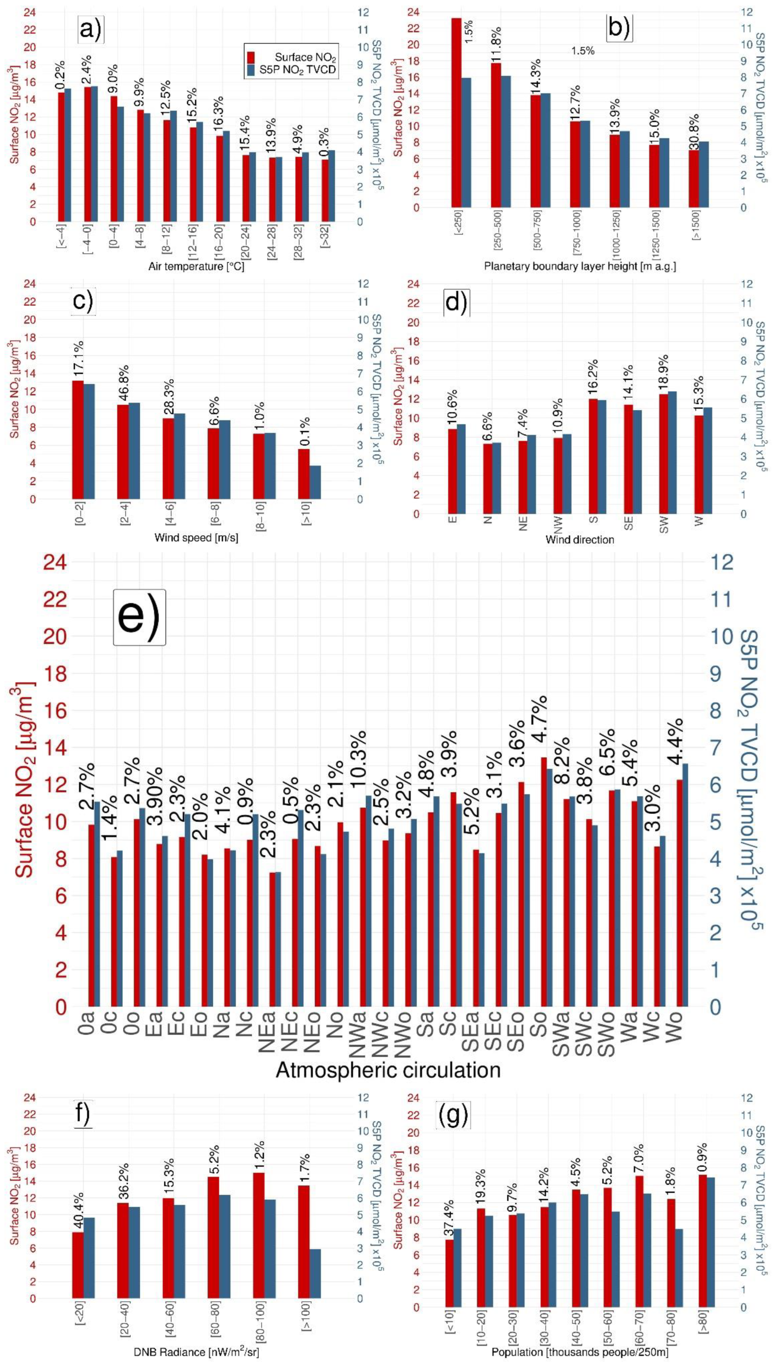
2.3.4. Determining the Variability of the NO₂ TVCD and Surface NO₂ with Respect to the Meteorological Conditions and Anthropogenic Factors

There were verified changes in the surface concentrations of NO₂ and NO₂ TVCD due to different meteorological conditions (T, PBLH, P, WS, WD, CTYPE), as well as anthropogenic and geographical factors (nightlights and population). The means of the NO₂ pollution levels (surface and columnar) were calculated for the following intervals:

• 2 °C for T;
• 250 m above ground for PBLH;
• 2 m/s for WS;
• N, S, E, W, SE, SW, NW, and NE for WD;
• 27 types of atmospheric circulations;
• 20 nW/cm²/sr for NIGHTLIGHT;
• People/km for POPULATION.

3. Results

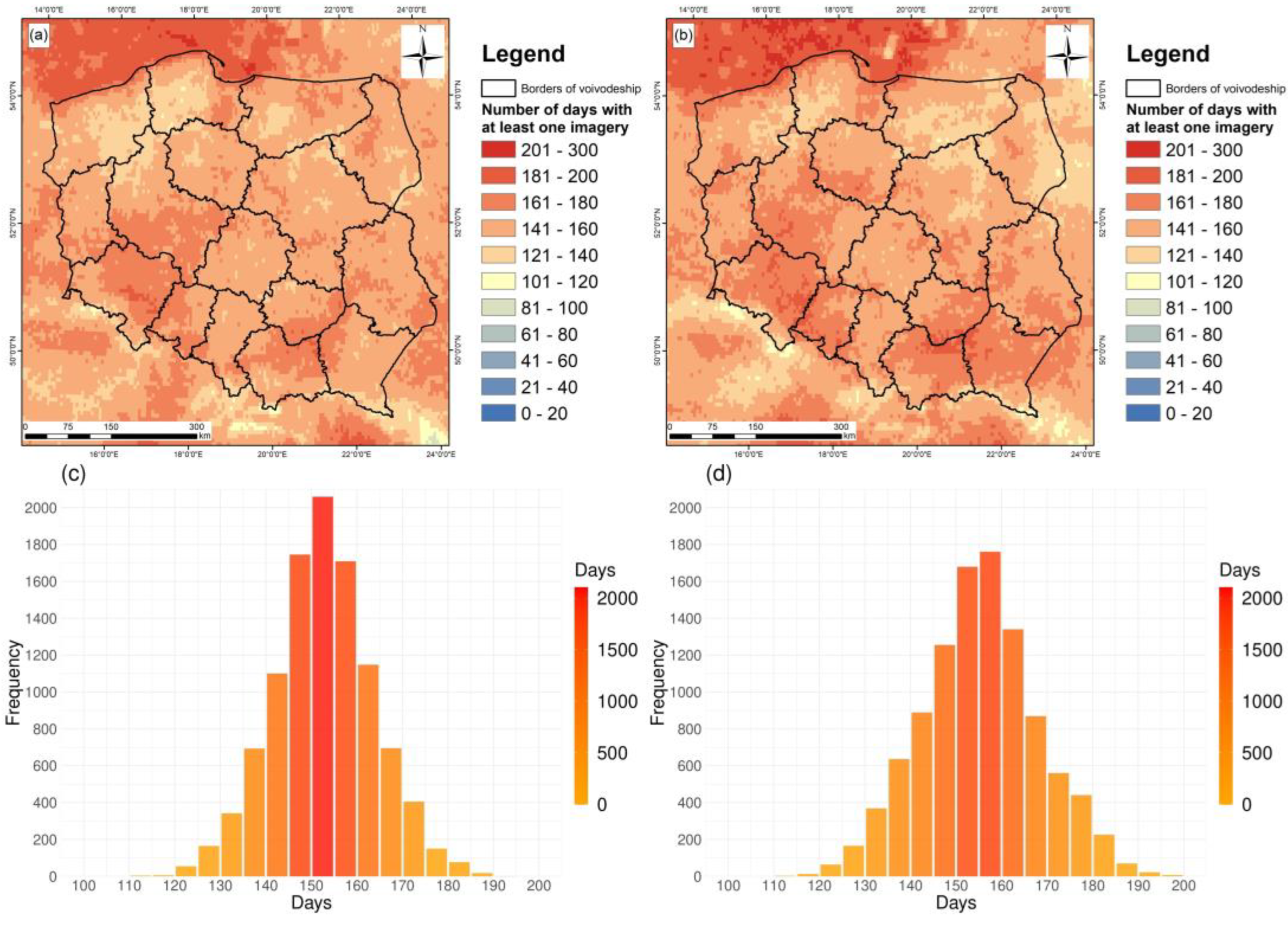
3.1. Numbers of Observations

First of all, the limitations of using satellite S-5P data due to cloud coverage were verified. As mentioned in Section 2.2.1, only available observations for 2019 and 2020 were calculated.

The numbers of cloud-free observations over Poland depended on the location. The highest numbers of such observations were observed both in 2019 and 2020 over the southwestern part of Poland (170–180 observations in 2019, 190–200 observations in 2020) and over the southeastern part of Poland (150–160 observations in 2019 and 190–200 observations in 2020). The lowest numbers of cloud-free observations were noticed over the northern part of Poland near the Baltic Sea area, where only 130–140 observations were noted in 2019 and 2020. Additionally, the area near the northeastern border was characterized by low numbers of cloud-free images; there were 130–140 cloud-free observations in each year (Figure 2a,b). Thus, the frequency rates of cloud-free pixels within the borders of Poland were similar in 2019 and 2020. For each part of Poland, it was possible to obtain data for at least one-third of the year. For the areas in the southern part of Poland, it was even possible to obtain data for more than half of the year.

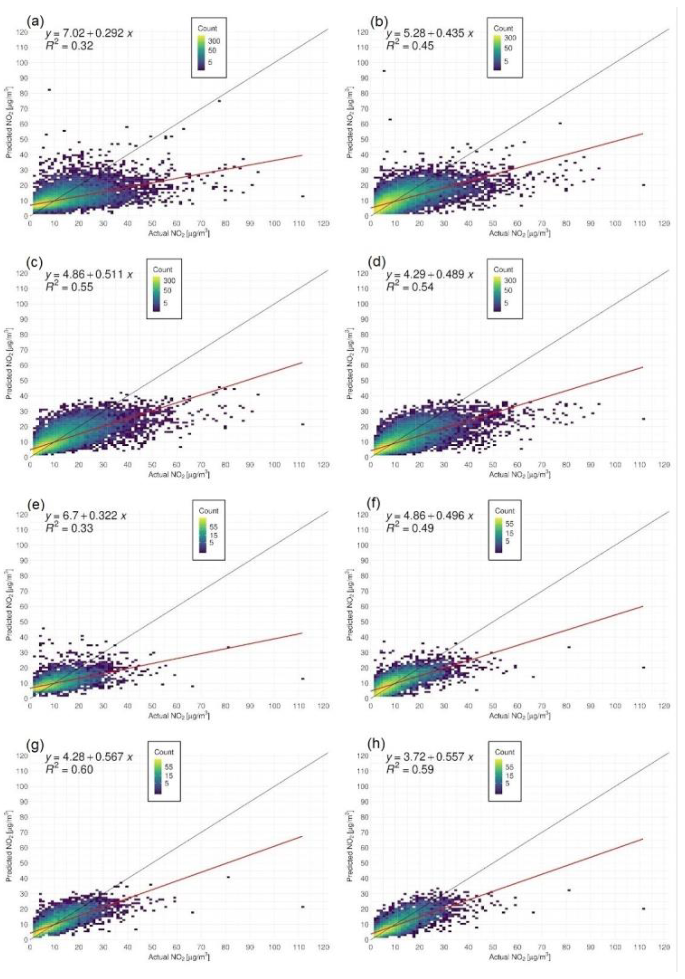
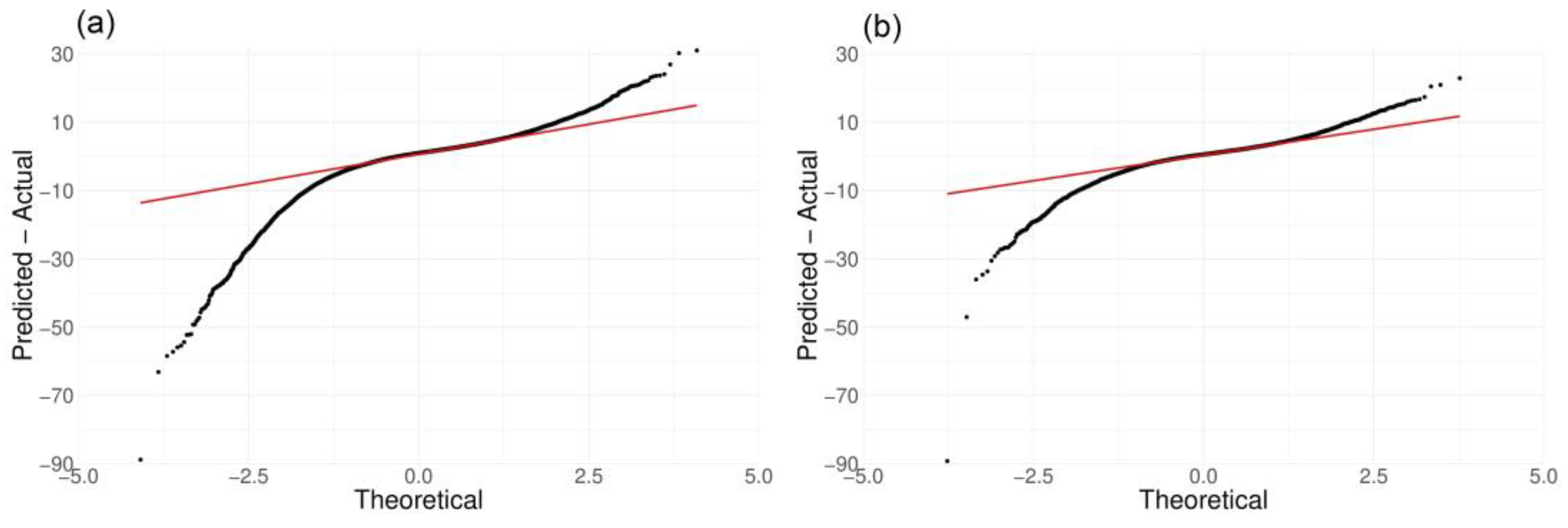
3.2. Modeling of Surface NO₂ Mass Concentration

The modeling of the surface NO₂ was the main objective of the study. The results and validation of estimated surface NO₂ mass concentrations based on satellite, meteorological, and other data are listed in Section 2.2.

Firstly, a linear model with one independent variable—NO₂ TVCD—was used to estimate the surface NO₂ mass concentrations (LM-S5P). The results demonstrated that R² = 0.32 with MAE and MAPE values of 4.9 μg/m³ and 48.4% for the hourly estimates, respectively. LM-S5P was the only model with an RMSE higher than 7.00 μg/m³ for these measurements. The accuracy of the model was absolutely unsatisfactory. The results were slightly better for the weekly averages. LM-S5P gave results of R² = 0.33, RMSE = 6.2 μg/m³, MAE = 4.3 μg/m³, and MAPE = 42.4% (

Table 1. Statistics of prediction of NO₂ surface mass concentration with use of various techniques: LM-S5P—Linear regression with one independent variable (NO₂ derived by Sentinel-5P); MLM—Multiple linear regression with several independent variables; RF—Random forest; SVM—Support Vector Machine.

	Surface NO2 Mass Concentration Estimations [µg/m3]
			MEAN	MIN	MAX	SD	1st Q	3rd Q
Testing dataset (n = 27,241)			10.1	<0.1	111.4	8.9	4.4	13.1
Training dataset (n = 22,678)			10.4	<0.1	100.6	8.6	4.4	12.9
		METHOD	R2	MSE	RMSE [µg/m3]	Bias [µg/m3]	MAE [µg/m3]	MAPE [%]
Hourly measurements		LM-S5P	0.32	53.2	7.3	0.1	4.9	48.4
		MLM	0.45	43.1	6.6	0.4	4.2	42.1
		RF	0.53	34.8	5.9	<0.1	3.7	37.2
		SVM	0.54	37.7	6.1	1.0	3.7	36.9
		METHOD	R2	MSE	RMSE [µg/m3]	Bias [µg/m3]	MAE [µg/m3]	MAPE [%]
Weekly averages		LM-S5P	0.33	38.1	6.2	0.1	4.3	42.4
		MLM	0.49	29.0	5.4	0.2	3.6	35.5
		RF	0.60	23.1	4.8	−0.1	3.1	30.8
		SVM	0.59	24.3	4.9	0.8	3.2	31.2

). However, it was decided to develop a model with more independent variables.

The second approach involved multilinear regression with ten variables (MLM). The estimates were more accurate in comparison with LM-S5P. We observed values of R² = 0.45, RMSE = 6.6 μg/m³, MAE = 4.2 μg/m³, and MAPE = 42.1% for the hourly data and R² = 0.49, RMSE = 5.4 μg/m³, MAE = 3.6 μg/m³, and MAPE = 35.5% for the weekly averages (Table 1). This method allowed us to verify the influence of each variable in the model. A detailed description of the impact of the variables is given in Section 3.3.

To improve the model and make it possible to include categorical data, a machine learning approach was used. Firstly, estimates were calculated with the use of the random forest (RF) method. This approach achieved R² values higher than 0.50 for the hourly data and 0.60 for the weekly averages. The MAE declined to 3.7 μg/m³ for the hourly measurements and to 3.1 μg/m³ for the weekly averages, which corresponded to 37.2% and 30.8%, respectively (Table 1). This model was more accurate, especially for the group of high predicted values but low actual values. For the LM-S5P model and MLM, the observed estimates were in the range of ca. 40–80 μg/m³, while the actual values were lower than 10 μg/m³ (Figure 3a,b). The RF method handled these measurements and predicted them with higher accuracy (Figure 3c). Additionally, the group of estimations between the black line and red line (Figure 3,b), which corresponded to actual values > 50 μg/m³ (Figure 3a,b), was predicted with higher accuracy using the RF approach for the hourly data as well as for weekly averages (Figure 3c,g). Therefore, it seems that the RF method was less sensitive for non-typical actual surface NO₂ mass concentrations, which compounded the results of the LM-S5P and MLM method.

The second machine learning approach used for modeling purposes was the radial kernel support vector machine (SVM). The results and accuracy were very similar in comparison with the RF model at R² = 0.54, RMSE = 6.1 μg/m³, MAE = 3.7 μg/m³, and MAPE = 36.9% for the hourly estimates and R² = 0.59, RMSE = 4.9μg/m³, MAE = 3.2 μg/m³, and MAPE = 31.2% for the weekly averages (Table 1). Significant differences in estimates between the RF and SVM methods were observed within the interval ranges of 70–90 μg/m³ for the actual (ground-based observation) values and 30–50 μg/m³ for the predicted values (Figure 3c,d,g,h). The predictions calculated using the SVM method were slightly higher.

Figure 3 shows that all of the models overestimated the surface NO₂ mass concentrations during relatively clean conditions (NO₂ values less than approximately 10 μg/m³) and underestimated the values during pollution events.

To sum up, the development of the linear model into a more complex model requiring more computing power was justified. The multilinear model revealed significantly better estimation accuracy than the linear model with one independent variable (ca. 6%), while the machine learning approaches were ca. 5% more accurate than the multilinear model (for the hourly observations). For the weekly averages, the tendencies were similar. The MLM model was ca. 7% more accurate than the LM-S5P model, while the RF and SVM estimates had accuracy values higher than ca. 5% in comparison with the MLM model. Therefore, the SVM method was a little bit more accurate for hourly estimates, while the RF method was more accurate for weekly averages (Table 1). However, one approach was chosen for further investigation—the RF model (for hourly and weekly data). This was decided due to the very low differences between the SVM and RF models, which actually may have been random and due to the lower bias for the RF model (<0.1. μg/m³ and −0.1 μg/m³ for hourly and weekly predictions, respectively) (Table 1). Moreover, computing estimates using the RF method is faster and requires a computer with less computing power, which makes the method more applicable for further studies.

The distribution and magnitude of differences between the predicted NO₂ mass concentrations (RF model) and actual surface NO₂ concentrations are shown in Figure 4. A perfect fit would be described by points placed strictly on the red line. Figure 4 allows for easy visualization and interpretation of how many values are underestimated (points below the red line) and overestimated (over the red line). In this study, the differences were characterized by an asymmetric distribution. The magnitude of the underestimations was higher than the magnitude of the overestimations (Figure 4). For the hourly estimates, this trend is even more evident, as the tails are bigger and deviate more from the perfect fit (red line). Differences higher than 50 μg/m³ can even be observed (Figure 4a), while for the weekly averages a poor number of differences higher than 30 μg/m³ can be noticed (Figure 4b). Additionally, the increase in overestimations is less smooth and the peaks are higher, at ca. 30 μg/m³ for hourly and ca. 15 μg/m³ for weekly estimates (Figure 4).

Considering that the function for the estimations was fitted above the perfect fit for actual values lower than ca. 10 μg/m³ and under the perfect fit for actual values higher than ca. 10 μg/m³ (Figure 3c,g), it was decided to verify the bias within the quartiles defined by the actual surface NO₂ mass concentrations. It was found that the proposed random forest model overestimated the results, with 2.5 μg/m³ and 2.2 μg/m³ bias rates for hourly and weekly predictions within the first quartile (

Table 2. Bias [μg/m³] for estimations performed by RF model within the quartiles both for hourly measurements and weekly averages.

	1st Q	2–3rd Q	4th Q
Hourly measurements	2.5	1.7	−5.1
Weekly averages	2.2	1.3	−4.0

), which was 4.4 μg/m³ (Table 1). Even if the bias rates show a high relative difference, it has to be emphasized that a NO₂ mass concentration of ca. 4–5 μg/m³ is still a very low level of air pollution. Whether or not the model was biased at ca. 2–2.5 μg/m³, the results still showed a very low level of NO₂. The estimates within the second and third quartiles were less biased at 1.7 μg/m³ and 1.3 μg/m³ for the hourly and weekly NO₂ mass concentrations, respectively (Table 2). This is extremely important because it was the most frequent observed level of NO₂ pollution. It also corresponds well to Figure 3c,g, where the perfect fit and modeled fit are the closest around the values defined by the second and third quartiles (Table 2). The highest bias rates were observed within the fourth quartile, which were −5.1 μg/m³ and −4.0 μg/m³ for the hourly and weekly predictions, respectively (Table 2). Therefore, these underestimations for the high actual values of the NO₂ mass concentrations were considered the most serious problem within the proposed model. Such results are expected, while satellite columnar observations tend to average the pollution data in comparison to one-level (surface) concentration. Therefore, all models underestimated the range of surface concentrations of NO₂. Since this was also a problem that had occurred within the other studies, this issue was analyzed and is discussed in Section 4.

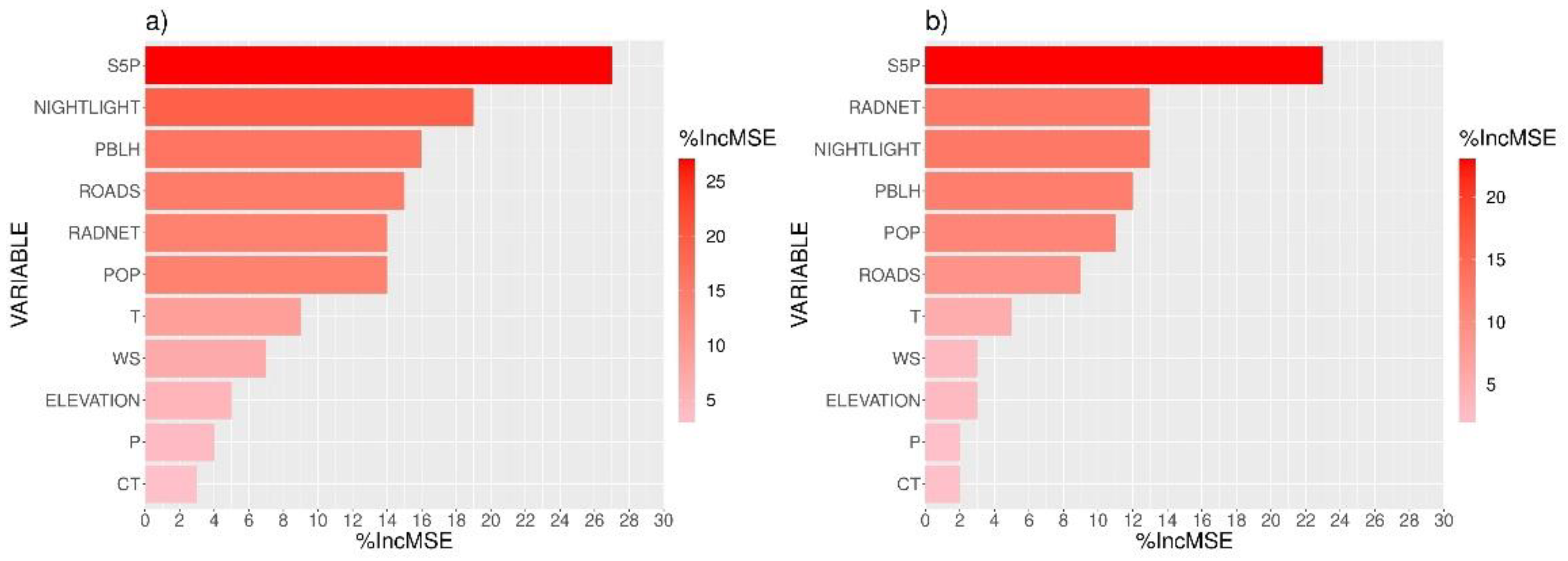
3.3. Variables’ Importance

With respect to

Table 3. Variables’ coefficients used for multilinear regression.

Variable	S5P	T	P	RAD	WS	PBLH	NIGHTLIGHT	POP	ROADS	ELEVATION	INTERCEPT
Coefficient hourly	0.62 (57%)	−0.01 (1%)	−0.03 (3%)	−0.06% (6%)	−0.07 (6%)	−0.08 (7%)	0.05 (5%)	0.03 (3%)	0.06 (6%)	0.01 (1%)	0.07 (6%)
Coefficient weekly	0.69 (53%)	−0.04 (3%)	−0.04 (3%)	−0.06 (5%)	−0.07 (5%)	−0.10 (8%)	0.06 (5%)	0.04 (3%)	0.08 (6%)	0.01 (1%)	0.10 (8%)

, for the hourly estimates, the most important variable for the prediction of surface NO₂ mass concentrations was NO₂ TVCD obtained from S-5P. It explained 57% of the model’s results. The second most significant variable was PBLH, which explained 7% of the results. RAD, WS, ROADS, and NIGHTLIGHT were the other variables that explained at least 5% of the results, at 6%, 6%, 6%, and 5%, respectively. The rest of the meteorological factors, T and P, explained less than 5% of the results. However, they were still statistically significant (p-value < 0.05). POP explained 3%. Therefore, 57% of the model’s results were explained by the TROPOMI data, 23% were explained by the meteorological data (T, P, WS, RAD, PBLH), and 14% by the anthropogenic factors (NIGHTLIGHT, POP, ROADS); 1% was explained by the elevation and 6% by an intercept.

The increases in the TVCD of NO₂, nightlights, population, road density, and elevation gave rise to increased surface NO₂ mass concentrations, while the increases in temperature, pressure, radiation, wind speed, and PBLH caused decreased surface NO₂ mass concentrations. To sum up, it seems that the meteorological factors were favorable to decreases in surface NO₂ values. In contrast, anthropogenic factors increase the surface NO₂ mass concentration (Table 3).

Very similar results were obtained for the weekly averages. Here, 53% of the model’s results were explained by the S-5P data. Again, the second most important variable was BLH (8%). Generally, the meteorological data expressed 24% of the model’s results, while 14% was expressed by anthropogenic factors. Additionally, 1% of the predictions were determined by the elevation and 8% by the intercept (Table 3).

An investigation of the variables’ importance within the RF model was conducted and the results are expressed as % changes in the MSE. Because the RF model allows for using categorical data, it was possible to verify the impacts of factors such as the circulation type (CT).

For the hourly measurements, just like with the multilinear approach, the most important variable for the RF model was the S-5P TVCD of NO₂. The decrease in accuracy when excluding S-5P from the model was 27%. The next most significant variable was NIGHTLIGHT (19% decrease in accuracy). The other variables that decreased accuracy by at least 15% when excluded from the model were PBLH (16%) and ROADS (15%). Beside PBLH, the meteorological factor that affected the accuracy the most was RAD (14% decrease in accuracy). POP was almost as important (an almost 14% decrease in MSE). When excluding other factors from the RF model, the accuracy decreased by less than 10% (T, 9%; WS, 7%; ELEVATION, 5%; P, 4%). The lowest impact on the model accuracy was for CT; removing CT from the model increased the MSE by 3% (Figure 5a). Thus, it seems that no additional factor such as CT influenced the quality of the RF model in comparison with the MLM model except for the method itself. In contrast with their importance within the MLM model, the anthropogenic factors (NIGHTLIGHT, ROADS, POP) were more important for the RF approach (Table 3).

Slightly different results were revealed for the weekly averages. TVCD of NO₂ and NIGHTLIGHT were again the most important factors (23% and 13% decreases in accuracy, respectively, when excluded from the model). On the other hand, RAD and POPULATION were more important than ROADS (13% and 11% decreases in accuracy, respectively). Still, PBLH had a significant impact on the model (12% increase in MSE when excluded). Again, T, WS, ELEVATION, and P were the least important with 5%, 3%, 3%, and 2% decreases in accuracy, respectively (Figure 5b). It is worth mentioning that the impacts of WS and P were lower for the weekly averages estimations than the hourly estimations, while with the MLM approach, the opposite was true (Table 3). Regardless, according to their importance and influence on the MSE, two groups of variables are emphasized for the RF model (both for the hourly and weekly data):

• Those with an impact higher than or equal to 10% on the changes in MSE: S5P, NIGHTLIGHT, PBLH, ROADS, RAD, and POP;
• Those with an impact lower than 10% on the changes in MSE: T, P, WS, ELEVATION, and CT.

3.4. Changes in NO₂ TVCD and Surface NO₂ Mass Concentration in Respect to Meteorological Conditions and Other Factors

The changes in NO₂ TVCD and surface NO₂ mass concentration values were verified as indicators of pollution in each interval defined for each meteorological or anthropogenic factor.

A decrease in air temperature implied a decrease in air pollution (TVCD of NO₂ as well as surface NO₂). Starting at −4–0 °C, the surface NO₂ fell consistently to 24–28 °C and then it increased until the last interval (Figure 6a). The slight increase starting from 24–28 °C was supposedly induced by photochemical reactions that started to occur with the high solar radiation flux and high air temperature [86]. In contrast, the surface NO₂ mass concentration stopped rising at the 8–12 °C range and then fell further at 24–28 °C. Just like the surface NO₂, it increased again in the next two intervals. On average, the surface NO₂ concentration dropped by 0.8 μg/m³ in each subsequent interval, while the NO₂ TVCD concentration dropped by 0.7 × 10⁵ μmol/m² in each subsequent interval. The biggest changes were noticed for the 20–24 °C range, which were −2.2 μg/m³ for the surface NO₂ and −2.4 × 10⁵ μmol/m² for the TVCD of NO₂. The first interval (below −4 °C) seemed to be out of sync because there was a poor number of observations (lower than 1% of all observations). For the same reason, it was hard to unequivocally interpret results for the >32 °C interval (Figure 6a).

The meteorological parameter with the greatest effect on air pollution was PBLH (Section 3.3). A trend of decreasing air pollution with increasing PBLH values was observed. This can be explained by deeper convective mixing of the air pollution emitted at the surface. One exception was the first interval (0–250 m a.g.) for the TVCD of NO₂; however, only 1.5% of all observations were covered within this interval. The average decrease in the surface NO₂ mass concentration was 2.7 μg/m³ with PBL at elevations higher than 250 m, while the average decrease in the TVCD of NO₂ was 1.3 × 10⁵ μmol/m² with PBL at elevations higher than 250 m (Figure 6b).

A significant decrease in air pollution was also observed with increasing wind speed. The surface NO₂ mass concentration decreased by 1.5 μg/m³ on average with a WS increase of 2 m/s, while the columnar density decreased by 1.8 × 10⁵ μmol/m². The greatest drops were observed between the first and second intervals at 2.7 μg/m³ and 2.1 × 10⁵ umol/m², respectively. There was a greater decrease between 8–10 m/s and >10 m/s for the satellite NO₂ values; however, only 0.1% of all observations were collected under such conditions (Figure 6c).

There were also observed differences in surface NO₂ and NO₂ TVCD values for different advections. This was confirmation that the air is cleaner during northern advections. This is caused by the movement of relatively clean Atlantic air masses from the north and the inflow of more polluted air masses from the south. Additionally, the eastern wind direction was more favorable for lower TVCD and surface NO₂ values than the western advections (Figure 6d). As was mentioned previously, NO₂ is mostly generated by human activities, and beyond the western border of Poland there are many human settlements. On the other hand, beyond the eastern border there are more forests, arable lands, grasslands, and wetlands.

The dependence above was confirmed by the distribution of surface NO₂ concentration and NO₂ TVCD with respect to the circulation types. Therefore, the pollution was higher during southern and western circulations, while the lowest pollution was observed during the northern and eastern circulations. Additionally, the pollution was higher during gradientless circulations (suffix o) when the air masses were slack and air mixing was obstructed (Figure 6e).

As was already pointed out, the anthropogenic factors were also very significant for the distribution of NO₂ pollution. We found positive trends of 0.9 μg/m³ and 0.7 × 10⁵ μmol/m² increases in surface concentration and columnar NO₂ density, respectively, with increases in population density for the 10,000 people per pixel. However, these trends were not so evident or constant. We observed an exception for the 70–80,000 people-per-pixel interval, which was characterized by evident decreases in surface and columnar NO₂. On the other hand, it was hard to interpret these two last intervals due to the poor numbers of observations, representing 1.8% and 0.9% of all observations, respectively. Moreover, it was assumed that in such areas, there was a lot of residential construction and a lower road density, positively influencing the NO₂ emissions [23,29,31]. Regardless, a significant trend of increasing NO₂ was observed for growing populations (Figure 6g).

The nighttime radiance was the last analyzed variable with respect to changes in NO₂ concentration and columnar density. The tendency of the two types of air pollution was positive for the surface NO₂ but was negative for the TVCD. For the surface NO₂, we observed a 1.1 μg/m³ increase per 20 nW/m²/sr, while we observed an average 0.8 × 10⁵ μmol/m² decrease per 20 nW/m²/sr for TROPOMI NO₂. However, poor numbers of observations could lead to misleading conclusions. The last two intervals covered only 1.2% and 1.7% of the total, respectively. If they were excluded from the analysis, the trends for both the surface and satellite-measured NO₂ would be positive (Figure 6f).

To sum up, changes in NO₂ pollution, for both the surface mass concentration and columnar density, were observed with respect to the different meteorological conditions and anthropogenic factors. PBLH was the variable that was distinguished by the highest change in air pollution through the intervals. It corresponded well with the RF model and MLM model, which were strongly dependent on the PBLH. Additionally, lower air temperatures implied higher air pollution. This corresponded well with the significant impact on the model by the RAD, which was strictly connected to the temperature but also connected to the PBLH. Furthermore, it was confirmed that the wind speed affected the NO₂ pollution. A higher wind speed implied a lower surface NO₂ concentration and TVCD of NO₂. The analysis on the advections and circulation types confirmed that southern and western advections implied higher levels of NO₂. Finally, we affirmed the influence of human activities and settlements, with higher population densities and higher radiance levels due to nightlights being linked to increases in NO₂.

4. Discussion

Chan et al. [36] performed similar research for Germany, which is quite climatically similar to Poland. They found a value of R² = 0.64 using a neural network approach. However, they compared the daily averaged surface mass concentration of NO₂ to the daily averaged NO₂ TVCD, so their result is not fully comparable with our results [36]. Chan et al. [36] also verified the impact of each variable on their model. Both our results and their results show that the TVCD of NO₂ is the most important variable when trying to synergize satellite, meteorological, and geographical data in order to estimate surface pollution concentrations. On the other hand, the second most important variable in the mentioned study was elevation, which was one of the least important variables in our model. It is supposed that Germany has a more varied topography, so that variable has more influence. What is interesting is that in Chan et al.’s study, the impact of the PBLH on the model was very low [36]. For the proposed RF model, the PBLH was the most important meteorological variable for hourly estimates and the second one for weekly estimates. This finding corresponds with the results reported by Kim et al. [29], who found that the PBLH was the most important meteorological factor (4th most important of all variables) in their model. In contrast, they claimed that the solar radiation influenced the results least in their model, while for the proposed model it was as important as the PBLH. However, for modeling purposes they used the hour and day of the year, for which the solar radiation was a kind of derivative [29]. Thus, the influence of the solar radiation could be explained by those two variables. The validation of the model performed by Kim et al. [29] showed a value of R² = 0.59, which was similar to our results. Again, just like in our study and Chan et al.’s study [36], the model proposed by Kim et al. [29] tends to underestimate the surface NO₂ for highly polluted days. However, they claimed that this was intentional in order to optimize the predictions for mean concentrations [29]. In other studies, in which only the NO₂ TVCD was used to the estimate surface NO₂, worse results were achieved, including R² = 0.45 in Griffin et al.’s study [16] and R² = 0.48 in Jeong and Hong’s study [19]. In the only study on TROPOMI NO₂ performed for Poland, Kawka et al. [87] compared NO₂ TVCD with surface NO₂ concentrations estimated using the GEM-AQ model [88] with the use of averaging kernels derived from the S-5P datasets [87]. They estimated monthly averages, so their results cannot be compared with our results. However, it was pointed out that the estimates were more accurate when PBLH data were added to the model [87].

Our estimates were also compared to estimates provided by the CAMS model for the ensemble median of the models. Because of the availability of the CAMS data (over a three-year rolling archive), a comparison was performed for the 10 November 2018–30 June 2021 period. In this respect, the MAE, MAPE, and R² values of the RF model could be different from the values in Section 3.2.

The comparison revealed that the proposed RF model estimated surface NO₂ concentrations with ca. 15% better accuracy than the CAMS ensemble median model (ca. 1.5 μg/m³). The R² for the RF model was 0.08 higher than the R² for the CAMS model. Both the RF model and CAMS model generally underestimated the NO₂ surface mass concentrations (

Table 4. Comparison of RF and CAMS ensemble median models’ statistics.

	R2	MAE [μg/m3]	MAPE [%]
RF MODEL	0.54	3.9	40.0
CAMS	0.46	5.4	52.7

).

Figure 7 shows the spatial distribution and variability of the modeled surface NO₂ concentrations obtained from the RF model (Figure 7a,c), which were developed within the study, as well as the predictions derived from the CAMS model (ensemble median) (Figure 7b,d). The overall distribution of the surface NO₂ mass concentrations is quite similar across the years and methods. The most polluted areas, around cities such as Warszawa, Lodz, Katowice, Krakow, and Wroclaw, are distinguished by surface NO₂ ca. concentrations of ca. 10 μg/m³ by both the RF and CAMS models. However, there are differences over the other capital cities (smaller cities) such as Bialystok, Olsztyn, Lublin, Rzeszow, and Gorzow Wielkopolski. In 2019 and 2020, the RF model (Figure 7a,c) indicated a slightly higher NO₂ level than the CAMS ensemble median (Figure 7b,d). In Figure 7a,c, single pixels can be observed over these cities (which clearly differ from the surrounding areas), which cannot be observed in Figure 7b,d. Moreover, the same situation can be observed for Bydgoszcz and Torun in 2020. According to the RF model, a mass concentration range of 4–6 μg/m³ NO₂ was observed for these cities, while in the neighborhoods it was 2–4 μg/m³. The CAMS ensemble median indicated that in Torun and Bydgoszcz, as well as around these cities, the surface NO₂ concentrations were 4–6 μg/m³. At this point, it should be remembered that NO₂ is strictly connected to human activities, so the air pollution in the city should be higher than in the surrounding area. Thus, it is claimed that the proposed RF model is more sensitive in estimating surface NO₂ mass concentrations over human settlements. On the other hand, the CAMS ensemble median (Figure 7b,d) estimated higher surface NO₂ concentrations than the RF model (Figure 7a,c) over the area that starts from Warsaw and passes through Lodz, then reaches Katowice and Krakow. This is where one of the busiest motorways in Poland is located. It seems that the CAMS ensemble median is more sensitive to linear traffic emissions.

The model developed within this study is distinguished by its better accuracy (Table 4) and spatial recognition for surface NO₂ concentrations than the CAMS (ensemble median) model (Figure 7). However, it must be remembered that the CAMS model provides data on many pollutants. Moreover, the CAMS data are provided hourly. The RF model created within the study is dependent on satellites, so it is impossible to predict surface NO₂ concentrations every day using the described approach.

The proposed RF model is prone to similar aberrations as the models used in previous studies; high surface NO₂ mass concentrations are underestimated while very low values (<5 μg/m³) are overestimated [29,31,36,87,89]. The previous studies did not indicate specific reasons for this but pointed out that it was characteristic of the modeling of NO₂ mass concentrations in itself. Underestimations of high values and overestimations of low values were also observed for the ensemble median model estimates provided by CAMS [90,91]. It is assumed that the main reason for the underestimations in the proposed random forest model’s results is the underestimation of columnar values of NO₂ provided by the Sentinel-5P measurements, which was the most important variable within the model. The underestimation of the columnar density is a widely known issue that has been described many times since the launch of S-5P. It was described in studies on Sentinel-5P NO₂ concentrations [38,92]. Moreover, it was observed by Griffin et al. [16] in a study performed over Canada, by Ialogno et al. [14] in a study performed over Finland, and by Liu et al. [93] in a study performed over China. Thus, this issue has been observed all over the world. Regarding the reasons for underestimations, these include the coarse resolution of the a priori-derived profiles (1° × 1°), aerosol impacts, uncertainties regarding the cloud fraction [86], and the size of the TROPOMI resolution for the atmospheric mass factor (AMF), which cannot resolve street-level variations in concentrations [94]. As such, algorithms dedicated to providing columnar NO₂ concentrations from TROPOMI have been developed. This was the motivation for reprocessing the Sentinel-5P TROPOMI NO₂ product (S5P-PAL) with the algorithm from version 2.3.1, which was supposed to improve the accuracy of the NO₂ column density estimates over the most polluted areas [38]. Underestimations of the TVCD of NO₂ had been also found for data derived by the OMI [94,95,96] and GOME [97]. As a reason for the overestimation of low values, it has been indicated that during clear-sky conditions, which are also relatively clean air conditions, the AMF is underestimated and the NO₂ TVCD is overestimated [98].

To sum up, the proposed model underestimates high values and overestimates surface NO₂ mass concentrations. The estimates for the second and third quartiles were quite similar to the actual values. This corresponded well with the other studies and models. The fact that the problem has appeared within studies using the TROPOMI as well as the OMI and GOME means that the issue is caused by the satellite measurement itself, and not by the method of prediction. In contrast to the previous studies, the factors with the greatest effects on the estimates were different for the Polish study area. This led to the conclusion that in different regions, different variables are the most significant for the surface NO₂ mass concentrations.

5. Conclusions

This study aimed to estimate NO₂ surface mass concentrations based on columnar NO₂ obtained from Sentinel-5P measurements, meteorological conditions, and anthropogenic and geographical factors. Four approaches, including linear regression, multilinear regression, and machine learning methods such as random forest (RF) and support vector machine, were used to achieve the goal of this research. The estimations were performed with respect to the time ranges (hourly and weekly).

It was found that the random forest (RF) and support vector machine (SVM) models were the most accurate methods for estimating surface NO₂ concentrations. However, the RF model was chosen as the best solution as it was faster and required a computer with less computing power, making it applicable for further usage. The RF model demonstrated MAE values of 3.4 μg/m³ (MAPE~37%) and 3.2 μg/m³ (MAPE~31%) for the hourly and weekly estimates, respectively (Section 3.2). It also has to be pointed out that the ground measurements may have been influenced by some errors. In particular, the location of a certain station may not be representative for the whole pixel area, in addition to the significant NO₂ equipment uncertainty. In fact, the proposed model may be more accurate than is described by the statistics. Furthermore, it was observed that the RF model could be used for at least 120 days per year due to the cloud-free conditions. However, areas with ca. 180 days a year with favorable conditions for estimation were distinguished (southern–western Poland) (Section 3.1).

The variables’ impact on the estimations was also verified. It was found that the S-5P TVCD of NO₂ was the most important variable, which explained more than 50% of the predictions. Other important variables were the nightlights, solar radiation flux, road density, population, and planetary boundary layer height (PBLH). The impact of the PBLH was particularly significant, as suggested by Kawka et al. [87]. They used only TROPOMI data, but they suggested using the PBLH in further research. The data quantity of the proposed model was quite similar to previous studies performed for other areas [16,19,29,36] (see Section 4). Importantly, the predictions obtained with the proposed RF model were better fitted to the actual surface NO₂ concentrations than the CAMS median ensemble estimations (ca. 15% better accuracy), which suggested that the RF model is more accurate for the area of Poland.

Changes in NO₂ pollution, both in terms of the surface mass concentration and columnar density, were observed with respect to various meteorological conditions. The most significant changes were observed for the increase in PBLH when the air pollution decreased by 2.7 μg/m³ at 250 m (Figure 5b). Additionally, lower air temperatures and lower wind speeds implied higher air pollution. Moreover, western and southern advections as well as atmospheric circulations were favorable to higher levels of NO₂ (Section 3.4).

To conclude, the key findings of this research were as follows:

• There were at least 120 days per year when it was possible to perform model calculations for Poland using TROPOMI observations;
• The results revealed that the machine learning methods (RF and SVM) gave ca. 63% accuracy for hourly estimations of NO₂ and 69% accuracy for weekly averages;
• The implementation of meteorological and anthropogenic variables improved the quality of the models. The MLM approach gave 6% (hourly) and 7% (weekly) lower MAPE values than the LM-S5P approach, while the RF and SVM approaches gave 11% (hourly) and 12% (weekly) lower MAPE values than the LM-S5P approach;
• The planetary boundary layer height, solar radiation, nightlights, roads density, and population influenced the estimations the most;
• The air temperature, wind speed, surface pressure, elevation, and type of atmospheric circulation influenced the estimations the least;
• The trends for the surface NO₂ and TVCD of NO₂ were negative for increases in air temperature, PBLH, and wind speed, while they were positive for increases in population and nightlights;
• The RF model created within the study was better fitted to the actual values than the CAMS ensemble median model.

The conclusions drawn from this study will be further used to improve the model and to verify its accuracy for other areas. Our attention was paid to the issue of the station’s representativeness. Thus, in further research, we will verify the station’s representativeness with respect to the area of the TROPOMI pixel. In addition, information on the vertical variability of the NO₂ concentrations (especially at the PBL and above) could improve the estimations of the surface concentrations. For this purpose, drone observations will be used to determine the NO₂ profiles and to improve our models.

References

1. Sroczyński, J. The Impact of Atmos. In Air Pollution on Human Health; PAN: Wrocław, Poland, 1988. (In Polish) [Google Scholar]
2. World Health Origination. WHO Air Quality Guidelines for Particulate Matter, Ozone, Nitrogen Dioxide and Sulfur Dioxide. Available online: https://apps.who.int/iris/handle/10665/345329 (accessed on 10 October 2021).
3. European Environment Agency. Air Quality in Europe—2020. Report. EEA Report No 9/2020. Available online: https://www.eea.europa.eu/publications/air-quality-in-europe-2020-report (accessed on 10 October 2021).
4. Duprè, C.; Stevens, C.J.; Ranke, T.; Bleeker, A.; Peppler-Lisbach, C.O.R.D.; Gowing, D.J.; Dise, N.D.; Dorland, E.; Bobbkink, R.; Diekmann, M. Changes in species richness and composition in European acidic grasslands over the past 70 years: The contribution of cumulative atmospheric nitrogen deposition. Glob. Chang. Biol. 2010, 16, 344–357. [Google Scholar] [CrossRef]
5. Schoeberl, M.R.; Douglass, A.R.; Hilsenrath, E.; Bhartia, P.K.; Beer, R.; Waters, J.W.; Gunson, M.R.; Fridevaiux, L.; Gille, J.C.; Barnett, J.J.; et al. Overview of the EOS Aura mission. IEEE Trans. Geosci. Remote Sens. 2006, 44, 1066–1074. [Google Scholar] [CrossRef] [Green Version]
6. National Aeronautics and Space Administration-OMI Science Team. OMI/Aura Level 2 Nitrogen Dioxide (NO2) Trace Gas Column Data 1-Orbit subset Swath along CloudSat track 1-Orbit Swath 13x24 km, Edited by GES DISC, NASA Goddard Space Flight Center, Goddard Earth Sciences Data and Information Services Center (GES DISC). 2012. Available online: https://disc.gsfc.nasa.gov/datasets/OMNO2_CPR_003/summary (accessed on 20 October 2022).
7. Jamali, S.; Klingmyr, D.; Tagesson, T. Global-scale patterns and trends in tropospheric NO2 concentrations, 2005–2018. Remote Sens. 2020, 12, 3526. [Google Scholar] [CrossRef]
8. Krotkov, N.A.; McLinden, C.A.; Li, C.; Lamsal, L.N.; Celarier, E.A.; Marchenko, S.V.; Swartz, W.H.; Bucsela, W.J.; Joiner, J.; Duncan, W.N.; et al. Aura OMI observations of regional SO 2 and NO 2 pollution changes from 2005 to 2015. Atmos. Chem. Phys. 2016, 16, 4605–4629. [Google Scholar] [CrossRef] [Green Version]
9. Paraschiv, S.; Constantin, D.E.; Paraschiv, S.L.; Voiculescu, M. OMI and ground-based in-situ tropospheric nitrogen dioxide observations over several important European cities during 2005–2014. Int. J. Environ. Res. Public Health 2017, 14, 1415. [Google Scholar] [CrossRef] [Green Version]
10. Georgoulias, A.K.; van der A, R.J.; Stammes, P.; Boersma, K.F.; Eskes, H.J. Trends and trend reversal detection in 2 decades of tropospheric NO2 satellite observations. Atmos. Chem. Phys. 2019, 19, 6269–6294. [Google Scholar] [CrossRef] [Green Version]
11. Veefkind, J.; Aben, I.; McMullan, K.; Förster, H.; de Vries, J.; Otter, G.; Claas, J.; Eskes, H.; de Haan, J.; Kleipool, Q. TROPOMI on the ESA Sentinel-5 Precursor: A GMES mission for global observations of the Atmos. composition for climate, air quality and ozone layer applications. Remote Sens. Environ. 2012, 120, 70–83. [Google Scholar] [CrossRef]
12. Bauwens, M.; Compernolle, S.; Stavrakou, T.; Müller, J.; Van Gent, J.; Eskes, H.; Levelt, P.F.; van der A, R.; Veefkind, J.P.; Vlietinck, J.; et al. Impact of Coronavirus Outbreak on NO2 Pollution Assessed Using TROPOMI and OMI Observations. Geophys. Res. Lett. 2020, 47, e2020GL087978. [Google Scholar] [CrossRef]
13. Qin, K.; Rao, L.; Xu, J.; Bai, Y.; Zou, J.; Hao, N.; Li, S.; Yu, C. Estimating ground level NO2 concentrations over Central-Eastern China using a satellite-based geographically and temporally weighted regression model. Remote Sens. 2017, 9, 950. [Google Scholar] [CrossRef] [Green Version]
14. Ialongo, I.; Virta, H.; Eskes, H.; Hovila, J.; Douros, J. Comparison of TROPOMI/Sentinel-5 Precursor NO2 observations with ground-based measurements in Helsinki. Atmos. Meas. Tech. 2020, 13, 205–218. [Google Scholar] [CrossRef]
15. Kang, Y.; Choi, H.; Im, J.; Park, S.; Shin, M.; Song, C.K.; Kim, S. Estimation of surface-level NO2 and O3 concentrations using TROPOMI data and machine learning over East Asia. Environ. Pollut. 2021, 288, 117711. [Google Scholar] [CrossRef] [PubMed]
16. Griffin, D.; Zhao, X.; McLinden, C.A.; Boersma, F.; Bourassa, A.; Dammers, E.; Degenstein, D.; Eskes, H.; Fehr, L.; Fioletov, V.; et al. High resolution mapping of nitrogen dioxide with TROPOMI: First results and validation over the Canadian oil sands. Geophys. Res. Lett. 2019, 46, 1049–1060. [Google Scholar] [CrossRef] [PubMed] [Green Version]
17. Zheng, Z.; Yang, Z.; Wu, Z.; Marinello, F. Spatial variation of NO2 and its impact factors in China: An application of sentinel-5P products. Remote Sens. 2021, 11, 1939. [Google Scholar] [CrossRef] [Green Version]
18. Cersosimo, A.; Serio, C.; Masiello, G. TROPOMI NO2 tropospheric column data: Regridding to 1 km grid-resolution and assessment of their consistency with in situ surface observations. Remote Sens. 2020, 12, 2212. [Google Scholar] [CrossRef]
19. Jeong, U.; Hong, H. Assessment of tropospheric concentrations of NO2 from the TROPOMI/Sentinel-5 Precursor for the estimation of long-term exposure to surface NO2 over South Korea. Remote Sens. 2021, 13, 1877. [Google Scholar] [CrossRef]
20. Plaisance, H.; Piechocki-Minguy, A.; Garcia-Fouque, S.; Galloo, J.C. Influence of meteorological factors on the NO2 measurements by passive diffusion tube. Atmos. Environ. 2004, 38, 573–580. [Google Scholar] [CrossRef]
21. Zhou, Y.; Brunner, D.; Hueglin, C.; Henne, S.; Staehelin, J. Changes in OMI tropospheric NO2 columns over Europe from 2004 to 2009 and the influence of meteorological variability. Atmos. Environ. 2012, 46, 482–495. [Google Scholar] [CrossRef]
22. Kamińska, J.A. A random forest partition model for predicting NO2 concentrations from traffic flow and meteorological conditions. Sci. Total Environ. 2019, 651, 475–483. [Google Scholar] [CrossRef]
23. Kang, H.; Zhu, B.; Zhu, C.; de Leeuw, G.; Hou, X.; Gao, J. Natural and anthropogenic contributions to long-term variations of SO2, NO2, CO, and AOD over East China. Atmos. Res. 2019, 215, 284–293. [Google Scholar] [CrossRef]
24. Voiculescu, M.; Constantin, D.E.; Condurache-Bota, S.; Călmuc, V.; Roșu, A.; Dragomir Bălănică, C.M. Role of meteorological parameters in the diurnal and seasonal variation of NO2 in a Romanian urban environment. Int. J. Environ. Res. Public Health 2020, 17, 6228. [Google Scholar] [CrossRef]
25. Beirle, S.; Platt, U.; Wenig, M.; Wagner, T. Weekly cycle of NO 2 by GOME measurements: A signature of anthropogenic sources. Atmos. Chem. Phys. 2003, 3, 2225–2232. [Google Scholar] [CrossRef] [Green Version]
26. Van Der A, R.J.; Peters, D.H.M.U.; Eskes, H.; Boersma, K.F.; Van Roozendael, M.; De Smedt, I.; Kelder, H.M. Detection of the trend and seasonal variation in tropospheric NO2 over China. J. Geophys. Res. Atmos. 2006, 111, D12317. [Google Scholar] [CrossRef] [Green Version]
27. Lamsal, L.N.; Martin, R.V.; Padmanabhan, A.; Van Donkelaar, A.; Zhang, Q.; Sioris, C.E.; Chance, K.; Kurosu, T.P.; Newchurch, M.J. Application of satellite observations for timely updates to global anthropogenic NOx emission inventories. Geophys. Res. Lett. 2011, 38, L05810. [Google Scholar] [CrossRef]
28. Grzybowski, P.T.; Markowicz, K.M.; Musiał, J.P. Reduction of air pollution in Poland in spring 2020 during the lockdown caused by the COVID-19 pandemic. Remote Sens. 2021, 13, 3784. [Google Scholar] [CrossRef]
29. Kim, M.; Brunner, D.; Kuhlmann, G. Importance of satellite observations for high-resolution mapping of near-surface NO2 by machine learning. Remote Sens. Environ. 2021, 264, 112573. [Google Scholar] [CrossRef]
30. Chen, T.; Guestrin, C. Xgboost: A scalable tree boosting system. In Proceedings of the 22nd Acm Sigkdd International Conference on Knowledge Discovery and Data Mining, San Francisco, CA, USA, 13–17 August 2016; pp. 785–794. [Google Scholar] [CrossRef] [Green Version]
31. Wang, C.; Wang, T.; Wang, P.; Rakitin, V. Comparison and Validation of TROPOMI and OMI NO2 Observations over China. Atmosphere 2020, 11, 636. [Google Scholar] [CrossRef]
32. Ke, G.; Meng, Q.; Finley, T.; Wang, T.; Chen, W.; Ma, W.; Ye, Q.; Liu, T.Y. Lightgbm: A highly efficient gradient boosting decision tree. In Advances in Neural Information Processing Systems; MIT Press: Cambridge, MA, USA, 2017; p. 30. [Google Scholar]
33. Ho, T.K. Random decision forests. In Proceedings of the 3rd International Conference on Document Analysis and Recognition, Montreal, QC, Canada, 14–16 August 1995; Volume 1, pp. 278–282. [Google Scholar]
34. Shen, F.; Chao, J.; Zhao, J. Forecasting exchange rate using deep belief networks and conjugate gradient method. Neurocomputing 2015, 167, 243–253. [Google Scholar] [CrossRef]
35. Karsoliya, S. Approximating number of hidden layer neurons in multiple hidden layer BPNN architecture. Int. J. Eng. Trends Technol. 2012, 3, 714–717. [Google Scholar]
36. Chan, K.L.; Khorsandi, E.; Liu, S.; Baier, F.; Valks, P. Estimation of surface NO2 concentrations over Germany from TROPOMI satellite observations using a machine learning method. Remote Sens. 2021, 13, 969. [Google Scholar] [CrossRef]
37. McCulloch, W.S.; Pitts, W. A logical calculus of the ideas immanent in nervous activity. Bull. Math. Biophys. 1943, 5, 115–133. [Google Scholar] [CrossRef]
38. Eskes, H.; van Geffen, J.; Sneep, M.; Veefkind, P.; Niemeijer, S.; Zehner, C. S5P Nitrogen Dioxide v02.03.01 Intermediate Reprocessing on the S5P-PAL System: Readme File. Available online: https://data-portal.s5p-pal.com/ (accessed on 2 January 2022).
39. Meteomodel.pl. Available online: https://meteomodel.pl/ (accessed on 10 January 2022).
40. Chief Inspectorate of Environmental Protection. Available online: http://www.gios.gov.pl/pl (accessed on 10 January 2022).
41. Boersma, K.F.; Eskes, H.J.; Veefkind, J.P.; Brinksma, E.J.; van der A, R.J.; Sneep, M.; Van Den Oord, G.H.J.; Levelt, P.F.; Stammes, P.; Gleason, J.F.; et al. Near-real time retrieval of tropospheric NO2 from OMI. Atmos. Chem. Phys. Discuss. 2007, 7, 2103–2118. [Google Scholar] [CrossRef] [Green Version]
42. Boersma, K.F.; Eskes, H.J.; Dirksen, R.J.; van der A, R.J.; Veefkind, J.P.; Stammes, P.; Huijnen, V.; Kleipool, Q.L.; Sneep, M.; Claas, J.; et al. An improved tropospheric NO2 column retrieval algorithm for the Ozone Monitoring Instrument. Atmos. Meas. Tech. 2011, 4, 1905–1928. [Google Scholar] [CrossRef] [Green Version]
43. Boersma, K.F.; Eskes, H.J.; Richter, A.; De Smedt, I.; Lorente, A.; Beirle, S.; van Geffen, J.H.G.M.; Zara, M.; Peters, E.; Van Roozendael, M.; et al. Improving algorithms and uncertainty estimates for satellite NO2 retrievals: Results from the quality assurance for the essential climate variables (QA4ECV) project. Atmos. Meas. Tech. 2018, 11, 6651–6678. [Google Scholar] [CrossRef] [Green Version]
44. van Geffen, J.H.G.M.; Boersma, K.F.; Van Roozendael, M.; Hendrick, F.; Mahieu, E.; De Smedt, I.; Sneep, M.; Veefkind, J.P. Improved spectral fitting of nitrogen dioxide from OMI in the 405–465 nm window. Atmos. Meas. Tech. 2015, 8, 1685–1699. [Google Scholar] [CrossRef] [Green Version]
45. Williams, J.E.; Boersma, K.F.; Le Sager, P.; Verstraeten, W.W. The high-resolution version of TM5-MP for optimized satellite retrievals: Description and validation. Geosci. Model Dev. 2017, 10, 721–750. [Google Scholar] [CrossRef] [Green Version]
46. Loyola, D.; Lutz, R.; Argyrouli, A.; Spurr, R. S5P/TROPOMI ATBD Cloud Products. German Aerospace Center 2020. Available online: https://sentinel.esa.int/documents/247904/2476257/Sentinel-5P-TROPOMI-ATBD-Clouds (accessed on 15 October 2022).
47. Kaspar, F.; Schulzweida, U.; Müller, R. Climate data operators” as a user-friendly processing tool for CM SAF’s satellite-derived climate monitoring products. In Proceedings of the EUMETSAT Meteorological Satellite Conference, Cordoba, Spain, 20–24 September 2010; pp. 20–24. [Google Scholar]
48. Hijmans, R.J.; Van Etten, J.; Mattiuzzi, M.; Sumner, M.; Greenberg, J.A.; Lamigueiro, O.P.; Shortridge, A. Raster Package in R. Version. 2013. Available online: https://mirrors.sjtug.sjtu.edu.cn/cran/web/packages/raster/ (accessed on 1 October 2022).
49. Pierce, D.; Pierce, M.D. Package ‘ncdf4’. 2019. Available online: https://www.vps.fmvz.usp.br/CRAN/web/packages/ncdf4/ncdf4.pdf (accessed on 1 October 2022).
50. Bivand, R.; Keitt, T.; Rowlingson, B.; Pebesma, E.; Sumner, M.; Hijmans, R.; Bivand, M.R. Package ‘rgdal’. Bindings for the Geospatial Data Abstraction Library. 2015. Available online: https://cran.r-project.org/web/packages/rgdal/index.html (accessed on 1 October 2022).
51. Verhoelst, T.; Compernolle, S.; Pinardi, G.; Lambert, J.-C.; Eskes, H.J.; Eichmann, K.-U.; Fjæraa, A.M.; Granville, J.; Niemeijer, S.; Cede, A.; et al. Ground-based validation of the Copernicus Sentinel-5P TROPOMI NO2 measurements with the NDACC ZSL-DOAS, MAX-DOAS and Pandonia global networks. Atmos. Meas. Tech. 2021, 14, 481–510. [Google Scholar] [CrossRef]
52. Pattinson, W.; Longley, I.; Kingham, S. Using mobile monitoring to visualise diurnal variation of traffic pollutants across two near-highway neighbourhoods. Atmos. Environ. 2014, 94, 782–792. [Google Scholar] [CrossRef]
53. Targino, A.C.; Gibson, M.D.; Krecl, P.; Rodrigues, M.V.C.; dos Santos, M.M.; de Paula Correa, M. Hotspots of black carbon and PM2.5 in an urban area and relationships to traffic characteristics. Environ. Pollut. 2016, 218, 475–486. [Google Scholar] [CrossRef]
54. Flemming, J.; Stern, R.; Yamartino, R. A new air quality regime classification scheme for O3, NO2, SO2 and PM10 observations sites. Atmos. Environ. 2005, 39, 6121–6129. [Google Scholar] [CrossRef]
55. Kamińska, J.A.; Chalfen, M.; Szczucka-Lasota, B. Influence of car traffic and meteorological conditions on the care of nitrogen oxides. Autobusy Tech. Eksploat. Syst. Transp. 2017, 18, 93–99. (In Polish) [Google Scholar]
56. Muñoz-Sabater, J. ERA5-Land Hourly Data from 1981 to Present, Copernicus Climate Change Service (C3S) Climate Data Store (CDS). 2019. [CrossRef]
57. Gorelick, N.; Hancher, M.; Dixon, M.; Ilyushchenko, S.; Thau, D.; Moore, R. Google Earth Engine: Planetary-scale geospatial analysis for everyone. Remote Sens. Environ. 2017, 202, 18–27. [Google Scholar] [CrossRef]
58. Hufkens, K.; Stauffer, R.; Campitelli, E. The Ecwmfr Package: An Interface to ECMWF API Endpoints. 2019. [CrossRef]
59. Gribbon, K.T.; Bailey, D.G. A novel approach to real-time bilinear interpolation. In Proceedings of the DELTA 2004 Second IEEE International Workshop on Electronic Design, Test and Applications, Perth, Australia, 28–30 January 2004; pp. 126–131. [Google Scholar] [CrossRef] [Green Version]
60. Mastyło, M. Bilinear interpolation theorems and applications. J. Funct. Anal. 2013, 265, 185–207. [Google Scholar] [CrossRef]
61. Han, D. Comparison of commonly used image interpolation methods. In Proceedings of the 2nd International Conference on Computer Science and Electronics Engineering (ICCSEE 2013), Hangzhou, China, 22–23 March 2013; Atlantis Press: Amsterdam, The Netherlands, 2013; pp. 1556–1559. [Google Scholar] [CrossRef] [Green Version]
62. Lityński, J. A Numerical Classification of Circulation and Weather Types for Poland; Prace PIHM State Hydrological and Meteorological Institute: Saint Petersburg, Russia, 1968; Volume 97, pp. 3–14, Warszawa. (In Polish, Summaries in English and Russian). [Google Scholar]
63. Lityński, J. Classifi cation numérique des types de circulation et des types de temps en Pologne. Cah. Geogr. Que. 1971, 14, 329–338. [Google Scholar]
64. Lityński, J. Numerical classification of types of atmospheric circulation and types of weather in Poland. Prace i Studia IG UW, 11, Klimatologia. 1973, 6, 19–29, (In Polish, Summaries in English and Russian). [Google Scholar]
65. Pianko-Kluczynska, K. A new calendar of atmospheric circulation types according to J. Litynski. Wiadomości Meteorol. Hydrol. Gospod. Wodnej 2007, 1, 65–85. (In Polish) [Google Scholar]
66. Nowosad, M. Variability of meridional circulation over Poland according to the Lityński classification formula. Pr. I Studia Geogr. 2011, 47, 41–48. (in Polish). [Google Scholar]
67. Kulesza, K. A new look at the classification of the types of atmospheric circulation by J. Lityński. Pr. Geogr. 2017, 150, 79–94. [Google Scholar] [CrossRef] [Green Version]
68. Ghude, S.D.; Beig, G.; Fadnavis, S.; Polade, S.D. Satellite derived trends in NO2 over the major global hotspot regions during the past decade and their inter-comparison. Environ. Pollut. 2009, 157, 1873–1878. [Google Scholar] [CrossRef]
69. Marinello, S.; Butturi, M.A.; Gamberini, R. How changes in human activities during the lockdown impacted air quality parameters: A review. Environ. Prog. Sustain. Energy 2021, 40, e13672. [Google Scholar] [CrossRef]
70. European Commission, Joint Research Centre (JRC); Columbia University, Center for International Earth Science Information Network—CIESIN (2015): GHS Population Grid, Derived from GPW4, Multitemporal (1975, 1990, 2000, 2015). European Commission, Joint Research Centre (JRC). Available online: https://data.jrc.ec.europa.eu/dataset/jrc-ghsl-ghs_pop_gpw4_globe_r2015a (accessed on 28 February 2022).
71. Xie, Y.; Weng, Q.; Weng, A. A comparative study of NPP-VIIRS and DMSP-OLS nighttime light imagery for derivation of urban demographic metrics. In Proceedings of the 2014 Third International Workshop on Earth Observation and Remote Sensing Applications (EORSA), Changsha, China, 11–14 June 2014; pp. 335–339. [Google Scholar] [CrossRef]
72. Bennett, M.M.; Smith, L.C. Advances in using multitemporal night-time lights satellite imagery to detect, estimate, and monitor socioeconomic dynamics. Remote Sens. Environ. 2017, 192, 176–197. [Google Scholar] [CrossRef]
73. Stathakis, D.; Baltas, P. Seasonal population estimates based on night-time lights. Comput. Environ. Urban Syst. 2018, 68, 133–141. [Google Scholar] [CrossRef]
74. Small, C.; Elvidge, C.D.; Baugh, K. Mapping urban structure and spatial connectivity with VIIRS and OLS night light imagery. In Proceedings of the Joint Urban Remote Sensing Event 2013, Sao Paulo, Brazil, 21–23 April 2013; pp. 230–233. [Google Scholar] [CrossRef]
75. Elvidge, C.D.; Baugh, K.; Zhizhin, M.; Hsu, F.C.; Ghosh, T. VIIRS night-time lights. Int. J. Remote Sens. 2017, 38, 5860–5879. [Google Scholar] [CrossRef] [Green Version]
76. OpenStreetMap. Available online: https://wiki.openstreetmap.org/wiki/Main_Page (accessed on 20 December 2021).
77. Jarvis, A.H.I.; Reuter, A.; Nelson, E.; Guevara. Hole-Filled SRTM for the Globe Version 4, Available from the CGIAR-CSI SRTM 90m. Available online: https://srtm.csi.cgiar.org (accessed on 20 December 2021).
78. Varga-Balogh, A.; Leelőssy, Á.; Lagzi, I.; Mészáros, R. Time-dependent downscaling of PM2. 5 predictions from CAMS air quality models to urban monitoring sites in Budapest. Atmosphere 2020, 11, 669. [Google Scholar] [CrossRef]
79. Copernicus Atmosphere Monitoring Service—CAMS. The CAMS European Air Quality Ensemble Forecasts Welcomes Two New State-of-the-Art Models. Available online: https://atmosphere.copernicus.eu/cams-european-air-quality-ensemble-forecasts-welcomes-two-new-state-art-models (accessed on 14 January 2022).
80. Copernicus Atmosphere Monitoring Service—CAMS. CAMS Regional: European Air Quality Analysis and Forecast Data Documentation. Available online: https://confluence.ecmwf.int/display/CKB/CAMS+Regional%3A+European+air+quality+analysis+and+forecast+data+documentation (accessed on 14 January 2022).
81. van Zoest, V.M.; Stein, A.; Hoek, G. Outlier Detection in Urban Air Quality Sensor Networks. Water, Air, Soil Pollut. 2016, 229, 111. [Google Scholar] [CrossRef] [PubMed] [Green Version]
82. Bring, J. How to standardize regression coefficients. Am. Stat. 1994, 48, 209–213. [Google Scholar]
83. Liaw, A.; Wiener, M. Classification and regression by randomForest. R News 2002, 2, 18–22. [Google Scholar]
84. Genuer, R.; Poggi, J.; Tuleau-Malot, C. Variable selection using random forests. Pattern Recognit. Lett. 2010, 31, 2225–2236. [Google Scholar] [CrossRef] [Green Version]
85. Oliveira, S.; Oehler, F.; San-Miguel-Ayanz, J.; Camia, A.; Pereira, J.M. Modeling spatial patterns of fire occurrence in Mediterranean Europe using Multiple Regression and Random Forest. For. Ecol. Manag. 2012, 275, 117–129. [Google Scholar] [CrossRef]
86. Goldberg, D.L.; Anenberg, S.C.; Kerr, G.H.; Mohegh, A.; Lu, Z.; Streets, D.G. TROPOMI NO 2 in the United States: A Detailed Look at the Annual Averages, Weekly Cycles, Effects of Temperature, and Correlation With Surface NO2 Concentrations. Earth’s Future 2021, 9, e2020EF001665. [Google Scholar] [CrossRef]
87. Kawka, M.; Struzewska, J.; Kaminski, J. Spatial and Temporal Variation of NO2 Vertical Column Densities (VCDs) over Poland: Comparison of the Sentinel-5P TROPOMI Observations and the GEM-AQ Model Simulations. Atmosphere 2021, 12, 896. [Google Scholar] [CrossRef]
88. Kaminski, J.W.; Neary, L.; Struzewska, J.; McConnell, J.C.; Lupu, A.; Jarosz, J.; Toyota, K.; Gong, S.L.; Côté, J.; Liu, X.; et al. GEM-AQ, an on-line global multiscale chemical weather modelling system: Model description and evaluation of gas phase chemistry processes. Atmos. Chem. Phys. 2008, 8, 3255–3281. [Google Scholar] [CrossRef]
89. Kamińska, J.A.; Turek, T. Explicit and implicit description of the factors impact on the NO2 concentration in the traffic corridor. Archiv. Environ. Prot. 2020, 46, 93–99. [Google Scholar]
90. Marecal, V.; Peuch, V.-H.; Andersson, C.; Andersson, S.; Arteta, J.; Beekmann, M.; Benedictow, A.; Bergstrom, R.W.; Bessagnet, B.; Cansado, A.; et al. A regional air quality forecasting system over Europe: The MACC-II daily ensemble production. Geosci. Model Dev. 2015, 8, 2777–2813. [Google Scholar] [CrossRef] [Green Version]
91. Meteo-France. Quarterly Report on ENSEMBLE NRT Productions (Daily Analyses and Forecasts) and Their Verification, at the Surface and Above Surface. Available online: https://atmosphere.copernicus.eu/sites/default/files/custom-uploads/EQC-regional/CAMS50_2018SC2_D5.2-3.1.ENSEMBLE-SON2020_202102_NRTProduction_Report_v1.pdf (accessed on 1 March 2022).
92. van Geffen, J.; Eskes, H.; Compernolle, S.; Pinardi, G.; Verhoelst, T.; Lambert, J.-C.; Sneep, M.; ter Linden, M.; Ludewig, A.; Boersma, K.F.; et al. Sentinel-5P TROPOMI NO2 retrieval: Impact of version v2.2 improvements and comparisons with OMI and ground-based data. Atmospheric Meas. Tech. 2022, 15, 2037–2060. [Google Scholar] [CrossRef]
93. Liu, S.; Valks, P.; Beirle, S.; Loyola, D.G. Nitrogen dioxide decline and rebound observed by GOME-2 and TROPOMI during COVID-19 pandemic. Air Qual. Atmos. Health 2021, 14, 1737–1755. [Google Scholar] [CrossRef] [PubMed]
94. Celarier, E.A.; Brinksma, E.J.; Gleason, J.F.; Veefkind, J.P.; Cede, A.; Herman, J.; Ionov, D.; Goutail, F.; Pommereau, J.-P.; Lambert, J.-C.; et al. Validation of Ozone Monitoring Instrument nitrogen dioxide columns. J. Geophys. Res. Atmos. 2008, 113, D10S15. [Google Scholar] [CrossRef] [Green Version]
95. Herman, J.; Abuhassan, N.; Kim, J.; Kim, J.; Dubey, M.; Raponi, M.; Tzortziou, M. Underestimation of column NO 2 amounts from the OMI satellite compared to diurnally varying ground-based retrievals from multiple PANDORA spectrometer instruments. Atmos. Meas. Tech. 2019, 12, 5593–5612. [Google Scholar] [CrossRef] [Green Version]
96. Goldberg, D.L.; Saide, P.E.; Lamsal, L.N.; de Foy, B.; Lu, Z.; Woo, J.H.; Kim, Y.; Kim, J.; Gao, M.; Carmichael, G.; et al. A top-down assessment using OMI NO 2 suggests an underestimate in the NO x emissions inventory in Seoul, South Korea, during KORUS-AQ. Atmos. Chem. Phys. 2019, 19, 1801–1818. [Google Scholar] [CrossRef] [Green Version]
97. Schaub, D.; Boersma, K.F.; Kaiser, J.W.; Weiss, A.K.; Folini, D.; Eskes, H.J.; Buchmann, B. Comparison of GOME tropospheric NO2 columns with NO2 profiles deduced from ground-based in situ measurements. Atmos. Meas. Tech. 2006, 6, 3211–3229. [Google Scholar] [CrossRef] [Green Version]
98. Judd, L.M.; Al-Saadi, J.A.; Szykman, J.J.; Valin, L.C.; Janz, S.J.; Kowalewski, M.G.; Eskes, H.J.; Veefkind, J.P.; Cede, A.; Mueller, M.; et al. Evaluating Sentinel-5P TROPOMI tropospheric NO2 column densities with airborne and Pandora spectrometers near New York City and Long Island Sound. Atmos. Meas. Tech. 2020, 13, 6113–6140. [Google Scholar] [CrossRef]
Figure 1. Location of the GIOS stations measuring atmospheric NO2 mass concentrations. The green circles correspond to stations located over non-built-up areas (background stations), the orange circles correspond to stations located over suburban areas, and the red circles correspond to stations located over urban areas.
Remotesensing 15 00378 g001
Figure 2. Days when at least one S5-P image with a qa_value > 0.75 and cloud fraction < 0.50 (further: useful image) was captured: (a) each pixel represents the number of days when at least one useful image was captured in 2019; (b) each pixel represents the number of days when at least one useful image was captured in 2020; (c) the frequency of the pixels with a qa_value > 0.75 and cloud fraction < 0.50 in 2019; (d) the frequency of pixels with a qa_value > 0.75 and cloud fraction < 0.50 in 2020.
Remotesensing 15 00378 g002
Figure 3. Binned scatter plots showing the distribution of predicted vs. actual (ground-based observations) NO2 mass concentrations: (ad) hourly measurements; (eh) weekly averages. The black line shows a perfect agreement, while the red line is according to the predicted values vs. the actual values: (a,e) LM-S5P; (b,f) MLM; (c,g) RF; (d,h) RF. The count is the frequency of actual NO2 values expressed using a logarithmic scale.
Remotesensing 15 00378 g003
Figure 4. Quantile–quantile plots, showing density plots and differences between values predicted by the RF model for surface NO2 mass concentrations and actual surface NO2 mass concentrations: (a) hourly measurements; (b) weekly averages.
Remotesensing 15 00378 g004
Figure 5. Percentage increases in MSE when excluding variables from the RF model: (a) hourly measurements; (b) weekly averages.
Remotesensing 15 00378 g005
Figure 6. Changes in surface NO2 mass concentration(μg/m3) and TVCD (umol/m2) × 105 of NO2 due to meteorological conditions and anthropogenic factors. On the left y axis, the red font and red bars correspond to the surface NO2 mass concentrations, while on the right y axis, the blue font and blue bars correspond to the TVCD of NO2. Every chart shows changes in air pollution with respect to different variables: (a) air temperature; (b) planetary boundary layer height; (c) wind speed; (d) wind direction; (e) atmospheric circulation; (f) nighttime radiance; (g) population. Note: % on the bars refers to the percentage of observations of the total dataset.
Remotesensing 15 00378 g006
Figure 7. Maps of estimated surface mass concentrations of NO2 (μg/m3) for yearly averages: (a) based on the RF model for 2019; (b) based on the CAMS ensemble median for 2019; (c) based on the RF model for 2020; (d) based on the CAMS ensemble median for 2020. The red points are the capital cities of the voivodeships (NUTS-2).
Remotesensing 15 00378 g007