Abstract
Nowadays, the data processing used for analyzing multifaceted disasters is based on technologies of mass observation acquisition. Terrestrial laser scanning is one of those technologies and enables the quick, non-invasive acquisition of information about an object after a disaster. This manuscript presents an improvement in the approach to the reconstruction and modeling of objects, based on data obtained by terrestrial laser scanning presented by the authors in previous work, as a method for the detection and dimensioning of the displacement of adjacent planes. The original Msplit estimation implemented in previous research papers has a specific limitation: the functional model must be selected very carefully in terms of the mathematical description of the estimated model and its data structure. As a result, using Msplit estimation on data from laser scanners is not a universal approach. The solution to this problem is the orthogonal Msplit estimation method proposed by the authors. The authors propose a new solution: the orthogonal Msplit estimation (OMsplit). The authors propose a modification of the existing method using orthogonal regression and the Nelder–Mead function as the minimization function. The implementation of orthogonal regression facilitates the avoidance of misfitting in cases of unfavorable data acquisition because the corrections are calculated perpendicularly to the estimated plane. The Nelder–Mead method was introduced to the orthogonal Msplit estimation due to it being more robust to the local minimum of the objective function than the LS method. To present the results, the authors simulated the data measurement of a retaining wall that was damaged after a disaster (violent storm) using a terrestrial laser scanner and their own software. The conducted research confirmed that the OMsplit estimation can be successfully used in the two-plane detection of terrestrial laser scanning data. It allows one to conduct the correct separation of the data set into two sets and to match the planes to the appropriate data set.
1. Introduction
The technical conditions of various types of engineering structures can be monitored using many measurement methods. The result of these measurements is always a dataset of information, such as coordinates, distances, angles, elevations, etc., and thus, this information allows one to describe an object using quantities and mathematical functions. This, in turn, enables different analyses, comparisons, and evaluations of a facility’s technical conditions.
The very popular and contemporary Light Detection and Ranging (LiDAR) technology allows one to obtain a large amount of information about the geometry of an object and some of its physical parameters in a short time. Consequently, this technology is also becoming more and more popular in monitoring and reconstructing engineering structures. Traditional monitoring methods require the involvement of construction inspectors who, based on a series of measurements, drawings, and photos, assess the facility’s technical condition. Unfortunately, the traditional approach is time-consuming. Terrestrial laser scanning can be an alternative or a supporting tool to the traditional approach and can be successfully used to monitor engineering structures after disasters.
Although this technology has been the subject of research for over twenty years, new algorithms are still being introduced to optimize the dataset resulting from terrestrial laser scanning, known as the “point cloud”. To translate irregular 3D point clouds to useful representations and formats for the end-user requires the continuous research and development of interpretation and modeling methods and algorithms [1]. Methods of filtering and optimizing point clouds have been developed, which enable the elimination of unnecessary information, reduce the amount of data in the datasets, and classify the objects represented by the measured points. However, sometimes, case-specific algorithms are also needed.
Because some structures of building objects can be represented as vertices, lines, planes, or others that a mathematical function can describe, it is possible to automate data processing with the help of appropriate algorithms.
So far, automatic data processing has been discussed in many publications concerning building detection and extraction of structure lines from LiDAR. In [2], the authors proposed an approach for building detection based on Wavelet Transform and geometric properties of buildings. The extraction of feature lines is based on Hough Transform and image processing. This roof-and-edges modeling method is a multi-stage process.
Another solution for the linear extraction of buildings was described in [3]. Traditional methods of monitoring work require the involvement of construction inspectors who, based on a series of measurements, drawings, and photos, assess the facility’s technical condition. Due to the usually large size of the dataset, the authors looked for an effective and efficient method. According to the conducted research, the procedure of extracting linear features from buildings based on fractal dimension theory produces successful results.
Deep learning methods are also used for LIDAR data processing and 3D modeling [4]. In [5], the authors reported building a detection approach based on deep learning (DL) using a combination of LiDAR data and orthophotos. This method uses object analysis to create buildings, an autoencoder-based dimensionality reduction to transform low-level features into compressed features, and a convolutional neural network (CNN) to transform compressed features into high-level features used to classify objects into buildings.
Existing research has demonstrated that high classification accuracy can be also achieved through the use of deep learning for classification: ground [6], vegetation [7] and special objects such as railway [8].
Another solution proposed by Janowski and Rapinski is 3D modeling using the Msplit estimation from Airborne Laser Scanning (ALS) data [9]. The Msplit estimation algorithm allows for the simultaneous estimation of two planes and the edge. The proposed method is discussed in the example of fitting the roof surfaces of a building and extracting the edge of two roof slopes from ALS.
Although there are many different solutions, new, more efficient, and more universal methods are still in development. Orthogonal Msplit estimation in laser scanning data processing is an interesting alternative to the proposed methods. The example discussed in the paper is limited to estimating two planes simultaneously based on data from terrestrial laser scanning using orthogonal regression and minimizing the objective function by the Nelder–Mead simplex method.
The least-squares (LS) method belongs to the M-estimation class, within which the estimation methods can be described with appropriate characteristic functions. The basis for defining these functions is determining the external objective function and its components. Based on the properties of the weighting function, we can distinguish between weak estimation, neutral estimation, and robust estimation. The LS method’s weighting function is constant and classified as neutral, i.e., not resistant to gross errors, while Msplit estimation is classified as robust. Moreover, Msplit processing can split a point cloud by assuming two functions into two datasets, each representing points belonging to a different plane. In practice, if the wall is cracked and the walls on the opposite sides of the crack are additionally shifted to each other, we will obtain two wall planes.
Detection of displacements and cracks with the use of the newly developed method can be particularly important in the processes of analyzing the condition of the object after a disaster. Therefore, the effectiveness of the presented solution was tested on an object that was damaged during the storm. The idea of the OMsplit method is the possibility of automatic extraction of the data sets representing two different planes, which were one plane before the disaster.
2. Materials and Methods
2.1. Msplit Estimation Description
The Msplit estimation method introduced by Wisniewski [10,11,12] is based on the assumption that every measurement result can be a realization of either two or more different random variables. Assuming that the functional model is split into two competitive models, Yα or Yβ, each observation has its own “split potential” and, therefore, can belong to one of the random variables. Considering the observation set Ω = {yi: i = 1, 2, …, n} as a disordered mixture of the elements assigned to the random variables Yα or Yβ in an unknown way, each observation yi may have one of two competitive expected values: Eα{yi} = E{Yα} or Eβ{yi} = E{Yβ}. Msplit estimation assumes that the following models describe the expected values:
Eα{yi} = ai Xα
Eβ{yi} = ai Xβ
The functional model V = AX + L is split into two competitive ones which concern the same vector of observation L:
where A = T is a common coefficient matrix, Vα and Vβ are competitive vectors of random variables, and Xα and Xβ are competitive parameter vectors. Estimating competitive vectors (Xα and Xβ) of parameters using the same observation vector L requires appropriate objective function formulation. The Msplit method replaces function ρ(v) with functions ρα (vα) and ρβ (vβ) according to Equation (3) and in compliance with the cross-weighting Vα and Vβ. Before the Msplit estimation, the weights are assumed to follow the standard weighting procedure. So, the first step is the least-squares method. In the next step, the weights of observations are modified according to the following equation:
If
then the weight functions can be written in the following form:
The idea of Msplit estimation can be easily explained by the example presented in Figure 1.
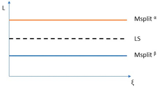
Figure 1.
The idea of Msplit estimation and least-squares estimation.
Figure 1 presents the result of fitting two lines into a dataset of points using the Msplit method and least-squares (LS) method.
According to the assumption of this method, it is also possible to fit two or more planes simultaneously in a dataset. This is due to the theoretical basis of this method. However, this method has a certain limitation, and the functional model must be selected very carefully in terms of the mathematical description of the estimated model and data structure. In the sense of least-squares, the best fit minimizes the sum of the squared distances from observation to model, usually along with the observed variable. So, from a geometric point of view, the residuals are parallel to one of the axes of the coordinate system.
Figure 2 shows the result of fitting the line into a point set by the least-squares method performed in two cases depending on the data distribution.
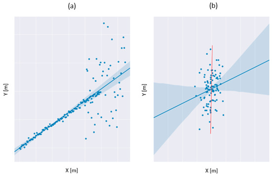
Figure 2.
Correct (a) and incorrect (b) data fitting based on the same functional model depending on the data distribution.
In Figure 2, the color blue (shadow area) indicates the confidence interval for the regression estimate. The confidence interval was drawn using translucent bands around the regression line. The dark blue dots represent the observations in which a straight line fits. Two cases, figure a and figure b, show straight line options depending on the data distribution. In cases where the variance of residuals is almost parallel to the estimator axis (such as in Figure 2b), the results are ambiguous.
2.2. Orthogonal Regression
The least-squares method is classified as a linear regression method, and a statistical procedure is used to find the best fit for a set of data. However, orthogonal regression is also very often used to analyze measurement data. The history of the orthogonal regression method is very long and has been described many times in the statistical literature: [13,14,15,16,17].
The idea of the orthogonal regression is to minimize the sum of the squared orthogonal distances from the data points to the fitting model. The classical least-squares method minimizes the sum of the residuals parallel to one of the axes of the coordinate system from the data point to the fitting, for example, as a line or plane. A detailed and extensive discussion of the method can be found in [18]. The differences between the orthogonal regression (OR) and LS methods are present in Figure 3.
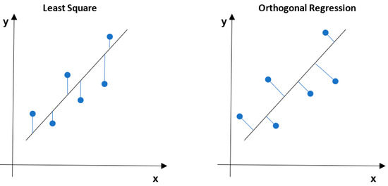
Figure 3.
The graphical comparison between least-squares and orthogonal regression.
As mentioned in the previous section, correct LS data matching based on the same functional model depends mainly on data distribution. This problem does not occur using the orthogonal regression, as shown in Figure 3.
One more modification was introduced in the proposed OMsplit estimation approach, i.e., the objective function is minimized by the Nelder–Mead method. The parameters are not estimated in a direct manner, but instead, the Nelder–Mead method is applied to numerically find the minimum of the objective function.
2.3. Nelder–Mead Simplex Method
The Nelder–Mead method is a numerical method used to find the minimum of an objective function in a multidimensional space. It is a direct search method suitable for nonlinear optimization problems because the algorithm does not use derivatives. It is based only on calculating the objective function’s values [19]. Finally, a structured method tends to a global minimum. A detailed description of the method can be found in [20].
The Nelder–Mead simplex method starts with forming a simplex (set of points) in a multidimensional space. The number of vertices of the simplex is bigger than the parameter space dimension by one. The number of parameters is equal to the dimension of space. For example, a one-dimensional simplex, which is the section of a straight line, has two vertices, whereas a two-dimensional simplex has three vertices, so it is a triangle. Generally, the n-dimensional simplex of the n + 1 vertices is a polyhedron represented by n + 1 vectors.
The first step is to form the initial simplex, assuming a distance between the vertices. Usually, the default is five percent of the parameter value. The next step is a transformation of the simplex as long as the distance between the vertices is less than the assumed accuracy of the calculations. During optimization, the simplex procedure is modified many times until it reaches the global minimum. In searching for the minimum objective function, the following operations are applied: calculating the center of gravity of the simplex, reflection, expansion, contraction, and reduction [20].
The Nelder–Mead method was introduced to the presented solution of orthogonal Msplit estimation due to it being less time and resource consuming. Moreover, it is more robust to the local minimum of the objective function than the LS method.
2.4. Processing with Orthogonal Msplit Estimation
A plane in three-dimensional space can be described by the following standard form of the plane equation:
where the following are defined:
A, B, C, D—plane parameters;
x, y, z—coordinates;
di—the distance of a single point from the plane, calculated as:
The weighted sum of the squares of point to plane distances was assumed as an objective function:
where wi denotes the weight of the i-th point and the distance from the plane to point (x,y,z) can be expressed as:
Next, the Nelder–Mead method is used to find A, B, C, and D parameters for which the objective function value is the minimum. Thus, the search for parameters is not strictly carried out, but the selected Nelder–Mead method is conducted numerically. In the OMsplit estimation process, the parameters of two planes, α and β, are estimated. To achieve this task, the cross-weighting procedure is carried out. The first step is called alpha solution (“1”). The alpha residuals are calculated based on the alpha parameters (“2”). Then, the beta weights (pβi) of the observation are modified according to Equation (3). The parameters and free terms are updated. In the next step, the second (beta) solution is calculated using the Nelder–Mead method using pβi. The new weights for the α solution are computed with Equation (4). Then, the procedure goes back to the α solution, and the process is iteratively repeated until the increase in estimated parameters reaches a satisfying level.
The procedure is shown in Figure 4. The block diagram presents the modification (marked in red color) in relation to the procedure already described by the authors in the previous article. Numbers from 1 to 7 denote the sequence of calculation operations performed. The implementation of orthogonal regression significantly improves the functioning of the proposed OMsplit estimation method.
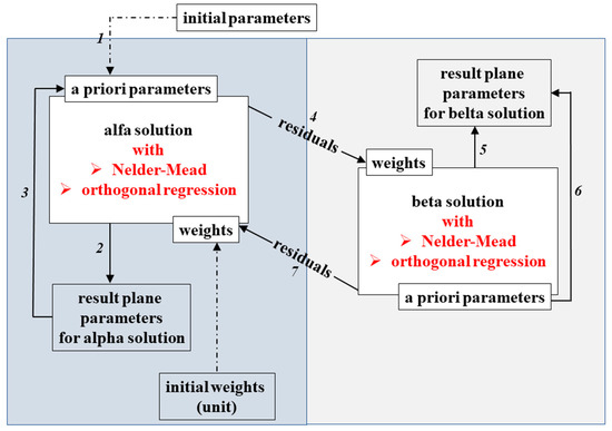
Figure 4.
The block diagram of the orthogonal Msplit estimation.
2.5. Description of Research Objects
The simulated and the real point cloud data were processed using the described method.
The simulated object is represented by two mathematical functions zi = f (x, y), where i = 1,2:
z1 = 7x + 2y − 9.5
z2 = x + 2y +3
The point cloud representing the test object is presented in Figure 5.
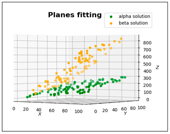
Figure 5.
The point cloud representing the test object.
Thus, two data sets of points were obtained, and during the next step, they were combined into one simulated set. This approach allows one to formulate the assumption that after using OMsplit, the user should obtain two fitted planes into two initial point clouds.
The real object was a fragment of a retaining wall near the Primary School in Olsztyn, which was damaged after a violent storm. Part of the wall was moved due to a large amount of rainwater, causing a landslide. Because of the landslide, the concrete slabs that make up this wall and protect the area changed their position. Individual concrete slabs parted to the side, a gap formed between them, and the inclination angle changed.
The considered real object (two plates with the most significant displacement) is shown in Figure 6.
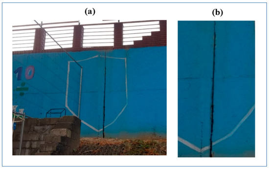
Figure 6.
The concrete slabs and a gap formed between them after a storm: (a) the fragment of the retaining wall; (b) the fragment of the wall is used to fit the planes.
The measurements were performed using a Leica Scan Station C10 based on two stations, with a distance of about 7 m and a resolution of 2 mm. The point cloud representing the fragment (Figure 6b) of the retaining wall is presented in Figure 7a.
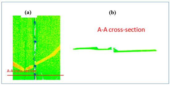
Figure 7.
The point cloud representing the fragment of the retaining wall: (a) front view, (b) cross-section.
The obtained point cloud was processed using the OMsplit estimation method. Two functional models were established during the processing corresponding to the points depicting a particular concrete slab. The results are presented and discussed in the next point.
3. Results
According to the algorithm presented on the block diagram, calculations were performed on the test sets and on the real data obtained as a result of measurement with a terrestrial laser scanner.
In previous studies [21], the authors tested the Msplit estimation method in the context of detecting and dimensioning displacements of adjacent planes on several real datasets with different numbers of points. The solution presented in this paper is an extension of previous research by introducing orthogonal regression to the computational process.
The authors present the results of the introduced improvement on one test set and one real set. The obtained results are presented and described in this section.
3.1. Simulated Objects Results
Figure 8 shows the result of the automatic fitting of two planes to the point cloud using the OMsplit method.
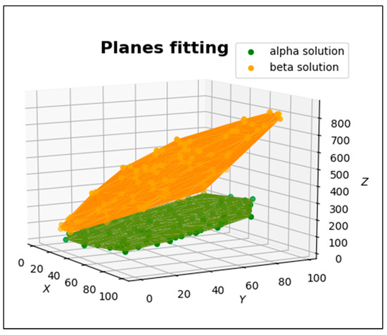
Figure 8.
The result of the simulated fit of the two planes.
Figure 9 presents the characteristics of the residuals obtained for each solution: alpha and beta. The “residual values” graph presents the distribution of the residuals for the alpha and beta solutions. It can be observed that the residuals from point numbers 1–10 (Figure 9a green color) are close to 0 m, while the residuals marked in orange are in the range of point numbers 1–10 and are about 20 to 50 m. The opposite situation is seen in the range of point numbers 10–20. This means that points 1–10 have been assigned to the alpha plane, and points 10–20 have been assigned to the beta plane.
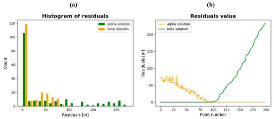
Figure 9.
(a) The histogram of the residuals; (b) the residual for α and β solutions.
3.2. Real Object Results
The obtained point cloud was processed using the new orthogonal Msplit estimation method. Two functional models were established during the processing corresponding to the points depicting a particular concrete slab. The fitting results are presented in Figure 10.
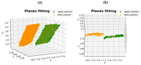
Figure 10.
The results of the real object-fit ((a) front view; (b) top view).
Analyzing Figure 10, it can be observed that the point cloud was correctly divided into two planes.
In Figure 11a histogram of residuals and residuals values are presented.
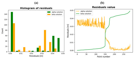
Figure 11.
(a) The histogram of the residuals; (b) the residual for α and β solutions.
Based on the “residual values” graph in Figure 11b, it can be observed that the residuals from point number 1 to point number 151 (green color) do not exceed 0.01 m, while the residuals marked in orange in the range of point numbers 1–151 are about 0.04 m.
The opposite situation is in the range of point numbers 151 to 285. This means that points 1–151 have been assigned to the alpha plane, and points 151–285 have been assigned to the beta plane.
Root-mean-square (RMS) values were calculated for each plane fitting (Table 1). In each case, the RMS value for both the α and β solutions are similar, concluding that the two planes in each object were extracted and that no other planes or outliers are present in the point cloud. The distribution of points relative to the fitted planes in each of the two presented objects is even. Table 1 shows the plane parameters received for real objects in the α and β solutions, the number of points assigned to each plane, and the RMS values for the alpha and beta solutions.

Table 1.
Numerical characteristics.
4. Discussion
This paper applied the orthogonal Msplit estimation method used to automatically fit two planes into one point cloud. The proposed method can be used if mathematical algorithms and functions can describe an object or its elements. The inspiration was a real situation that recently occurred after heavy rain. Rainwater flooded the ground, resulting in a retaining wall being moved. The concrete slabs constituting the elements of the wall were displaced in relation to each other. One option was to measure this wall using a terrestrial laser scanner to estimate the extent of the damage.
As a result of TLS measurement, the dataset is usually composed of one point cloud (or scans registered into one cloud). In the previous paper, the authors proposed using the Msplit estimation method for this purpose. The efficacy of the Msplit method has been confirmed by tests carried out on different datasets. However, despite its effectiveness, the Msplit estimation method has a particular disadvantage. When using the proposed method, it should be remembered that functional models should be appropriately formulated depending on whether they are of horizontal or vertical planes. A functional model must be selected carefully and based on a mathematical description of the estimated model and data structure. It is necessary to formulate a model matching the data or to match the data to the model every time. As a result, using Msplit estimation for LIDAR data is not a universal solution. The solution to this problem is the orthogonal Msplit estimation method proposed by the authors in this manuscript. The introduced improvements, the orthogonal regression and Nelder–Mead method, allow the solution to achieve universality, regardless of how the functional model is formulated. The conducted tests confirmed the correctness of the introduced modifications, and the content of this article describes the applied approach.
Further work related to the development of the proposed OMsplit estimation method will be related to rewriting the developed algorithm to a more efficient programming language. The authors used the Python programming language for the calculations in this paper; however, it is not an efficient programming language, which also forced the authors to reduce the size of the original dataset of the real object before performing the plane fitting.
In addition to the limited efficiency of the programming language used by the authors, there is also the issue of the sensitivity of the proposed method. The size of the displacement is an important issue here. To split the functional model into at least two models, these models must be described by different parameters. This means that the planes must be distinguishable in a point cloud measured with TLS. However, the situation can also be interpreted so that if they do not split the model into two (or more, depending on the situation), it can be said that there was no displacement.
5. Conclusions
The orthogonal Msplit (OMsplit) estimation can be successfully applied in the detection of two planes. The method allows one to correctly separate a dataset into two and fit each plane to the appropriate dataset. In the solution proposed by the authors, the sum of the squared orthogonal distances from the data points to the fitting line is minimized. Therefore, it has a big impact on the universality of this solution.
The application of the described solution does not require additional actions; i.e., there is no need to properly prepare the data or the model.
Author Contributions
Conceptualization, J.J. and J.R.; methodology, J.J. and J.R.; software, J.R.; investigation, J.J.; resources, J.J. and J.R.; data curation, J.J.; writing—original draft preparation, J.J. and W.B.-B.; writing—review and editing, W.B.-B.; visualization, J.J. All authors have read and agreed to the published version of the manuscript.
Funding
This research received no external funding.
Data Availability Statement
Data available on request due to restrictions privacy.
Conflicts of Interest
The authors declare no conflict of interest.
References
- Axelsson, P. Processing of laser scanner data—Algorithms and applications. ISPRS J. Photogramm. Remote Sens. 1999, 54, 138–147. [Google Scholar] [CrossRef]
- Wang, C.; Hsu, P. Building detection and structure line extraction from airborne lidar data. J. Photogramm. Remote Sens. 2007, 12, 365–379. [Google Scholar] [CrossRef]
- Zheng, J.; Mc Carthy, T.; Fotheringham, A.S.; Yan, L. Linear feature extraction of buildings from terrestrial LIDAR data with morphological techniques. Int. Arch. Photogramm. Remote Sens. Spat. Inf. Sci. 2008, 37, 241–244. [Google Scholar]
- Diab, A.; Kashef, R.; Shaker, A. Deep Learning for LiDAR Point Cloud Classification in Remote Sensing. Sensors 2022, 22, 7868. [Google Scholar] [CrossRef] [PubMed]
- Nahhas, F.H.; Shafri, H.Z.M.; Sameen, M.I.; Pradhan, B.; Mansor, S. Deep Learning Approach for Building Detection Using LiDAR–Orthophoto Fusion. J. Sensors 2018, 2018, 1–12. [Google Scholar] [CrossRef]
- Soilán, M.; Riveiro, B.; Balado, J.; Arias, P. Comparison of heuristic and deep learning-based methods for ground classifi-cation from aerial point clouds. Int. J. Digit. Earth 2020, 13, 1115–1134. [Google Scholar] [CrossRef]
- Liu, B.; Huang, H.; Su, Y.; Chen, S.; Li, Z.; Chen, E.; Tian, X. Tree Species Classification Using Ground-Based LiDAR Data by Various Point Cloud Deep Learning Methods. Remote Sens. 2022, 14, 5733. [Google Scholar] [CrossRef]
- Zhang, L.; Wang, J.; Shen, Y.; Liang, J.; Chen, Y.; Chen, L.; Zhou, M. A Deep Learning Based Method for Railway Overhead Wire Reconstruction from Airborne LiDAR Data. Remote Sens. 2022, 14, 5272. [Google Scholar] [CrossRef]
- Janowski, A.; Rapinski, J. M-Split Estimation in Laser Scanning Data Modeling. J. Indian Soc. Remote Sens. 2012, 41, 15–19. [Google Scholar] [CrossRef]
- Wiśniewski, Z. Split Estimation of Parameters in Functional Geodetic Models. Tech. Sci. 2008, 11, 202–212. [Google Scholar] [CrossRef]
- Wiśniewski, Z. Estimation of parameters in a split functional model of geodetic observations (M split estimation). J. Geodesy 2008, 83, 105–120. [Google Scholar] [CrossRef]
- Wiśniewski, Z. M split(q) estimation: Estimation of parameters in a multi split functional model of geodetic observations. J. Geodesy 2010, 84, 355–372. [Google Scholar] [CrossRef]
- Adcock, J. Note on the method of least squares. Analyst 1877, 4, 183–184. [Google Scholar] [CrossRef]
- Pearson, K. On lines and planes of closest fit to systems of points in space. Philos. Mag. J. Sci. 1901, 2, 559–572. [Google Scholar] [CrossRef]
- Koopmans, T.C.; Hood, W.C. (Eds.) The estimation of simultaneous linear economic relationships. In Studies in Econometric Method; John Wiley: New York, NY, USA, 1953. [Google Scholar]
- Madansky, A. The Fitting of Straight Lines When Both Variables Are Subject to Error. J. Am. Stat. Assoc. 1959, 54, 173–205. [Google Scholar] [CrossRef]
- Golub, G.H.; Van Loan, C.F. An Analysis of the Total Least Squares Problem. SIAM J. Numer. Anal. 1980, 17, 883–893. [Google Scholar] [CrossRef]
- Markovsky, I.; Van Huffel, S. Overview of total least-squares methods. Signal Process. 2007, 87, 2283–2302. [Google Scholar] [CrossRef]
- Kozieł, S.; Yang, X.S. Computational, optimization, methods and algorithms. In Studies Is Computational Intelligence; Springer: Berlin/Heidelberg, Germany, 2011; Volume 356. [Google Scholar]
- Nelder, J.A.; Mead, R. A Simplex Method for Function Minimization. Comput. J. 1965, 7, 308–313. [Google Scholar] [CrossRef]
- Janicka, J.; Rapiński, J.; Błaszczak-Bąk, W.; Suchocki, C. Application of the Msplit Estimation Method in the Detection and Dimensioning of the Displacement of Adjacent Planes. Remote Sens. 2020, 12, 3203. [Google Scholar] [CrossRef]


Disclaimer/Publisher’s Note: The statements, opinions and data contained in all publications are solely those of the individual author(s) and contributor(s) and not of MDPI and/or the editor(s). MDPI and/or the editor(s) disclaim responsibility for any injury to people or property resulting from any ideas, methods, instructions or products referred to in the content. |
© 2023 by the authors. Licensee MDPI, Basel, Switzerland. This article is an open access article distributed under the terms and conditions of the Creative Commons Attribution (CC BY) license (https://creativecommons.org/licenses/by/4.0/).