1. Introduction
Earth rotation parameters (ERPs) are the key conversion parameters connecting the international terrestrial reference frame (ITRF) and international celestial reference frame (ICRF) and can be divided into two parts: (1) those that describe variations in the Earth’s rotation rate, i.e., universal time (UT1-UTC) or length of day (LOD); (2) and those that monitor variations in the position of the Earth’s axis, i.e., polar motion (PMX, PMY) [
1,
2]. With the rapid development of space geodetic techniques, more techniques are being applied to monitor variations in the Earth’s rotation, such as the global navigation satellite system (GNSS (Toulouse, France)), very long baseline interferometry (VLBI (National Astronomical Observatory of Japan, Tokyo, Japan)), satellite laser ranging (SLR), lunar laser ranging (LLR), and doppler orbitography and radio positioning integrated by satellite (DORIS) [
3,
4,
5].
The Earth’s rotation not only represents the state of its overall movement, but also reflects the interactions and mechanical processes between the solid earth and the atmosphere, ocean, mantle, and crust on the temporal and spatial scale [
6]. Therefore, variations in ERPs indicate variations in various geophysical factors. The highly accurate determination and estimation of ERPs with high precision and resolution has great reference value for exploring not only the activities of the Earth, Sun, and Moon, but also can explore the law of material movement in the Earth’s interior [
7,
8]. The research on ERP estimation has been conducted by many scholars mainly based on GNSS, VLBI, SLR, and other techniques. For polar motion estimation, the results of this study indicate that GNSS occasionally has superior accuracy, which is due to the large number of International GNSS Service (IGS) stations homogeneously distributed around the globe, as discovered by Dow and Neilan [
9]. Böhm et al. [
8] proposed a method, operated in time domain, that is easily applicable to ERP estimation from VLBI. Accurate UT1-UTC results allow detailed studies of geodynamic phenomena and probing of excitations [
10]. Brzezinski et al. [
11] reported that diurnal and semi-diurnal atmospheric effects on ERP, polar motion, and variations in LOD were below 10 μas and 10 μs, respectively. In addition, the International VLBI Service for Geodesy and Astrometry (IVS) has organized a 2-week continuous VLBI campaign (CONT) every third year since 2002 [
12]. The observations from these campaigns have been used in many studies with different objectives, comparing the accuracy of GNSS and VLBI to estimate Earth orientation parameters (EOP) [
13]. Using CONT17 observations, Puente [
14] compared the accuracy of GNSS- and VLBI-estimated troposphere, station coordinates, zenith total delays (ZTDs), and gradients.
The demand for real-time ERPs is growing due to space navigation and positioning; however, obtaining real-time ERP is more difficult due to the complex data processing [
15]; for example, GPS processing takes about 3 h, while VLBI and SLR take longer to process. Various prediction methods are applied in ERP research.
Table 1 indicates the prediction accuracy of the latest PM and UT1-UTC over various spans provided by the IERS (IERS Rapid Service/Prediction Centre). Based on least squares (LS), Kosek et al. [
16] proposed a combined LS and autoregressive (AR) model for ERP prediction. Atmospheric angular momentum (AAM) prediction data are considered to be beneficial to improve the forecast accuracy of UT1 and LOD [
4]. Schuh et al. [
17] reported on incorporating artificial neural networks (ANN) into PM and UT1-UTC predictions. Furthermore, fuzzy inference system [
15], multi-channel singular spectrum analysis (MSSA) [
18], neural ordinary differential equations (ODE) differential learning [
19], and fuzzy-wavelet [
20] have been applied to ERP prediction.
Regarding the possible causes of ERP prediction errors, the effect of El Niño on the prediction of polar motion must be taken into account [
21]. Considering the axial component of atmospheric angular momentum (AAM
X3), a combined multivariate autoregressive (MAR) model forecasting method was proposed by Niedzielski [
22]. Chin et al. [
23] investigated the short-term prediction of the polar motion by introducing a prediction model with an excitation function. It involved incorporating integrations of AAM estimates into UT1 series, as reported in a study by Gambis [
24]. Long-term predictions of polar motion take into account the instantaneous frequency, phase, and amplitude of the Chandler motions, prograde, and retrograde annual motions of the Earth, and also the normal wavelet transform (NTFT), as reported by Su [
25].
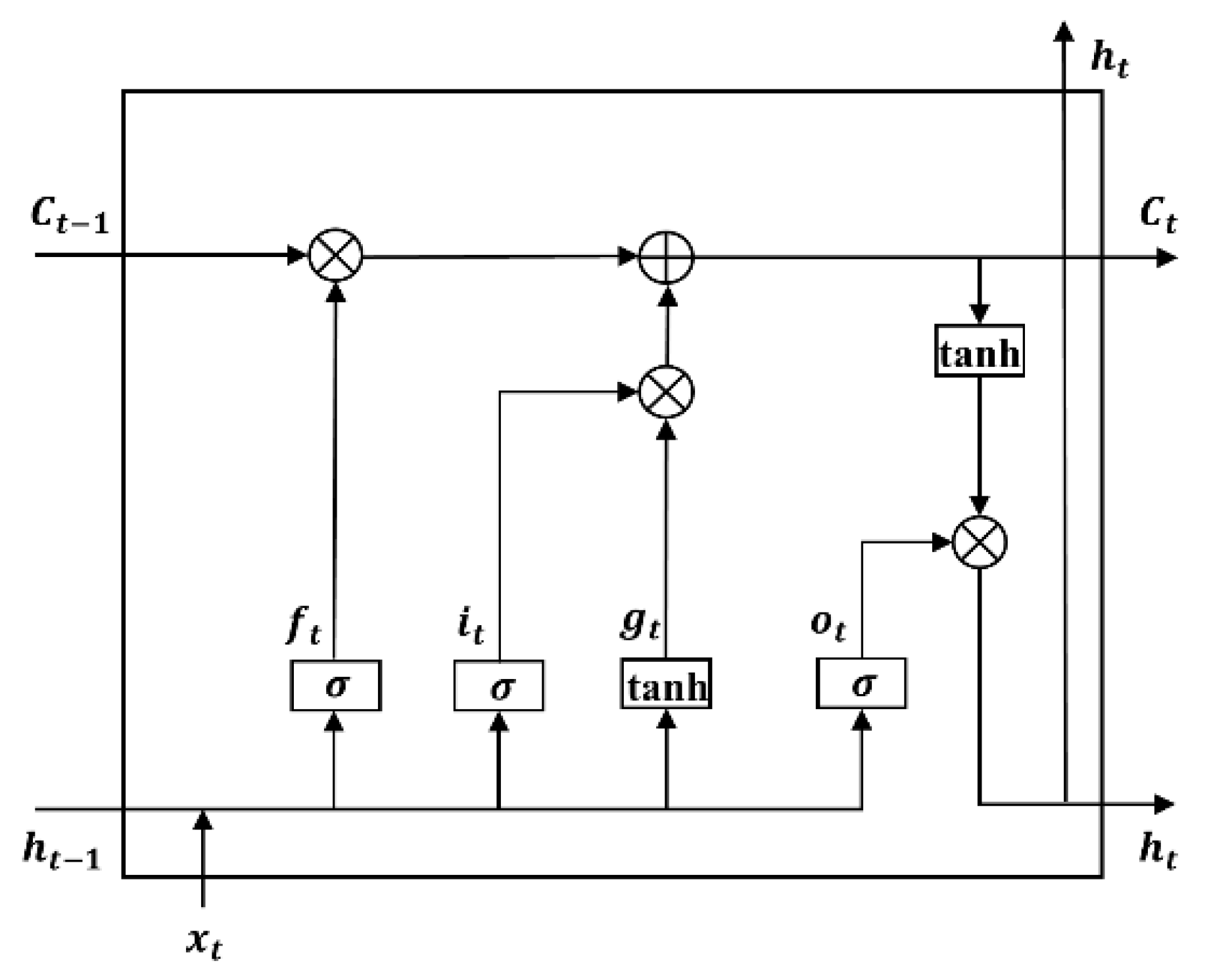
In addition, hybrid neural networks, which have drawn more attention recently, combine the advantages of different neural networks. Several previous studies combined convolutional neural networks and long short-term memory (CNN–LSTM) to address temporal and spatial relations, respectively [
26]. CNN can extract and optimize trend features for different time series [
27], while LSTM is specifically designed to make long-term predictions based on historical time series [
28]. Augmenting fully CNN–LSTM sub-modules for time series classification was proposed by Karim [
29]. An attention-based CNN–LSTM model to predict collaborations between different research institutions was reported by Zhou [
30].
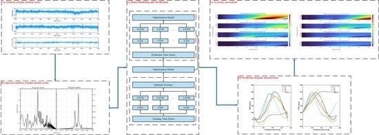
The aim of this paper was to estimate ERP based on VLBI observations from 2011 to 2020 and predict polar motion series based on the hybrid CNN–LSTM model, the experiments of this paper can be described as follows:
VLBI observations from 2011 to 2020 were estimated by Vienna VLBI Software 3.2 (VieVS 3.2) [
31,
32] to obtain 10-year ERP time series. Furthermore, in order to compare the difference in ERP accuracy between other VLBI solutions, we estimated the observations of the CONT08, CONT11, CONT14, and CONT17 campaigns. To further explore high-frequency variations and investigate long-term series information of polar motion, fast Fourier transform (FFT) was used for the spectral analysis of polar motion series;
The LS + AR model is currently one of the more accurate models for short-term polar motion series prediction; however, it is less effective in medium- and long-term prediction. This experiment aims to resolve the problem that the existing methods are not effective for the medium- and long-term prediction of polar motion series and the inadequate modelling capabilities of various influencing factors. In this paper, a hybrid CNN–LSTM model to predict polar motion is proposed by this paper; the CNN model can effectively extract features that affect polar motion series, and the LSTM model has natural advantages in the medium- and long-term time series prediction. To compare the differences in prediction accuracy, we also construct the LS + AR models for polar motion prediction based on Earth orientation parameters prediction comparison campaign (EOP PCC) [
1,
33].
4. Discussion
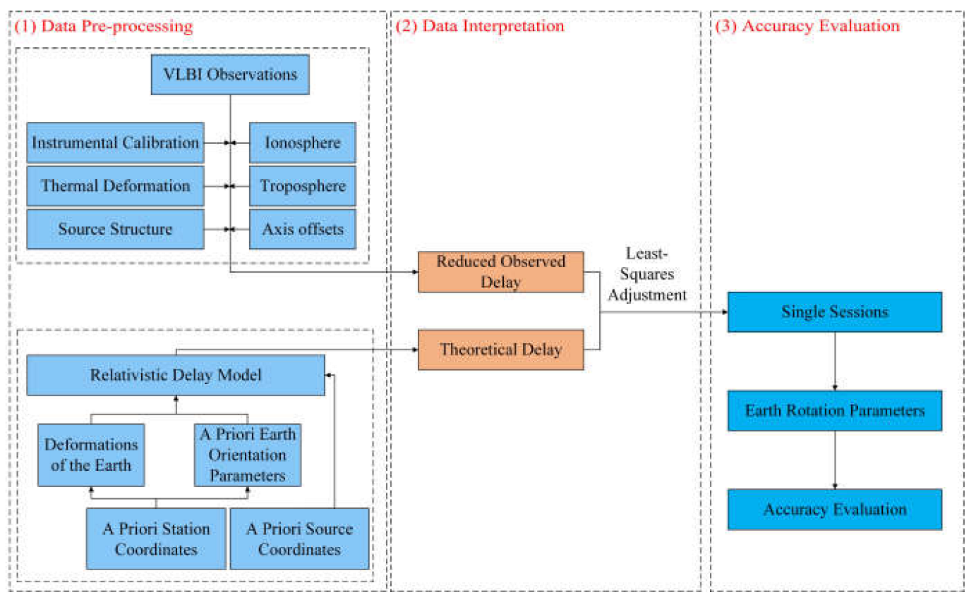
The International VLBI Service for Geodesy and Astrometry (IVS) organized IVS-R1 and IVS-R4 sessions every Monday and Thursday, respectively, and these sessions usually involve a network of 5–10 VLBI stations for observation [
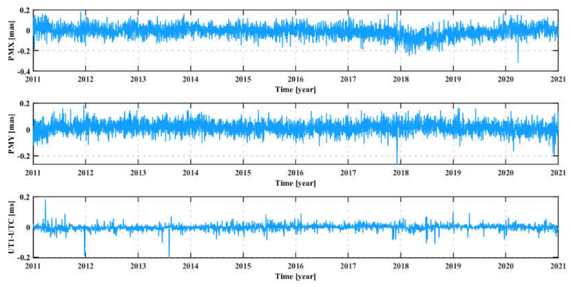
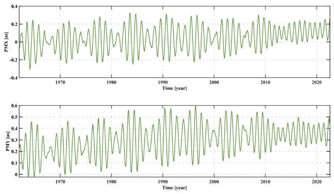
13]. In this paper, the ERP series were obtained by estimating VLBI observations from 2011 to 2020 for IVS-R1/R4 sessions; furthermore, the CONT08, CONT11, CONT14, and CONT17 observations were estimated. The results show that the average RMSE based on the IVS-R1/R4 solution is about 0.19 mas for polar motion and 0.02 ms for UT1-UTC, while the accuracy of the CONT solutions is about 0.04 mas and 0.01 ms for polar motion and UT1-UTC, respectively. There may be two reasons for these results: One may be that the IVS-R1/R4 sessions have only 5–10 stations, while CONT campaigns have more globally distributed stations, and the IVS-R1/R4 sessions have a lower rate of data recording (256 Mbit/s) rather than the faster 512 Mbit/s. Another reason may be the difference in accuracy due to the epoch continuum.
Obviously, polar motion is one of the key parameters of ERP, which is defined as the motion of the Celestial Intermediate Pole (CIP) relative to the Earth’s surface. It is composed of a collection of motions covering a range from secular to sub-daily time scales [
50]. The polar motion series consists of three significant components: long-term trend, Chandler wobble, and annual wobble. The large-scale secular deformation of Earth causes long-term drift of the polar motion [
51]. The Chandler wobble refers to the motion of the CIP over the Earth’s surface, which is caused by the rotation axis not being aligned with the inertia axis [
50], and is an excited resonance of the Earth’s rotation over a period of about 14 months [
52]. The annual wobble is another important component of the polar motion and current findings confirm that it consists of two components, retrograde, and prograde wobble [
53,
54].
Furthermore, to explore the high-frequency variations in more detail, fast Fourier transform (FFT), for polar motion time series spectrum analysis, was selected in this paper. The spectrum of polar motion series is plotted in
Figure 7, and the results show that the polar motion series exhibit extremely significant Chandler and annual wobble of about 426 days and 360 days, respectively. In addition, the results also showed a weaker retrograde oscillation with an amplitude of about 3.5 mas, and we enlarged the scale of the amplitude in order to explore more details of the retrograde wobble. Previous studies have proposed that the possible causes of excitation for Chandler wobble include variations in submarine, atmospheric, and groundwater pressure, as well as seismic excitation, and the annual wobble may be excited by variations in the atmosphere, ocean, and groundwater [
55,
56,
57].
Moreover, a hybrid CNN–LSTM model is proposed in this paper, which is used for polar motion time series of prediction.
Table 6 shows the comparison of the MAE of Bulletin A and the 12-year polar motion prediction based on the hybrid CNN–LSTM model. Compared with Bulletin A, the results show that the accuracy of the hybrid CNN–LSTM model is slightly inferior in ultra-short-term polar motion prediction; this is because the model is being trained in the initial stage when it is less effective. However, the prediction accuracy gradually improved over time; notably, the prediction accuracy for PMX and PMY over a time span of 360 days improved by 42% and 13%, respectively. These results support the conclusion that the hybrid CNN–LSTM model can indeed improve the prediction accuracy of polar motion.
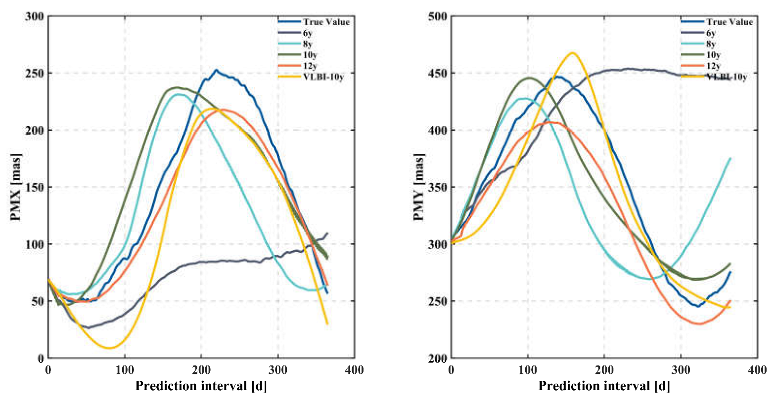
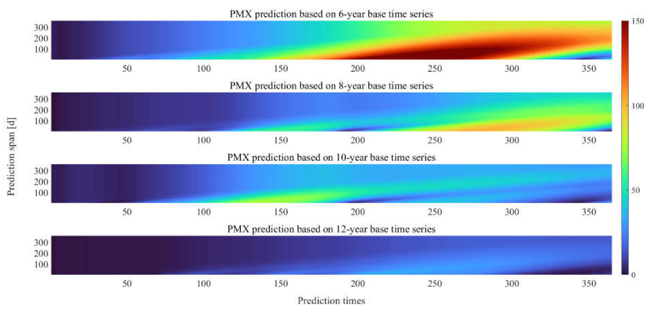
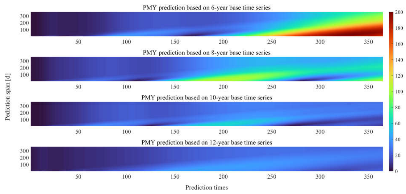
Figure 8 and
Figure 9 show the mean absolute error (MAE) of 360-day polar motion prediction using the EOP 14C04 series for the period 1 January 2009 to 31 December 2020. PMX and PMY with 6-year base time series show large errors, especially for medium- to long-term prediction (180–360 days), which is mainly due to the poor training effect caused by the short time series. At the same time, we found that the 12-year base time series had the highest prediction accuracy, mainly due to the fact that the prediction accuracy can be optimized when the length of the base time series is sufficient.
5. Conclusions
Earth rotation parameters play a crucial role in high-precision timing services, precise orbiting of artificial satellites, etc. Prior studies have noted the importance of estimating and predicting ERP. We obtained the ERP series by estimating VLBI observations from 2011 to 2020 for IVS-R1/R4 sessions; furthermore, the CONT08, CONT11, CONT14, and CONT17 observations were estimated. The results show an average RMSE of 0.187 and 0.205 mas for PMX and PMY, respectively, and accuracy of 0.022 ms for UT1-UTC based on IVS-R1/R4 solutions. The accuracy of polar motion for CONT solutions was in the range of 0.03–0.05 mas, and for UT1-UTC based on the CONT solutions it was 0.005–0.01 ms.
Furthermore, to investigate the high-frequency variations in more detail, we performed spectral analysis of the polar motion series using fast Fourier transform (FFT). The results show that the polar motion series exhibit extremely significant Chandler and annual wobble of about 426 days and 360 days, respectively. In addition, the results also show weaker retrograde oscillation with an amplitude of about 3.5 mas.
Another important finding is that the hybrid CNN–LSTM model proposed in this paper is applicable to polar motion prediction. In short term prediction (0–60 days), the LS + AR model was superior, whereas in medium- to long-term prediction (90–360 days), the hybrid CNN–LSTM model improved PMX and PMY 54% and 31%, respectively. These results further support the observation that the hybrid CNN–LSTM model is slightly less accurate in short-term prediction and more accurate in medium- and long-term prediction. One possible explanation for these results is that the model may not have been trained optimally at the beginning. In addition, possible interference of the base time series cannot be ruled out. We tested the variability of the effect of different base series on the prediction of polar motion, and the results indicate that the accuracy of the prediction model gradually improved over time.
One limitation of the methods in this paper is that the training model for the 6-year base series was not very effective, and this needs to be further explored in our next work. We also need to consider the effect of numerous excitation sources on the prediction accuracy. Our future work will be devoted to investigating the effect of different excitation sources and base time series on prediction accuracy.


