Article

Mapping Population Distribution with High Spatiotemporal Resolution in Beijing Using Baidu Heat Map Data

1
State Key Laboratory of Remote Sensing Science, Beijing Normal University, Beijing 100875, China
2
Beijing Key Laboratory of Environmental Remote Sensing and Digital City, Beijing Normal University, Beijing 100875, China
3
Key Laboratory of Environmental Change and Natural Disaster, MOE, Beijing Normal University, Beijing 100875, China
4
State Key Laboratory of Earth Surface Processes and Resource Ecology, Beijing Normal University, Beijing 100875, China
5
School of Statistics, Beijing Normal University, Beijing 100875, China
*
Author to whom correspondence should be addressed.
Remote Sens. 2023, 15(2), 458; https://doi.org/10.3390/rs15020458
Submission received: 21 December 2022 / Revised: 7 January 2023 / Accepted: 8 January 2023 / Published: 12 January 2023

Abstract

:
Population distribution data with high spatiotemporal resolution are of significant value and fundamental to many application areas, such as public health, urban planning, environmental change, and disaster management. However, such data are still not widely available due to the limited knowledge of complex human activity patterns. The emergence of location-based service big data provides additional opportunities to solve this problem. In this study, we integrated ambient population data, nighttime light data, and building volume data; innovatively proposed a spatial downscaling framework for Baidu heat map data during work time and sleep time; and mapped the population distribution with high spatiotemporal resolution (i.e., hourly, 100 m) in Beijing. Finally, we validated the generated population distribution maps with high spatiotemporal resolution using the highest-quality validation data (i.e., mobile signaling data). The relevant results indicate that our proposed spatial downscaling framework for both work time and sleep time has high accuracy, that the distribution of the population in Beijing on a regular weekday shows “centripetal centralization at daytime, centrifugal dispersion at night” spatiotemporal variation characteristics, that the interaction between the purpose of residents’ activities and the spatial functional differences leads to the spatiotemporal evolution of the population distribution, and that China’s “surgical control and dynamic zero COVID-19” epidemic policy was strongly implemented. In addition, our proposed spatial downscaling framework can be transferred to other regions, which is of value for governmental emergency measures and for studies about human risks to environmental issues.

1. Introduction

Rapid urbanization worldwide has not only led to an increase in impervious surfaces but also has been accompanied by an influx of people into cities seeking more employment opportunities and better living benefits [1,2,3]. Therefore, the influx of population poses new challenges for urban planning and environmental issues such as unbalanced regional growth, hazard responses, water resource shortages, severe traffic congestion, and carbon-induced air pollution, particularly in internationally linked metropolises such as Beijing [4,5]. Meanwhile, since the outbreak of COVID-19 in late 2019, recurrent outbreaks have occurred due to high population densities and frequent population movements in metropolitan areas [6,7,8]. Therefore, understanding highly accurate population distribution information with high spatiotemporal resolution is of great significance for environmental change, urban development planning, disaster assessment management, and epidemic prevention and control [9,10,11,12,13,14].
Over the past few decades, a number of approaches, such as simple spatial interpolation, dasymetric-based linear statistical models and machine learning models, have been developed to downscale census data to grid cells from global to local scales by using multi-source ancillary data [15,16,17,18,19,20,21,22,23,24]. Dasymetric mapping has proven to be an effective spatial downscaling method and is widely used to generate gridded population density maps. Its core idea is to generate weight layers based on ancillary data and use the weight layers to disaggregate coarse resolution variables (e.g., population) to a finer resolution [10,25,26]. Widely used ancillary data are satellite-based remote sensing products [27], such as nighttime light (NTL) images [28,29,30] and land use/land cover (LULC) [31,32,33]. In recent years, emerging geospatial big data, such as point of interest (POI) data and building volume data, have also been used as ancillary data to disaggregate census data, which provides new opportunities for generating more accurate gridded population density maps [34,35,36,37,38]. In addition, there are many high-quality and freely available global gridded population density maps, such as the LandScan global population database (1 km) [39,40] and WorldPop global population product (100 m) [41], which are also produced by dasymetric mapping in combination with multi-source ancillary data. However, population is a temporally dynamic variable, with major shifts in its distribution occurring in daily cycles, resulting in rapidly changing densities [42]. Therefore, these products are limited in terms of their temporal resolution and cannot accurately represent the dynamic distribution of the population. In addition, although commonly used ancillary data can successfully allocate census data into space, the static nature of the input dataset obscures the specific time at which the population distribution refers [43,44]. Therefore, more dynamic data sources are needed to reflect the short-term and time-specific spatial redistribution of the population caused by human mobility.
Recently, the rapid development of mobile devices and the enrichment of location-based service (LBS) big data have enabled researchers to analyze human mobility patterns and map population spatial distributions at a finer temporal resolution [45,46,47]. Currently, Baidu heat map data and mobile signaling data are the most popular among dynamic LBS data and possess precise spatiotemporal information, which can be used to study the dynamic distribution of populations and improve the temporal resolution of gridded population density maps [48,49,50]. For both types of data, mobile signaling data is the most promising data source for spatiotemporal populations because it has an extremely high penetration rate across the globe [42,45]. According to statistics, in developed countries, the number of mobile phone subscribers has surpassed the total population, with a penetration rate now reaching 121%, whereas in developing countries, it is as high as 90% and continuing to rise [51]. However, with the current legal frameworks, operators are reluctant to release their data because of privacy issues and a lack of business models [42]. Therefore, the acquisition of such a dataset is still limited in geographic coverage, so it is still difficult to map short-term populations in large areas. Baidu heat map data are widely used in population mobility pattern research because they are publicly available and also have a high penetration rate, which gives the possibility of mapping dynamic population distributions on a large regional scale [52]. However, the highest spatial resolution of the Baidu heat map data currently available is 500 m at the urban scale, which is insufficient to capture subtle population density changes within a city. Therefore, it is crucial to develop a spatial downscaling method for Baidu heat map data to map the population distribution with high spatiotemporal resolution.
POI is a typical kind of geospatial big data. Apart from exact location information, each single POI contains a short textual description to define the category to which the POI belongs. Different categories of POI (e.g., office, school, and factory) represent different human activities within and surrounding them and subsequently have different levels of correlation with population density [24]. In addition, POI has been utilized to define urban functional districts and land use types [34,35]. Therefore, population products produced using POI and other ancillary data, such as LandScan and WorldPop, are defined as the ambient population (i.e., each pixel value represents the relative magnitude of the probability of population presence during work time) [40,41,42]. Nighttime light data have been proven to have a strong correlation with the spatial distribution of populations [53,54]. Currently, Luojia 1-01 NTL data is the highest spatial resolution (130 m) NTL data, and according to related research, NTL combined with building volume data can accurately represent the population distribution of sleep time in large areas [1,55,56]. Therefore, these data provide the opportunity to spatially downscale the Baidu heat map data during work time and sleep time, enabling the mapping of population distributions with high spatiotemporal resolution over large regions.
It is important to develop a rigorously validated and efficient spatial downscaling method for Baidu heat map data for mapping population distribution with high spatiotemporal resolution to improve the understanding of the spatiotemporal distribution characteristics and mechanism of the urban population. We thus innovatively proposed a spatial downscaling framework by integrating multi-source datasets and mapped the gridded population density with high spatiotemporal resolution (i.e., hourly, 100 m) in Beijing. This study’s specific objectives are to (1) integrate ambient population data, nighttime light data, and building volume data to spatially downscale the Baidu heat map data for work time and sleep time; (2) validate the population distribution maps with high spatiotemporal resolution using mobile signaling data; (3) explore the temporal evolution and spatial distribution characteristics of the population in Beijing on weekdays; (4) analyze the relationship between population density distribution and land use types at different time periods; and (5) discuss the impact of epidemic prevention and control policy on population mobility during COVID-19.

2. Materials

2.1. Study Area

Beijing (39°26′N–41°03′N, 115°25′E–117°30′E) is the capital of China; it is a world-famous ancient capital and a modern international metropolis (see Figure 1). Beijing is located in the northern part of the North China Plain, and its terrain is high in the northwest and low in the southeast. It is surrounded by mountains in the west, north, and northeast, and the southeast part is a plain. As of 2022, the city has 16 districts with a total area of 16,410 square kilometers, and its population density ranks 13th among all cities in China. In addition, Beijing is divided into multiple zones by ring roads (beltways). According to statistics, 74.6% of the population dwells within the area within the Sixth Ring Road, which accounts for only 13.8% of the area. Beijing is the political, cultural, and commercial center of the country and therefore attracts a large permanent resident population with complex compositions and structures. Because of urban planning, Beijing has functional divisions, and obvious population mobility can be seen during commuting time. Therefore, taking Beijing as the study area can not only illustrate our proposed spatial downscaling framework well but also analyze the spatiotemporal distribution characteristics of population density in metropolitan areas.

2.2. Data and Preprocessing

The main categories of data used are geospatial big data, remote sensing data, population data, validation data, and basic geographic data. Table 1 lists the 10 types of data used in this study. The retrieval and preprocessing of these datasets in this study are described below. To ensure consistency of spatial location, all data in this paper were reprojected to the WGS-1984-UTM-Zone-50N coordinate system.

2.2.1. Baidu Heat Map Data

Baidu is a leading artificial intelligence (AI) company with a strong internet foundation. Baidu personal computer (PC) terminals and mobile terminals account for 94.72% of the search engine market share, covering 1 billion Chinese users, and the daily response reaches 1300 billion times. In 2011, Baidu Inc. launched a big data visualization product (i.e., Baidu heat map). As a big data application with hundreds of millions of users, the Baidu heat map is based on the location information from users when they access Baidu products (e.g., Baidu Maps, Baidu Search, Baidu Music, Baidu Translate, etc.), which calculates the calorific value of human flow at different times and in different areas and is visualized on Baidu Maps after density analysis processing [48,57]. Therefore, the Baidu heat map can greatly reflect the heat of the crowd in the exact area and is widely used in the study of population dynamic distribution [58].
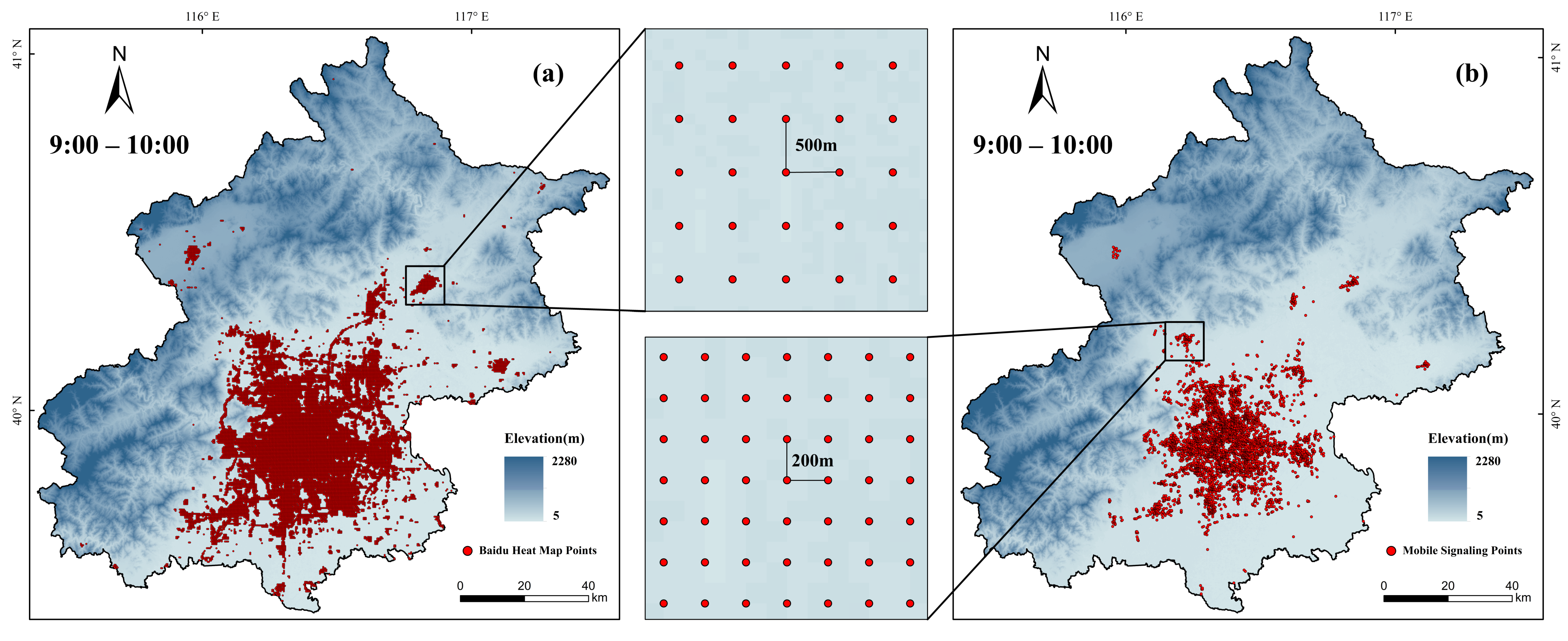
The Baidu heat map data were derived from Baidu Maps (http://map.baidu.com (accessed on 17 August 2022)). We used Baidu’s application programming interface to obtain Baidu heat map data for a total of 24 time periods (0:00–1:00, etc.) in Beijing on 17 August 2022 (Wednesday), with a spatial resolution of 500 m (see Figure 2a). The heat value of each vector point represents the total number of Baidu signal responses for the time period to which it belongs and the spatial range to which it belongs. First, a fishnet with empty attributes at the 500 m × 500 m cell size covering all of Beijing was created in ArcGIS 10.6. Then, we assigned the heat value of each vector point to the corresponding fishnet. Finally, we generated 24 raster layers with a spatial resolution of 500 m using the fishnet with heat value information, corresponding to the 24 time periods. It should be noted that the data we obtained have no personal privacy issues.

2.2.2. Mobile Signaling Data

According to the public data of China’s three major operators, China has a total of 1.619 billion mobile phone users. As of 2022, China has a total of 1.4 billion people, with an average of 1.16 mobile phones per person; thus, the penetration rate of mobile phones in China is extremely high. Mobile signaling data are based on the interaction between mobile phone users and base stations to determine the spatial location of users at different times and will always generate mobile signaling data as long as the phone is on [45]. Therefore, mobile signaling data are the most ideal data source to study population mobility patterns. However, the difficulty of obtaining mobile signaling data makes it difficult to use it to map dynamic population distributions over large areas.
Fortunately, we obtained mobile signaling data from the operators China Mobile, China Unicom, and China Telecom for four time periods (i.e., 0:00–1:00, 9:00–10:00, 15:00–16:00, and 21:00–22:00) in Beijing on 17 August 2022, with a spatial resolution of 200 m and without personal privacy issues (see Figure 2b). However, since the operators provided data for only 5172 geographical points, we used only these data to validate our spatial downscaling framework. The signaling value of each vector point represents the total number of mobile signaling responses for the time period and the spatial range to which it belongs. First, a fishnet with empty attributes at the 200 m × 200 m cell size covering all of Beijing was created in ArcGIS 10.6. Then, we assigned the signaling value of each vector point to the corresponding fishnet. Finally, we generated 4 raster layers with a spatial resolution of 200 m using the fishnet with mobile signaling value information, corresponding to the four time periods.

2.2.3. Remote Sensing Data

The version 1 product of National Polar-orbiting Partnership’s Visible Infrared Imaging Radiometer Suite (NPP-VIIRS) NTL monthly composite data of September 2018 was derived from the Earth Observation Group (https://eogdata.mines.edu/products/vnl/ (accessed on 3 July 2022)), with a spatial resolution of 500 m. Luojia 1-01 is a new generation of NTL remote sensing satellite launched on 2 June 2018. It is a sun-synchronous satellite with a capacity of covering the Earth within 15 days. Luojia 1-01 is equipped with a more sensitive complementary metal oxide semiconductor sensor with 14-bit quantization, making it superior to NPP-VIIRS [55]. In this study, Luojia 1-01 NTL data from 6 September 2018 were derived from the High-Resolution Earth Observation System of Hubei Data and Application Center (http://59.175.109.173:8888/ (accessed on 17 June 2022)) with a spatial resolution of 130 m and covering the entire city of Beijing.
The positioning accuracy of the Luojia 1-01 NTL data we obtained is lower than its spatial resolution, with image offsets reaching 1611 m at some locations, which negatively affects fine-scale population mapping. Therefore, geometric correction was applied to the Luojia 1-01 NTL data using Google Maps through 12 pairs of geometric control points selected from the NTL data and Google Maps. After geometric correction, another 12 pairs of points were randomly chosen from the corrected NTL data and Google Maps for accuracy assessment. Through the assessment, the average positioning error was found to be 16.3 m, which is less than the spatial resolution of the Luojia 1-01 NTL data. The digital number (DN) in the original NTL data cannot effectively describe the brightness degree of lights; thus, radiation calibration was performed using Equation (1). Since Luojia 1-01 NTL data have considerable background noise, this can be misleading. The NPP-VIIRS NTL data were generated by eliminating pixels contaminated by cloud cover, lunar illumination, and other factors; thus, we used the area with a DN value of 0 in the NPP-VIIRS NTL data to mask Luojia 1-01 NTL data to remove the relevant noise [56,59]. Finally, the Luojia 1-01 NTL data were resampled to a 100 m spatial resolution using the nearest neighbor approach to avoid changing any pixel values during the resampling process.
L = D N 3 2 · 10 10
where L is the radiance of a pixel in the Luojia 1-01 image (W∙m−2∙s−1∙μm−1) and D N is the gray value of a pixel in the Luojia 1-01 image.

2.2.4. Point of Interest Data

The point of interest (POI) data were derived from the AMap (http://ditu.amap.com/ (accessed on 18 January 2022)). We obtained 1,349,421 POI records for Beijing in 2020 using AMap’s application programming interface. AMap classified these POI data into 23 big categories (e.g., enterprises, medical service, daily life service, commercial house, accommodation service, etc.) and further 267 mid categories on the basis of their Chinese semantic phrase. Based on the classification system from Chinese land use classification criteria (GB/T21010-2007) and our knowledge about distinct human activity patterns, we merged and reclassified these categories into seven functions (i.e., office, education, recreation, residential, open space, commercial, and transportation) [1]. The reclassified POI functional categories are shown in Table 2.

2.2.5. Building Volume Data

The building outline data were derived from Baidu Maps (http://map.baidu.com (accessed on 6 February 2022)). First, a fishnet with empty attributes at the 100 m × 100 m cell size covering all of Beijing was created in ArcGIS 10.6. Then, an intersection operation was performed between the fishnet and the building outline data. Since the building outline data have area and height information, the building volume of each cell can be calculated. Finally, we used the fishnet with building volume information to generate a raster layer with a 100 m spatial resolution.

2.2.6. Ambient Population Data

Each pixel value in ambient population data represents the relative magnitude of the probability of population presence during work time [39,40,42]. The ambient population were derived from Bao et al. [24], which is a previous research result of our group. In this study [24], we integrate gradient boosting decision tree (GBDT), extreme gradient boosting (XGBoost), light gradient boosting machine (LightGBM), and support vector regression (SVR) through ensemble learning algorithm stacking to construct a novel population spatialization model named GXLS-Stacking. Then, we integrate socioeconomic data that enhance the characterization of the population’s spatial distribution (e.g., point of interest data, building volume data, and artificial impervious surface data, etc.) and natural environmental data with a combination of census data to train the model to generate a high-precision gridded population density map with a 100 m spatial resolution for Beijing in 2020. The results show that the accuracy of our ambient population data far exceeds that of the WorldPop population dataset.

2.2.7. Basic Geographic and Census Data

Beijing’s administrative boundary map and ring road map were derived from Map World (https://www.tianditu.gov.cn/ (accessed on 6 August 2022)). The census data were derived from the Beijing government, and the total resident population of Beijing in 2020 was 21,893,095. The census data were used to correct Baidu heat map data and mobile signaling data to make them consistent with the total population of Beijing.

3. Methodology

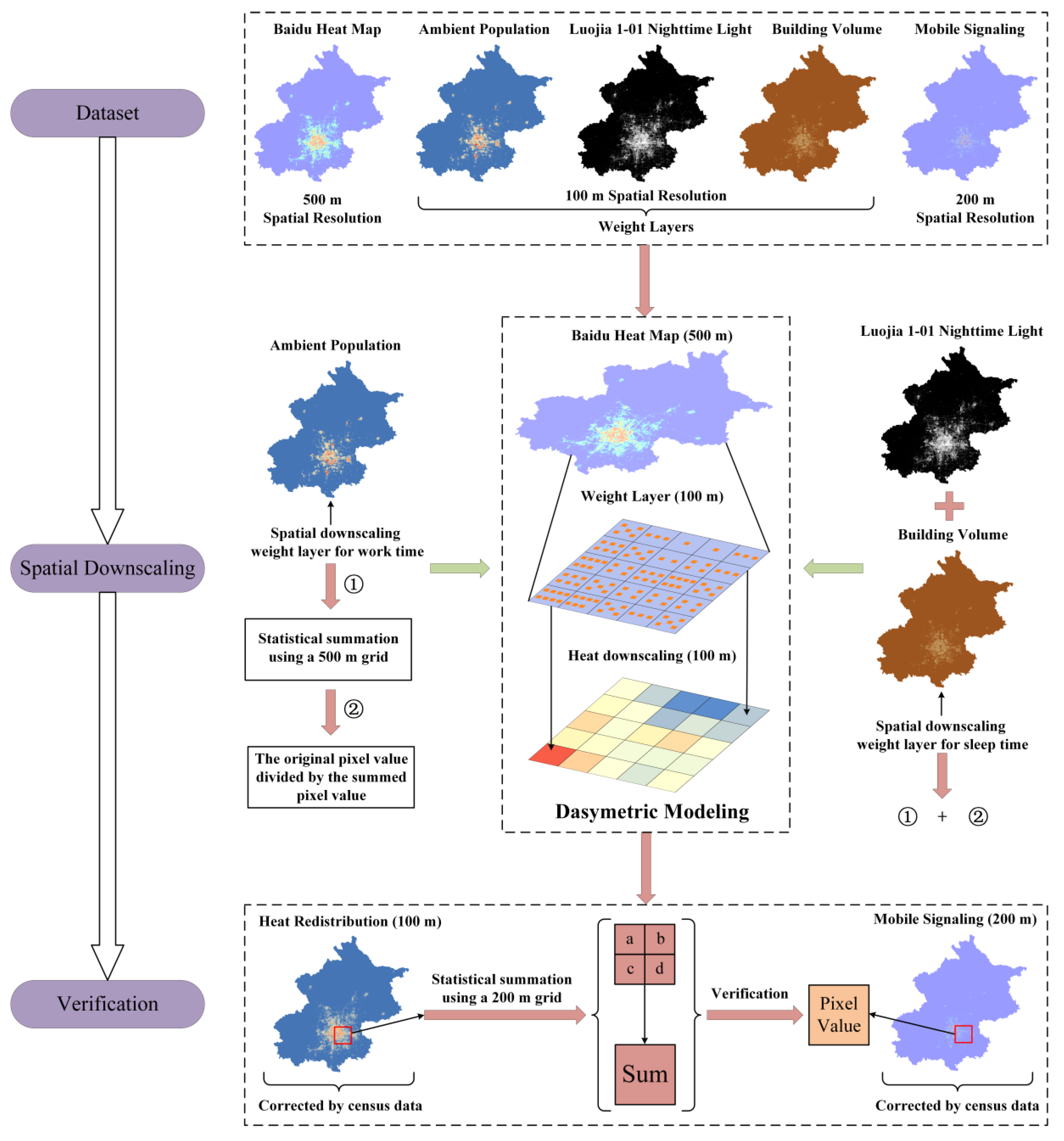
We proposed a spatial downscaling framework for Baidu heat map data to map the dynamic population distribution (see Figure 3). This spatial downscaling framework is divided into three parts: first, we preprocessed the relevant dataset; second, we generated the weight layers during work time and sleep time; and finally, we validated the results. In addition, we performed kernel density estimation on the reclassified POI data to reflect different land use types and used the random forest model to analyze the relationship between population density distribution and land use types in different time periods. The details are described in the following sections.

3.1. Spatial Downscaling Framework for Work Time

Since the sleep time and work time of different occupations are inconsistent, according to our understanding and references [1,48], we set the sleep time and work time of a regular weekday to 0:00–7:00 and 7:00–24:00, respectively. We employed an efficient dasymetric method to spatially downscale Baidu heat map data (500 m) to 100 m spatial resolution. Dasymetric mapping is an ancillary-driven method and has been widely used in spatial downscaling [25]. The dasymetric method introduces the density information from ancillary variables to redistribute the standardized data into a finer scale distribution. The critical step is the definition of weight layers, which is usually determined by the existing or assumed relationship between the standardized data and ancillary variables [60]. Each pixel value in ambient population data represents the relative magnitude of the probability of population presence during work time. Therefore, we used the ambient population data as a spatial downscaling weight layer for work time and assumed that the spatial distribution of Baidu heat map data (500 m) at finer scales (100 m) is the same as that of the ambient population data (100 m).
In this paper, we first created a fishnet with empty attributes at the 500 m × 500 m cell size covering all of Beijing in ArcGIS 10.6. Then, we used Equation (2) to count the sum of the 25 ambient population pixel values corresponding to each cell in the fishnet and used Equation (3) to count the weight of each pixel of ambient population data. Then, we used Equation (4) to spatially downscale each pixel of the Baidu heat map data. Since the Baidu heat map data are sampling data, the extracted heat values are not the actual population numbers but only the relative magnitude of population density [61]. We assumed that the total population of Beijing is constant during a day, and the daily inflow and outflow of the population are balanced. Therefore, we used the census data to correct the Baidu heat map data after spatial downscaling so that each pixel value represented the true population (see Equation (5) for the specific calculation process).
S i = j = 1 25 P j
W j = P j S i
H i j = H i × W j
H i j = H i j × C S
where P j is the pixel value of ambient population data, S i is the sum of the 25 ambient population pixel values corresponding to the i -th cell in the fishnet, W j is the weight value, H i is the i -th pixel value of Baidu heat map data, H i j is the pixel value of Baidu heat map data after spatial downscaling, S is the sum of all pixel values of Baidu heat map data after spatial downscaling, C is the total population of Beijing in 2020 (i.e., 21,893,095), and H i j is the true population value.

3.2. Spatial Downscaling Framework for Sleep Time

Our spatial downscaling framework during sleep time is almost the same as that during work time—the only difference is the definition of weight layer. We assumed that (1) the larger building volume can accommodate more people during sleep time and (2) in areas with missing building volume data, NTL intensity reflected the residence distribution across settlements (i.e., the brighter the NTL was, the larger the population would be during sleep time). Therefore, we integrated building volume and NTL as the weight layer of the spatial downscaling framework during sleep time.
Since building volume data are missing to varying degrees in urban and rural areas and NTL data can well reflect the population distribution of sleep time [28,35], we used NTL data to compensate for these missing data. However, the blooming effect is inherent to NTL and indicates that the NTL within a small land area inside a city can brighten surrounding areas [54]. Therefore, we chose to normalize the NTL data, kept the relative sizes between pixel values constant, and assigned their values to the corresponding pixels in the building volume data, which complemented the missing building volume information and did not affect the original building volume information by oversizing the pixel values. In this paper, we first normalized the Luojia 1-01 NTL data using Equation (6). Then, we used Equation (7) to add the corresponding pixel values from the building volume data and Luojia 1-01 NTL data to obtain a new raster layer. Finally, we used the new raster layer as the weight layer and followed the spatial downscaling process of work time to spatially downscale the Baidu heat map data during sleep time.
R L i = R L i R L m i n R L m a x     R L m i n
N i = { B V i + N T L i ,           B V i = 0                   B V i ,                             B V i > 0    
where R L i is the normalized value of the i -th pixel of the raster layer, R L i denotes the original value of the i -th pixel of the raster layer, R L m a x represents the maximum value of the raster layer, R L m i n is the minimum value of the raster layer, B V i is the i -th pixel value of building volume data, N T L i is the i -th pixel value of Luojia 1-01 NTL data, and N i is the i -th pixel value of the new raster layer.

3.3. Kernel Density Estimation and Random Forest

POI refers to all geographic entities that can be abstracted as points containing precise spatial information. POI categories are similar to land use categories, and the preferences and social functions of people can be well represented with POI; thus, all types of POI density can directly or indirectly reflect land use types and functional zoning [62]. Therefore, we used kernel density estimation (KDE) to calculate the density of POI for each functional type on a 100 m grid to reflect the percentage of different land use types. KDE is a method of reconstructing the probability of the spatial distribution of points and lines in accordance with the current locations of parts of points and lines [63]. In consideration of the spatial proximity of geographic units, KDE is often used to deal with datasets with spatial uncertainty and has been proven effective in yielding spatially smooth and near-reality results. The KDE method can be described as follows:
f ( x , y ) = i = 1 n k d 2 [ ( 1 ( x x i ) 2 + ( y y i ) 2 d 2 ) ] 2
where f ( x ) denotes the point density of the grid in location ( x , y ) , n denotes the number of observations, i denotes each observation, d denotes the bandwidth to define the size of smoothing, and k denotes a bivariate probability density function called the core. After the kernel function has been defined, the sliding window method was used to determine the point density of each grid [56].
Random forest (RF) is a tree-based machine learning model. It randomly extracts m sub-samples and k sub-features from the original dataset, forming multiple sets of sub-data for training multiple regression trees. Then, it applies the averaging method to combine the regression results of each regression tree and generate the final regression results. The random forest model introduces a random attribute selection process while training, which makes the diversity of the base regression trees come not only from the sample disturbance but also from the attribute disturbance. Therefore, the generalization performance of random forest can be further improved by increasing the difference degree between the base regression trees [64]. Due to the satisfactory performance of the random forest model, we used it to fit the complex nonlinear relationship between population distribution and land use type at different time periods.

3.4. Statistical Analysis and Accuracy Assessment

The statistical analysis metric used in this paper is the coefficient of variation (CV), which is a standardized measure of dispersion of a probability distribution or frequency distribution and is often used to compare the dispersion of datasets of different magnitudes [65]. Accuracy assessment is an important step to verify the accuracy of our spatial downscaling framework and the fitting precision of the random forest model, and it is the evaluation criterion for judging the results. Three widely used accuracy assessment metrics [24], namely the determination coefficient (R2), mean absolute error (MAE), and root mean square error (RMSE), were adopted in this study. The equations used to calculate the above four metrics are as follows:
C V = σ μ × 100 %
R 2 = i = 1 n ( y ^ i y ¯ ) 2 i = 1 n ( y i y ¯ ) 2
M A E = 1 n i = 1 n | y i y ^ i |
R M S E = 1 n i = 1 n ( y i y ^ i ) 2
where σ is the standard deviation of the dataset, μ is the average of the dataset, y i denotes the true value, y ^ i denotes the predicted value, y ¯ denotes the average of true values, and n denotes the total number of samples.

4. Results

4.1. Mapping Dynamic Population Distribution

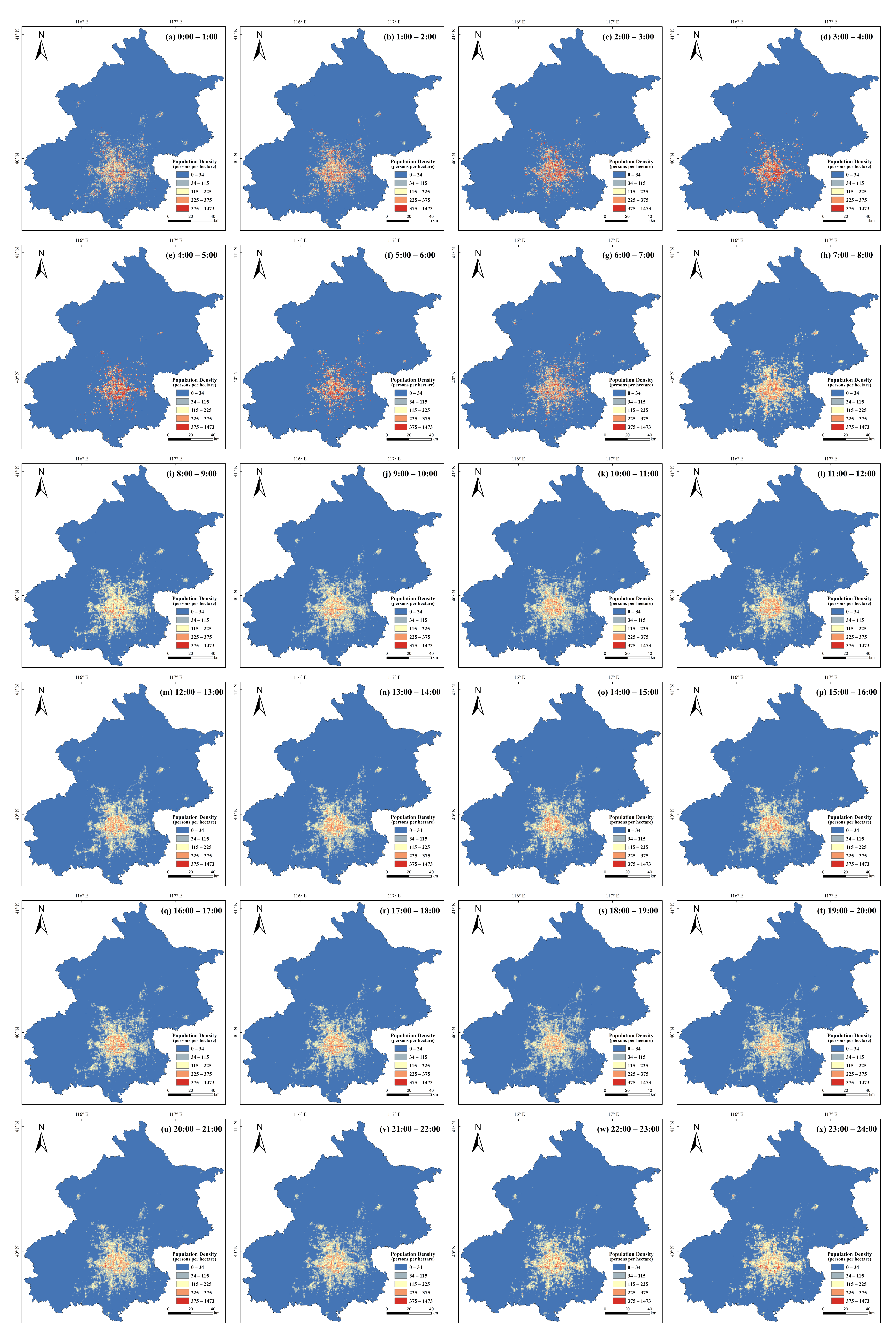
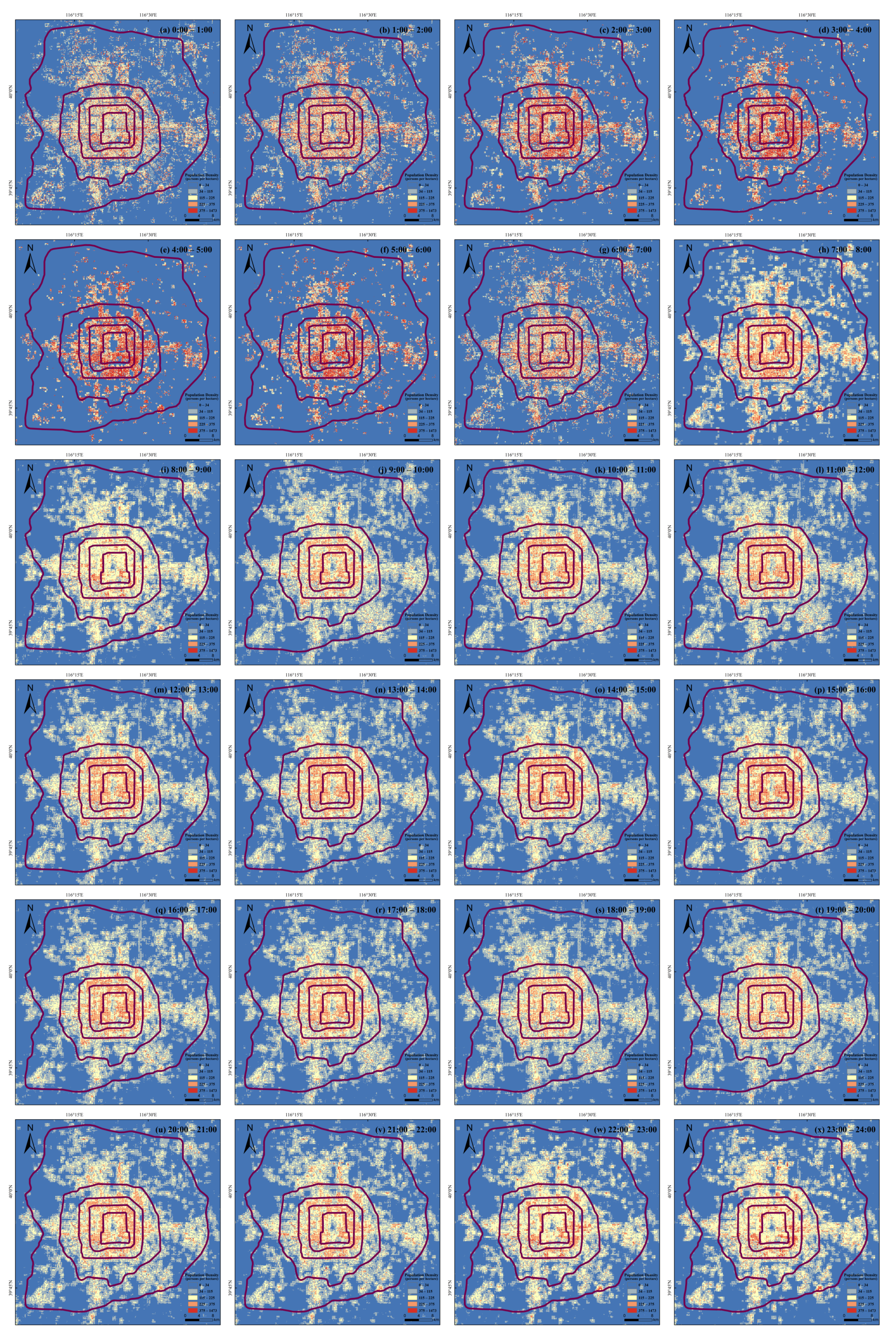
Based on the preprocessed correlation dataset and our proposed spatial downscaling framework during work time and sleep time, we spatially downscaled the Baidu heat map data for a total of 24 time periods in Beijing on 17 August 2022, and mapped the population density distribution with high spatiotemporal resolution (i.e., hourly, 100 m). The spatiotemporal patterns of the population show significant fluctuations between sleep time and work time, as shown in Figure 4 and Figure 5. During sleep time (i.e., 0:00–7:00), the population exhibits a high concentration, resulting in many areas with high population density and weak changes in the spatial distribution of population density during this period, which indicates a low intensity of population mobility. During work time (i.e., 7:00–24:00), it can be seen that the population is relatively dispersed, with a significant decrease in the number of areas with high population density, and the spatial distribution of population density changes significantly over time (e.g., significant changes in traffic flow), which indicates strong population mobility during this period. Overall, the high spatial and temporal resolution population distribution maps generated based on our proposed spatial downscaling framework can adequately capture the spatial heterogeneity of the population and the difference between sleep time and work time.

4.2. Evaluation of Spatial Downscaling Framework

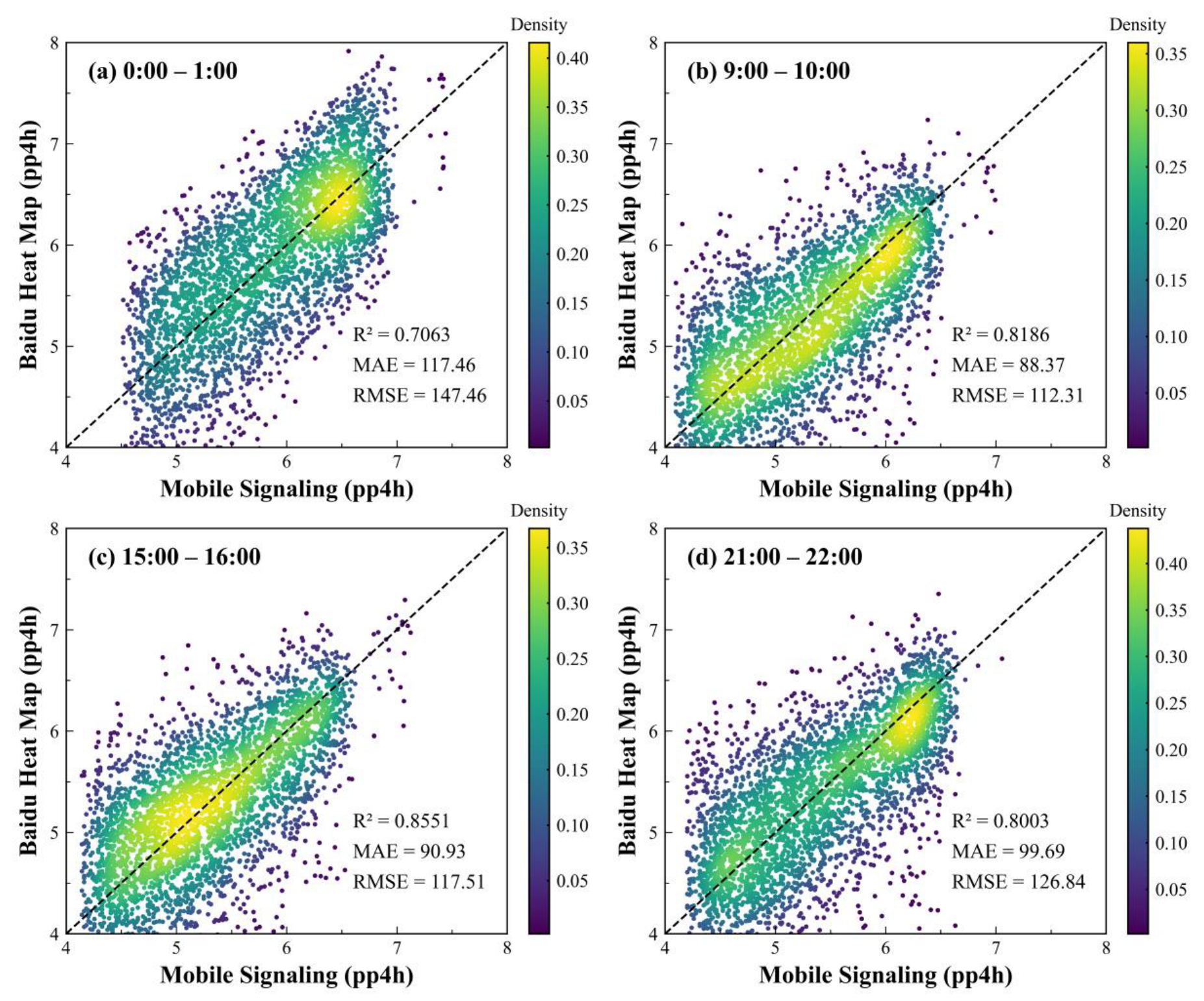
A rigorous accuracy evaluation process on the generated population distribution maps with high spatiotemporal resolution can illustrate the reliability of our proposed spatial downscaling framework. First, a fishnet with empty attributes at the 200 m × 200 m cell size covering all of Beijing was created in ArcGIS 10.6. Then, we used a 200 m fishnet to perform regional summation statistics on the population distribution maps for four time periods (i.e., 0:00–1:00, 9:00–10:00, 15:00–16:00, and 21:00–22:00), compared them with the 5172 mobile signaling data corrected by census data, and finally obtained the accuracy verification result (see Figure 3).
Figure 6 shows the accuracy evaluation results of the Baidu heat map population density for the four time periods, corresponding to one population distribution map generated by the spatial downscaling framework of sleep time and three population distribution maps generated by the spatial downscaling framework of work time. From the results, it should be noted that the precision (R2 = 0.7063, MAE = 117.46 persons/4 ha, RMSE = 147.46 persons/4 ha) of the population distribution map for the 0:00–1:00 time period is relatively lower than that of the other three time periods. We believe this phenomenon occurs because during sleep time, the frequency of different people using Baidu products decreases to different degrees, expanding the sampling bias of the data and leading to a change in the relative magnitude of the Baidu heat value [58,61], while the sampling bias of mobile signaling data as the true value fluctuates very little over time [45,50,66], thus making the accuracy assessment results for the 0:00–1:00 time period relatively lower. Overall, the scatters in all four time periods are distributed around the 1:1 line, which indicates that our population distribution maps in all four time periods have high accuracy and reflects the fact that our proposed spatial downscaling framework for the Baidu heat map during sleep time and work time can adequately characterize the accurate spatial changes in the population over time at finer scales.

5. Discussion

5.1. Spatiotemporal Distribution Characteristics of Population

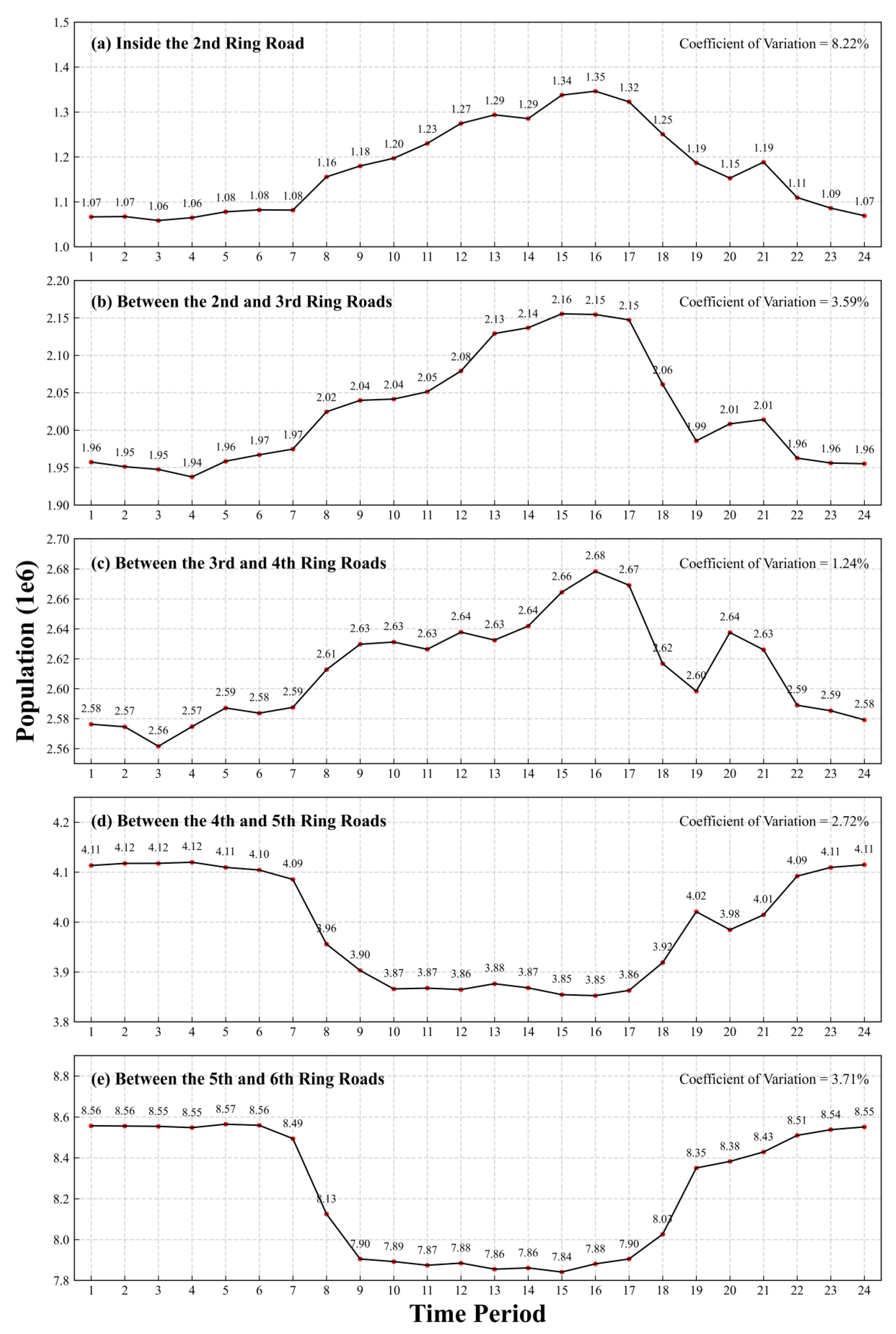
Since most people in Beijing live within the Sixth Ring Road, we used the generated dynamic population distribution maps to explore the evolution of the population spatial distribution within the Sixth Ring Road in Beijing over time on a regular weekday. Figure 7 illustrates the trend of the population between each ring road in Beijing over time. The population of different ring roads has a significant difference with time. From the perspective of the coefficient of variation, the population within the Second Ring Road has the most drastic change, and the population between the Third and Fourth Ring Roads has the flattest change. From the process of change, the populations within the Second Ring Road, between the Second and Third Ring Roads, and between the Third and Fourth Ring Roads present the trend of “stability–growth–decrease”, and the populations between the Fourth and Fifth Ring Roads and between the Fifth and Sixth Ring Roads present the trend of “stability–decrease–growth”.
Specifically, in each ring road, the population fluctuates smoothly during sleep time (i.e., 0:00–7:00) and dramatically during work time (i.e., 7:00–24:00), which is consistent with our understanding of the human activity patterns during sleep time and work time. In addition, a large number of the population changes were observed simultaneously among the five ring roads during the commuting time periods, 7:00–9:00 and 17:00–19:00. In China, with the establishment of the system of paid use of state-owned land, service spaces of commerce, finance, and business offices with strong ability to compete for rent are “embedded” in the core of cities, while industrial parks and residential areas with single functions are formed in the periphery, resulting in the separation of residential, working, and leisure spaces [48]. For Beijing, a large number of companies and firms are located within the Fourth Ring Road, and the high housing prices within the Fourth Ring Road lead to a large number of working people renting and buying houses between the Fourth and Sixth Ring Roads; thus, a substantial change in population numbers can be seen in these two commuting time periods [1,67]. Overall, the distribution of the population in Beijing on a regular weekday showed a “daytime centripetal, nocturnal centrifugation” difference in characteristics of time and space.

5.2. Relationship between Population and Land Use Type over Time

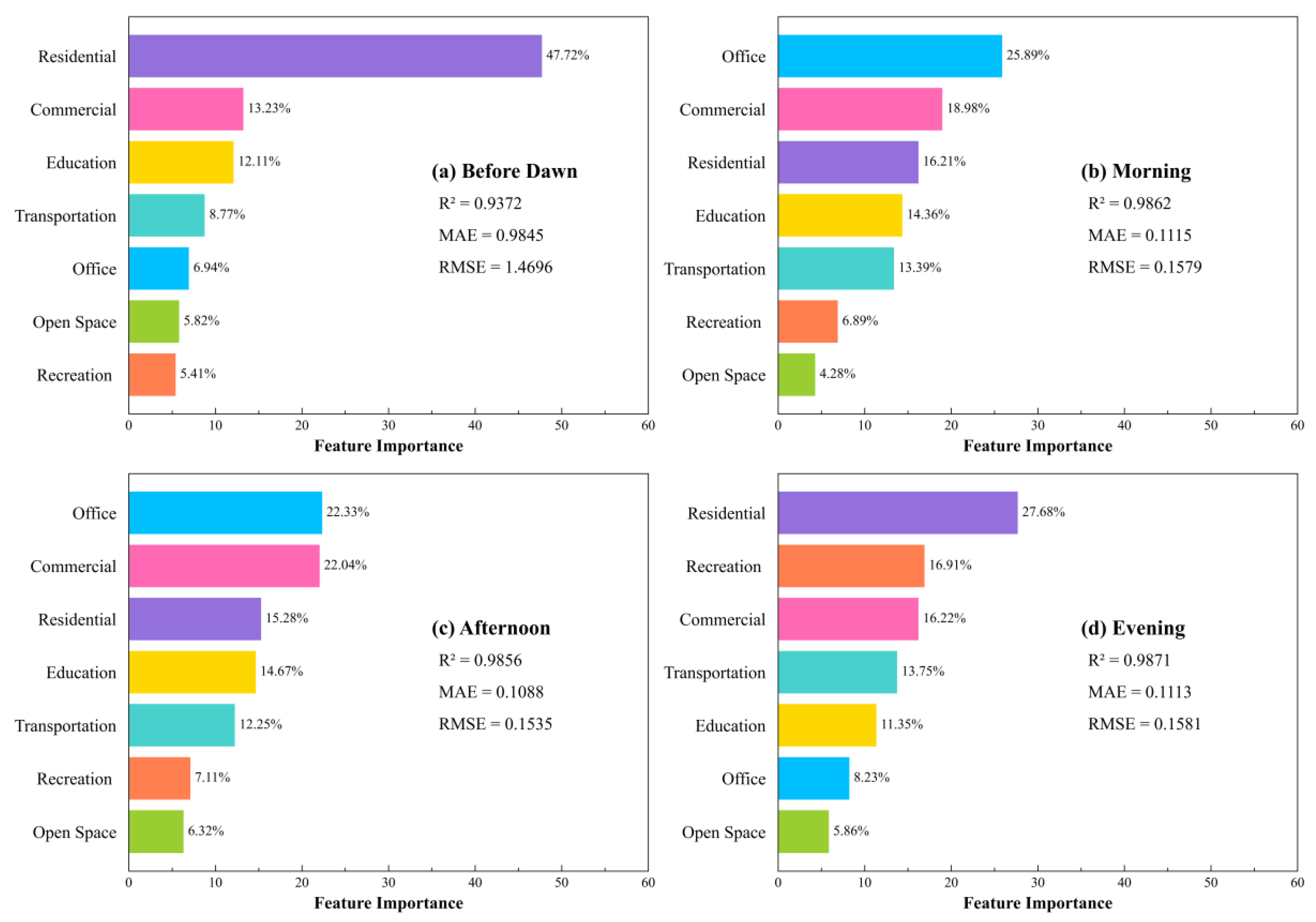
We used the KDE method to calculate the density of POI for seven functional types on a 100 m grid to reflect the percentage of different land use types. For convenience of processing, the population density distribution maps from 0:00 to 24:00 were divided into four time periods, i.e., 0:00–7:00 (before dawn), 7:00–13:00 (morning), 13:00–18:00 (afternoon), and 18:00–24:00 (evening), and we averaged the population density distribution maps for the four time periods. Then, we input the POI density of the seven functional types as the independent variable and the average population density as the dependent variable into the random forest model for fitting. After developing the RF model, each predictor variable had an output value (i.e., feature importance), indicating the contribution of the predictor variable to the target variable [34,64]. Finally, we used the feature importance to analyze the relationship between population density distribution and land use types at different time periods of a regular weekday. Figure 8 shows the results of the fitting accuracy and feature importance assessment.
The results of random forest regression show that all four time periods have high fitting accuracy, which indicates that the feature importance assessment has very high confidence [23]. From the perspective of the influencing factors and intensity, during the 0:00–7:00 time period, the population density distribution is mainly influenced by residential land use. During the 7:00–13:00 and 13:00–18:00 time periods, office land use and commercial land use dominate the population density distribution. During the 18:00–24:00 time period, residential land use, recreational land use, and commercial land use mainly affect the population density distribution. This indicates that residents′ activities on the regular weekday mainly consist of rest, work and recreational activities, which generally undergo the process of “rest activities–employment activities–leisure activities–rest activities”, which also is consistent with our expectations. On the other hand, the variation in the influencing factors and intensity reflects not only the daily activity patterns of residents but also the heterogeneity of urban functional zoning [48,49]. The spatiotemporal distribution of the population is actually a process in which residents choose the activity space in order to meet their own needs. Therefore, the interaction between the purpose of residents’ activities and the spatial functional differences leads to the spatiotemporal evolution of the population distribution.

5.3. Impact of Policy on Population Mobility during the COVID-19 Pandemic

Since the outbreak of COVID-19, China has made remarkable achievements in the fight against the epidemic. China has always adhered to the “surgical control and dynamic zero COVID-19” epidemic prevention and control policy, so it has maintained low infection and death rates [6,68]. Surgical control refers to the lockdown of only small-scale areas where there is a risk of outbreaks, and dynamic zero COVID-19 means finding an epidemic, eliminating the epidemic, and quickly cutting off the chain of transmission. The purpose of the policy is to keep people’s activities unrestricted and maintain people’s normal life to the greatest extent possible under the premise of ensuring people’s health. China’s policy for people in high-risk areas is not to leave their homes, those in medium-risk areas are not to leave their residential compounds, and those in low-risk areas are free to move around. On 17 August 2022, three cases of COVID-19 were reported in Beijing, and the government took control measures as quickly as possible, in which three high-risk buildings were delineated, and the remaining buildings in their corresponding residential compounds were classified as medium risk. We selected these three high-risk buildings, as well as three low-risk buildings in the residential compounds closest to the respective residential compounds of the three high-risk buildings for comparison. Table 3 shows the detailed information of these residential compounds and buildings. Finally, we used population distribution maps with high spatiotemporal resolution generated by our proposed spatial downscaling framework to analyze the execution of China’s COVID-19 epidemic prevention and control policy.
We summarized the raster values of the 100 m grid to which the buildings belonged and drew line graphs. Figure 9 shows the population mobility over time of the three high-risk buildings and three low-risk buildings. From the perspective of coefficient of variation, the population mobility intensity of the three high-risk buildings is very low, while the population mobility intensity of the corresponding three low-risk buildings is relatively high. This indicates that the high-risk buildings are in a lockdown state, strictly limiting the movement of the population, while the low-risk buildings are in an open state that the population can access freely. It is worth noting that the population of high-risk buildings fluctuates significantly during certain time periods. We believe that this phenomenon may be due to medical staff coming to perform nucleic acid testing, people from low- and medium-risk buildings in the same residential compound entering the vicinity of high-risk buildings, or because of the sampling bias of Baidu’s heat map data [7,8,48,58,61]. Overall, our results demonstrate the strong execution of China’s “surgical control and dynamic zero COVID-19” epidemic prevention and control policy. It was the superiority of that policy that safeguarded the lives and health of the Chinese people and liberated their freedom to the greatest extent possible.

5.4. Advantages and Limitations

Considering the importance and difficulty of mapping population distribution with high spatiotemporal resolution over large areas, we integrated ambient population data, nighttime light data, and building volume data and innovatively proposed a spatial downscaling framework for Baidu heat map data during work time and sleep time. After rigorous validation using mobile signaling data, the results show that our proposed spatial downscaling framework has excellent accuracy, and the generated population distribution maps with high spatiotemporal resolution can explore subtle changes in population density within cities over time. What we essentially propose is a spatial downscaling idea; regardless of what kind of data based on location services are used (e.g., Baidu heat map data, Tencent location big data, etc.) and regardless of the spatial resolution of the acquired data (e.g., 500 m, 400 m, etc.), this idea can be used to perform spatial downscaling on these dynamic data. In addition, the relevant data used in this paper are easily available, so our proposed spatial downscaling framework can be transferred to other regions, and once those data are obtained, the population density distribution can be mapped at a specific time period in a specific region.
Although our proposed spatial downscaling framework can effectively map the dynamic population distribution, it still has some limitations. The Baidu heat map data are sampled data, so there are some potential uncertainties, such as children and elderly people who do not have smartphones and those who have smartphones who do not install Baidu-related products, which can lead to some bias in the results [58,61]. Since work time and sleep time are different for people in different occupations, it is difficult to fully define the difference between these two time periods, so our division of these two time periods cannot cover everyone [1]. In addition, on weekends or other holidays, residents have more free time, the types of activities are more abundant, and the activities are more random [48]. Therefore, our ambient population data cannot be used as a spatial downscaling weight layer for these days, leading to limitations in the use of our spatial downscaling framework on these days. Although the nighttime light data we used from Luojia 1-01 have the highest spatial resolution of all nighttime light data available, Luojia 1-01 has stopped updating the data at present due to satellite itself design, resulting in inconsistent time matching between the acquired Luojia 1-01 NTL data and the Baidu heat map data, which may lead to incorrect pixel value assignment in the spatial downscaling process [55,56]. In summary, despite these objective limitations, this study still provides a method that can map the population distribution with high spatiotemporal resolution over a large area when a better solution is difficult to obtain.

6. Conclusions

In this study, we integrated ambient population data, nighttime light data, and building volume data; innovatively proposed a spatial downscaling framework for Baidu heat map data during work time and sleep time; and mapped the population distribution with high spatiotemporal resolution (i.e., hourly, 100 m) in Beijing. Then, we validated the generated population distribution maps with high spatiotemporal resolution using the highest-quality validation data (i.e., mobile signaling data). Finally, we performed correlation analysis. The major findings of this study are as follows:
(1)
Verification results show that our proposed spatial downscaling framework for both work time and sleep time has high accuracy.
(2)
The relevant statistical analysis indicates that the distribution of the population in Beijing on a regular weekday shows “centripetal centralization at daytime, centrifugal dispersion at night” spatiotemporal variation characteristics.
(3)
The results of the feature importance assessment indicate that the interaction between the purpose of residents’ activities and the spatial functional differences leads to the spatiotemporal evolution of the population distribution.
(4)
During the COVID-19 pandemic, China’s “surgical control and dynamic zero COVID-19” policy was strongly implemented, which ensured the life and freedom of movement of the Chinese people to the greatest extent possible.
In addition, our proposed spatial downscaling framework can be easily transferred to other regions due to the easy availability of relevant datasets, which is of great significance to explore the underlying mechanisms between environmental-related human diseases and various environmental problems. Future research can focus on refining complex human activity patterns and combining them with our proposed spatial downscaling framework to further improve accuracy.

Author Contributions

W.B.: Conceptualization, Methodology, Data curation, Validation, Visualization, Formal analysis, Writing—original draft. A.G.: Conceptualization, Methodology, Supervision, Writing—review and editing, Funding acquisition, Project administration. T.Z.: Data curation, Visualization. Y.Z.: Data curation, Validation. B.L.: Data curation, Validation. S.C.: Validation. All authors have read and agreed to the published version of the manuscript.

Funding

This research was jointly funded by the National Key Research and Development Program of China (grant number 2019YFE01277002) and the National Natural Science Foundation of China (grant number 41671412).

Institutional Review Board Statement

Not applicable.

Informed Consent Statement

Not applicable.

Data Availability Statement

Not applicable.

Acknowledgments

Many thanks to the anonymous reviewers and editors for providing valuable opinions for revising the manuscript.

Conflicts of Interest

The authors declare no conflict of interest.

References

  1. Zhao, X.; Zhou, Y.; Chen, W.; Li, X.; Li, X.; Li, D. Mapping hourly population dynamics using remotely sensed and geospatial data: A case study in Beijing, China. Gisci. Remote Sens. 2021, 58, 717–732. [Google Scholar] [CrossRef]
  2. Kuang, W.; Hou, Y.; Dou, Y.; Lu, D.; Yang, S. Mapping Global Urban Impervious Surface and Green Space Fractions Using Google Earth Engine. Remote. Sens. 2021, 13, 4187. [Google Scholar] [CrossRef]
  3. Kuang, W.; Zhang, S.; Li, X.; Lu, D. A 30 m resolution dataset of China’s urban impervious surface area and green space, 2000–Earth Syst. Sci. Data. 2021, 13, 63–82. [Google Scholar]
  4. Li, K.; Chen, Y.; Li, Y. The Random Forest-Based Method of Fine-Resolution Population Spatialization by Using the Inter-national Space Station Nighttime Photography and Social Sensing Data. Remote Sens. 2018, 10, 1650. [Google Scholar] [CrossRef] [Green Version]
  5. Li, B.; Gong, A.; Zeng, T.; Bao, W.; Xu, C.; Huang, Z. A Zoning Earthquake Casualty Prediction Model Based on Machine Learning. Remote. Sens. 2021, 14, 30. [Google Scholar] [CrossRef]
  6. Jia, J.S.; Lu, X.; Yuan, Y.; Xu, G.; Jia, J.; Christakis, N.A. Population flow drives spatio-temporal distribution of COVID-19 in China. Nature 2020, 582, 389–394. [Google Scholar] [CrossRef]
  7. Daughton, C.G. Wastewater surveillance for population-wide COVID-19: The present and future. Sci. Total. Environ. 2020, 736, 139631. [Google Scholar] [CrossRef]
  8. Han, Y.; Yang, L.; Jia, K.; Li, J.; Feng, S.; Chen, W.; Zhao, W.; Pereira, P. Spatial distribution characteristics of the COVID-19 pandemic in Beijing and its relationship with environmental factors. Sci. Total. Environ. 2020, 761, 144257. [Google Scholar] [CrossRef]
  9. Zhao, G.; Yang, M. Urban Population Distribution Mapping with Multisource Geospatial Data Based on Zonal Strategy. ISPRS Int. J. Geo-Inf. 2020, 9, 654. [Google Scholar] [CrossRef]
  10. Li, X.; Zhou, W. Dasymetric mapping of urban population in China based on radiance corrected DMSP-OLS nighttime light and land cover data. Sci. Total. Environ. 2018, 643, 1248–1256. [Google Scholar] [CrossRef]
  11. Pérez-Morales, A.; Gil-Guirado, S.; Martínez-García, V. Dasymetry Dash Flood (DDF). A Method Popul. Mapp. Flood Expo. Assess. Tour. Cities. Appl. Geography 2022, 142, 102683. [Google Scholar] [CrossRef]
  12. Tenerelli, P.; Gallego, J.F.; Ehrlich, D. Population density modelling in support of disaster risk assessment. Int. J. Disaster Risk Reduct. 2015, 13, 334–341. [Google Scholar] [CrossRef]
  13. Weber, E.M.; Seaman, V.Y.; Stewart, R.N.; Bird, T.J.; Tatem, A.J.; McKee, J.J.; Bhaduri, B.L.; Moehl, J.J.; Reith, A.E. Cen-sus-independent population mapping in northern Nigeria. Remote Sens. Environ. 2018, 204, 786–798. [Google Scholar]
  14. Li, L.; Li, J.; Jiang, Z.; Zhao, L.; Zhao, P. Methods of Population Spatialization Based on the Classification Information of Buildings from China’s First National Geoinformation Survey in Urban Area: A Case Study of Wuchang District, Wuhan City, China. Sensors 2018, 18, 2558. [Google Scholar] [CrossRef] [PubMed] [Green Version]
  15. Xie, Z. A Framework for Interpolating the Population Surface at the Residential-Housing-Unit Level. GIScience Remote Sens. 2006, 43, 233–251. [Google Scholar] [CrossRef]
  16. Langford, M. Obtaining population estimates in non-census reporting zones: An evaluation of the 3-class dasymetric method. Comput. Environ. Urban Syst. 2006, 30, 161–180. [Google Scholar] [CrossRef]
  17. Goodchild, M.F.; Lam, N. Interpolation—A Variant of the Traditional Spatial Problem. Geo-Processing 1980, 1, 297–312. [Google Scholar]
  18. Goodchild, M.F.; Anselin, L.; Deichmann, U. A Framework for the Areal Interpolation of Socioeconomic Data. Environ. Plan. A Econ. Space 1993, 25, 383–397. [Google Scholar] [CrossRef]
  19. Wang, L.; Wang, S.; Zhou, Y.; Liu, W.; Hou, Y.; Zhu, J.; Wang, F. Mapping population density in China between 1990 and 2010 using remote sensing. Remote Sens. Environ. 2018, 210, 269–281. [Google Scholar] [CrossRef]
  20. Lwin, K.K.; Sugiura, K.; Zettsu, K. Space–time multiple regression model for grid-based population estimation in urban areas. Int. J. Geogr. Inf. Sci. 2016, 30, 1579–1593. [Google Scholar] [CrossRef]
  21. Xu, Y.; Song, Y.; Cai, J.; Zhu, H. Population mapping in China with Tencent social user and remote sensing data. Appl. Geography 2021, 130, 102450. [Google Scholar] [CrossRef]
  22. Zhao, S.; Liu, Y.; Zhang, R.; Fu, B. China’s population spatialization based on three machine learning models. J. Clean. Prod. 2020, 256, 120644. [Google Scholar] [CrossRef]
  23. Qiu, G.; Bao, Y.; Yang, X.; Wang, C.; Ye, T.; Stein, A.; Jia, P. Local Population Mapping Using a Random Forest Model Based on Remote and Social Sensing Data: A Case Study in Zhengzhou, China. Remote Sens. 2020, 12, 1618. [Google Scholar] [CrossRef]
  24. Bao, W.; Gong, A.; Zhao, Y.; Chen, S.; Ba, W.; He, Y. High-Precision Population Spatialization in Metropolises Based on Ensemble Learning: A Case Study of Beijing, China. Remote Sens. 2022, 14, 3654. [Google Scholar] [CrossRef]
  25. Jia, P.; Gaughan, A.E. Dasymetric modeling: A hybrid approach using land cover and tax parcel data for mapping population in Alachua County, Florida. Appl. Geography 2016, 66, 100–108. [Google Scholar] [CrossRef]
  26. Gaughan, A.E.; Stevens, F.R.; Huang, Z.; Nieves, J.J.; Sorichetta, A.; Lai, S.; Ye, X.; Linard, C.; Hornby, G.M.; Hay, S.I.; et al. Spatiotemporal patterns of population in mainland China, 1990 to 2010. Sci. Data 2016, 3, 160005. [Google Scholar] [CrossRef] [Green Version]
  27. Zhou, Y.; Ma, M.; Shi, K.; Peng, Z. Estimating and Interpreting Fine-Scale Gridded Population Using Random Forest Re-gression and Multisource Data. ISPRS Int. J. Geo-Information. 2020, 9, 369. [Google Scholar] [CrossRef]
  28. Elvidge, C.D.; Baugh, K.E.; Dietz, J.B.; Bland, T.; Sutton, P.C.; Kroehl, H.W. Radiance Calibration of DMSP-OLS Low-Light Imaging Data of Human Settlements. Remote Sens. Environ. 1999, 68, 77–88. [Google Scholar] [CrossRef]
  29. Briggs, D.J.; Gulliver, J.; Fecht, D.; Vienneau, D.M. Dasymetric modelling of small-area population distribution using land cover and light emissions data. Remote Sens. Environ. 2007, 108, 451–466. [Google Scholar] [CrossRef]
  30. Lu, D.; Tian, H.; Zhou, G.; Ge, H. Regional mapping of human settlements in southeastern China with multisensor remotely sensed data. Remote Sens. Environ. 2008, 112, 3668–3679. [Google Scholar] [CrossRef]
  31. Kuang, W. 70 years of urban expansion across China: Trajectory, pattern, and national policies. Sci. Bull. 2020, 65, 1970–1974. [Google Scholar] [CrossRef]
  32. Kuang, W.; Du, G.; Lu, D.; Dou, Y.; Li, X.; Zhang, S.; Chi, W.; Dong, J.; Chen, G.; Yin, Z.; et al. Global observation of urban expansion and land-cover dynamics using satellite big-data. Sci. Bull. 2020, 66, 297–300. [Google Scholar] [CrossRef]
  33. Kuang, W.; Liu, J.; Tian, H.; Shi, H.; Dong, J.; Song, C.; Li, X.; Du, G.; Hou, Y.; Lu, D.; et al. Cropland redistribution to marginal lands undermines environmental sustainability. Natl. Sci. Rev. 2021, 9, nwab091. [Google Scholar] [CrossRef] [PubMed]
  34. Ye, T.; Zhao, N.; Yang, X.; Ouyang, Z.; Liu, X.; Chen, Q.; Hu, K.; Yue, W.; Qi, J.; Li, Z.; et al. Improved population mapping for China using remotely sensed and points-of-interest data within a random forests model. Sci. Total. Environ. 2018, 658, 936–946. [Google Scholar] [CrossRef] [PubMed]
  35. Wang, Y.; Huang, C.; Zhao, M.; Hou, J.; Zhang, Y.; Gu, J. Mapping the Population Density in Mainland China using NPP/VIIRS and Points-Of-Interest Data Based on a Random Forests Model. Remote Sens. 2020, 12, 3645. [Google Scholar] [CrossRef]
  36. Esch, T.; Brzoska, E.; Dech, S.; Leutner, B.; Palacios-Lopez, D.; Metz-Marconcini, A.; Marconcini, M.; Roth, A.; Zeidler, J. World Settlement Footprint 3D—A first three-dimensional survey of the global building stock. Remote Sens. Environ. 2022, 270, 112877. [Google Scholar] [CrossRef]
  37. Frantz, D.; Schug, F.; Okujeni, A.; Navacchi, C.; Wagner, W.; van der Linden, S.; Hostert, P. National-scale mapping of building height using Sentinel-1 and Sentinel-2 time series. Remote Sens. Environ. 2020, 252, 112128. [Google Scholar] [CrossRef]
  38. Cao, Y.; Huang, X. A deep learning method for building height estimation using high-resolution multi-view imagery over urban areas: A case study of 42 Chinese cities. Remote Sens. Environ. 2021, 264, 112590. [Google Scholar] [CrossRef]
  39. Dobson, J.E.; Bright, E.A.; Coleman, P.R.; Durfee, R.C.; Worley, B.A. LandScan: A global population database for estimating populations at risk. Photogramm. Eng. Remote Sens. 2000, 66, 849–857. [Google Scholar]
  40. Bhaduri, B.; Bright, E.; Coleman, P.; Urban, M.L. LandScan USA: A high-resolution geospatial and temporal modeling approach for population distribution and dynamics. Geojournal 2007, 69, 103–117. [Google Scholar] [CrossRef]
  41. Stevens, F.R.; Gaughan, A.E.; Linard, C.; Tatem, A.J. Disaggregating Census Data for Population Mapping Using Random Forests with Remotely-Sensed and Ancillary Data. PLoS ONE 2015, 10, e0107042. [Google Scholar] [CrossRef] [PubMed] [Green Version]
  42. Batista E Silva, F.; Freire, S.; Schiavina, M.; Rosina, K.; Marin-Herrera, M.A.; Ziemba, L.; Craglia, M.; Koomen, E.; Lavalle, C. Uncovering temporal changes in Europe’s population density patterns using a data fusion approach. Nat. Commun. 2020, 11. [Google Scholar] [CrossRef] [PubMed]
  43. Zheng, Z.; Zhang, G. The Prediction of Finely-Grained Spatiotemporal Relative Human Population Density Distributions in China. IEEE Access 2020, 8, 181534–181546. [Google Scholar] [CrossRef]
  44. Khodabandelou, G.; Gauthier, V.; Fiore, M.; El-Yacoubi, M.A. Estimation of Static and Dynamic Urban Populations with Mobile Network Metadata. IEEE Trans. Mob. Comput. 2018, 18, 2034–2047. [Google Scholar] [CrossRef]
  45. Deville, P.; Linard, C.; Martin, S.; Gilbert, M.; Stevens, F.R.; Gaughan, A.E.; Blondel, V.D.; Tatem, A.J. Dynamic population mapping using mobile phone data. Proc. Natl. Acad. Sci. USA 2014, 111, 15888–15893. [Google Scholar] [CrossRef] [Green Version]
  46. Gu, J.; Xu, P.; Pang, Z.; Chen, Y.; Ji, Y.; Chen, Z. Extracting typical occupancy data of different buildings from mobile posi-tioning data. Energ. Build. 2018, 180, 135–145. [Google Scholar]
  47. Panczak, R.; Charles-Edwards, E.; Corcoran, J. Estimating temporary populations: A systematic review of the empirical literature. Palgrave Commun. 2020, 6, 1–10. [Google Scholar] [CrossRef]
  48. Li, J.; Li, J.; Yuan, Y.; Li, G. Spatiotemporal distribution characteristics and mechanism analysis of urban population density: A case of Xi’an, Shaanxi, China. Cities 2019, 86, 62–70. [Google Scholar] [CrossRef]
  49. Zhang, W.; Chong, Z.; Li, X.; Nie, G. Spatial patterns and determinant factors of population flow networks in China: Analysis on Tencent Location Big Data. Cities 2020, 99, 102640. [Google Scholar] [CrossRef]
  50. Zhang, G.; Rui, X.; Poslad, S.; Song, X.; Fan, Y.; Wu, B. A Method for the Estimation of Finely-Grained Temporal Spatial Human Population Density Distributions Based on Cell Phone Call Detail Records. Remote Sens. 2020, 12, 2572. [Google Scholar] [CrossRef]
  51. Khan, W.Z.; Xiang, Y.; Aalsalem, M.Y.; Arshad, Q. Mobile Phone Sensing Systems: A Survey. IEEE Commun. Surv. Tutor. 2012, 15, 402–427. [Google Scholar] [CrossRef]
  52. Zhang, G.; Poslad, S.; Fan, Y.; Rui, X. Quantitative spatiotemporal impact of dynamic population density changes on the COVID-19 pandemic in China’s mainland. Geo-Spatial Inf. Sci. 2022, 1–22. [Google Scholar] [CrossRef]
  53. Small, C.; Pozzi, F.; Elvidge, C.D. Spatial analysis of global urban extent from DMSP-OLS night lights. Remote Sens. Environ. 2005, 96, 277–291. [Google Scholar] [CrossRef]
  54. Cao, X.; Hu, Y.; Zhu, X.; Shi, F.; Zhuo, L.; Chen, J. A simple self-adjusting model for correcting the blooming effects in DMSP-OLS nighttime light images. Remote Sens. Environ. 2019, 224, 401–411. [Google Scholar] [CrossRef]
  55. Wang, C.; Chen, Z.; Yang, C.; Li, Q.; Wu, Q.; Wu, J.; Zhang, G.; Yu, B. Analyzing parcel-level relationships between Luojia 1-01 nighttime light intensity and artificial surface features across Shanghai, China: A comparison with NPP-VIIRS data. Int. J. Appl. Earth Obs. Geoinform. 2020, 85, 101989. [Google Scholar] [CrossRef]
  56. Wang, L.; Fan, H.; Wang, Y. Improving population mapping using Luojia 1-01 nighttime light image and location-based social media data. Sci. Total Environ. 2020, 730, 139148. [Google Scholar] [CrossRef]
  57. Fan, Z.; Duan, J.; Lu, Y.; Zou, W.; Lan, W. A geographical detector study on factors influencing urban park use in Nanjing, China. Urban For. Urban Green. 2021, 59, 126996. [Google Scholar] [CrossRef]
  58. Zhang, S.; Zhang, W.; Wang, Y.; Zhao, X.; Song, P.; Tian, G.; Mayer, A. Comparing Human Activity Density and Green Space Supply Using the Baidu Heat Map in Zhengzhou, China. Sustainability 2020, 12, 7075. [Google Scholar] [CrossRef]
  59. Elvidge, C.; Zhizhin, M.; Ghosh, T.; Hsu, F.-C.; Taneja, J. Annual Time Series of Global VIIRS Nighttime Lights Derived from Monthly Averages: 2012 to 2019. Remote Sens. 2021, 13, 922. [Google Scholar] [CrossRef]
  60. Leyk, S.; Gaughan, A.E.; Adamo, S.B.; de Sherbinin, A.; Balk, D.; Freire, S.; Rose, A.; Stevens, F.R.; Blankespoor, B.; Frye, C.; et al. The spatial allocation of population: A review of large-scale gridded population data products and their fitness for use. Earth Syst. Sci. Data 2019, 11, 1385–1409. [Google Scholar] [CrossRef] [Green Version]
  61. Feng, D.; Tu, L.; Sun, Z. Research on Population Spatiotemporal Aggregation Characteristics of a Small City: A Case Study on Shehong County Based on Baidu Heat Maps. Sustainability 2019, 11, 6276. [Google Scholar] [CrossRef] [Green Version]
  62. Wu, C.; Ye, X.; Ren, F.; Du, Q. Check-in behaviour and spatio-temporal vibrancy: An exploratory analysis in Shenzhen, China. Cities 2018, 77, 104–116. [Google Scholar] [CrossRef]
  63. Anderson, T.K. Kernel density estimation and K-means clustering to profile road accident hotspots. Accid. Anal. Prev. 2009, 41, 359–364. [Google Scholar] [CrossRef] [PubMed]
  64. Breiman, L. Random forests. Mach. Learn. 2001, 45, 5–32. [Google Scholar] [CrossRef] [Green Version]
  65. Zhang, J.-H.; Chung, T.D.Y.; Oldenburg, K.R. A Simple Statistical Parameter for Use in Evaluation and Validation of High Throughput Screening Assays. SLAS Discov. Adv. Sci. Drug Discov. 1999, 4, 67–73. [Google Scholar] [CrossRef]
  66. Chin, K.; Huang, H.; Horn, C.; Kasanicky, I.; Weibel, R. Inferring fine-grained transport modes from mobile phone cellular signaling data. Comput. Environ. Urban Syst. 2019, 77, 101348. [Google Scholar] [CrossRef]
  67. Ma, Y.; Xu, W.; Zhao, X.; Li, Y. Modeling the Hourly Distribution of Population at a High Spatiotemporal Resolution Using Subway Smart Card Data: A Case Study in the Central Area of Beijing. ISPRS Int. J. Geo-Inf. 2017, 6, 128. [Google Scholar] [CrossRef] [Green Version]
  68. Zhu, S.; Feng, S.; Ning, X.; Zhou, Y. Analysis of China’s fight against COVID-19 from the perspective of policy tools-policy capacity. Front. Public Health 2022, 10, 951941. [Google Scholar] [CrossRef]
Figure 1. Geographical location and overall situation of Beijing.
Remotesensing 15 00458 g001
Figure 2. Vector point display of Baidu heat map data (a) and mobile signaling data (b).
Remotesensing 15 00458 g002
Figure 3. A spatial downscaling framework for Baidu heat map during work time and sleep time.
Remotesensing 15 00458 g003
Figure 4. Estimated dynamic population distribution in Beijing on 17 August 2022.
Remotesensing 15 00458 g004
Figure 5. Estimated dynamic population distribution within the Sixth Ring Road in Beijing.
Remotesensing 15 00458 g005
Figure 6. Scatterplots of the Baidu heat map population density and the mobile signaling population density (total of 5172 pixels). A ln-ln transformation was conducted for the population density. The black dashed line indicates the 1:1 line. pp4 h: persons per 4 hectares.
Remotesensing 15 00458 g006
Figure 7. Spatiotemporal variation in population between ring roads in Beijing during a regular weekday. The numbers in the horizontal coordinates represent each of the 24 time periods of the day (i.e., 0:00–1:00, 1:00–2:00, 2:00–3:00, 3:00–4:00, etc.).
Remotesensing 15 00458 g007
Figure 8. Results of random forest model fitting accuracy and feature importance assessment.
Remotesensing 15 00458 g008
Figure 9. Population mobility over time of the three high-risk buildings and three low-risk buildings (ac). The numbers in the horizontal coordinates represent each of the 24 time periods of the day (i.e., 0:00–1:00, 1:00–2:00, 2:00–3:00, 3:00–4:00, etc.).
Remotesensing 15 00458 g009
Table 1. List of datasets and sources used in the study.
CategoryDatasetsFormatTimeSources
Geospatial big dataBaidu heat mapVector (Point)17 August 2022Baidu Map Services, China
Point of interestVector (Point)2020AMap Services, China
Building volumeVector (Polygon)2020Baidu Map Services, China
Remote sensing dataLuojia 1-01
nighttime light image
Raster (130 m)6 September 2018Hubei Data and
Application Center, China
NPP-VIIRS
nighttime light image
Raster (500 m)September 2018Earth Observation Group, USA
Population dataCensus dataTable2020Beijing Government, China
Ambient populationRaster (100 m)2020Bao et al. [24]
Validation dataMobile signalingVector (Point)17 August 2022China Mobile Operator
China Unicom Operator
China Telecom Operator
Basic geographic dataRing roadsVector (Polyline)2020Map World, China
Boundary mapsVector (Polygon)2020Map World, China
Table 2. The list of reclassified functional categories of POI.
Functional CategoryBig CategoryMid Category
OfficeEnterprisesAll
Medical ServiceAll
Daily Life ServiceAll
Commercial HouseIndustrial Park and Building
Finance and Insurance ServiceAll except ATM
Science/Culture and Education ServiceAll except school
Governmental Organization and Social GroupAll
EducationScience/Culture and Education ServiceSchool
RecreationTourist AttractionAll
Sports and RecreationAll
ResidentialCommercial HouseResidential Area
Open SpacePlace Name and AddressNatural Place Name
CommercialShoppingAll
Auto RepairAll
Auto ServiceAll
Auto DealersAll
Motorcycle ServiceAll
Food and BeveragesAll
Accommodation ServiceAll
TransportationRoad FurnitureAll
Transportation ServiceAll except parking lot
Place Name and AddressTransportation Place Name
UnclassifiedPass FacilitiesAll
Public FacilityAll
Indoor facilitiesAll
Commercial HouseCommercial House Related
Incidents and EventsAll
Transportation ServiceParking Lot
Place Name and AddressAll except natural place name
and transportation place name
Finance and Insurance ServiceATM
Table 3. Details of the three low-risk buildings and three high-risk buildings.
Residential CompoundBuildingDistrictStatusLatitude (N)Longitude (E)
JintaichengliwanNumber 9FengtaiLow-risk (Open)39.868516116.335501
LixinjiayuannanquNumber 1FengtaiHigh-risk (Lockdown)39.871384116.336488
JinbaohuayuanbeiquNumber 8ShunyiLow-risk (Open)40.176438116.656291
lunengqihaoyuanxiyuanNumber 36ShunyiHigh-risk (Lockdown)40.182606116.659425
BolinzaixianNumber 2ChangpingLow-risk (Open)40.110905116.449914
RongshangweilaiNumber 1ChangpingHigh-risk (Lockdown)40.109944116.459685
Disclaimer/Publisher’s Note: The statements, opinions and data contained in all publications are solely those of the individual author(s) and contributor(s) and not of MDPI and/or the editor(s). MDPI and/or the editor(s) disclaim responsibility for any injury to people or property resulting from any ideas, methods, instructions or products referred to in the content.