Article

Observations of the Boundary Layer in the Cape Grim Coastal Region: Interaction with Wind and the Influences of Continental Sources

1
School of Ecology and Environment, Beijing Technology and Business University, Beijing 100048, China
2
School of Earth Sciences, University of Melbourne, Melbourne, VIC 3010, Australia
3
Climate Science Centre, Oceans and Atmosphere, Commonwealth Scientific and Industrial Research Organization, Aspendale, VIC 3195, Australia
4
Observing Systems and Operations, Bureau of Meteorology, Smithton, TAS 7330, Australia
5
Australian Nuclear Science and Technology Organization, Sydney, NSW 2234, Australia
6
School of Earth, Atmosphere and Life Sciences, University of Wollongong, Wollongong, NSW 2522, Australia
7
Institutes of Physical Science and Information Technology, Anhui University, Hefei 230031, China
*
Author to whom correspondence should be addressed.
Remote Sens. 2023, 15(2), 461; https://doi.org/10.3390/rs15020461
Submission received: 6 December 2022 / Revised: 10 January 2023 / Accepted: 11 January 2023 / Published: 12 January 2023
(This article belongs to the Section Atmospheric Remote Sensing)

Abstract

:
A comparative study and evaluation of boundary layer height (BLH) estimation was conducted during an experimental campaign conducted at the Cape Grim Air Pollution station, Australia, from 1 June to 13 July 2019. The temporal and spatial distributions of BLH were studied using data from a ceilometer, sodar, in situ meteorological measurements, and back-trajectory analyses. Generally, the BLH under continental sources is lower than that under marine sources. The BLH is featured with a shallow depth of 515 ± 340 m under the Melbourne/East Victoria continental source. Especially the mixed continental sources (Melbourne/East Victoria and Tasmania direction) lead to a rise in radon concentration and lower BLH. In comparison, the boundary layer reaches a higher averaged BLH value of 730 ± 305 m when marine air is prevalent. The BLH derived from ERA5 is positively biased compared to the ceilometer observations, except when the boundary layer is stable. The height at which wind profiles experience rapid changes corresponds to the BLH value. The wind flow within the boundary layer increased up to ∼200 m, where it then meandered up to ∼300 m. Furthermore, the statistic shows that BLH is positively associated with near-surface wind speed. This study firstly provides information on boundary layer structure in Cape Grim and the interaction with wind, which may aid in further evaluating their associated impacts on the climate and ecosystem.

1. Introduction

The boundary layer is the lowest portion of the troposphere and is directly influenced by and responds to the Earth’s surface forcings, i.e., frictional drag, evaporation and transpiration, and sensible heat transfer in a one-hour or shorter period [1]. The depth of this layer, also known as the boundary layer height (BLH), is one of the most important quantities that is estimated in many dispersions model, as it influences the volume of air accessible for pollutant dispersion and the consequent concentrations [2,3]. Especially over the ocean, the representation of marine BLH processes, together with the optical properties of marine particles, has been recognized as an essential ingredient of atmospheric and atmosphere–ocean coupled models [4,5]. Therefore, the continuous observation of the BLH near the coast, with high vertical and temporal resolution, is thus desirable to support weather and air-quality prediction.
The characteristics of BLH over the ocean are influenced by sea surface wind speed, sea state, atmospheric stability, and sea surface temperature. They also depend on the wave field, which in turn is determined by factors such as wind speed and distance to the coast (fetch). Among the above factors, the boundary layer flow is particularly affected by wind shears, which modify both its internal structure and integral behavior, to the extent that these effects cannot be generally ignored. However, the details of the boundary layer structure and the wind information near the coast rely heavily on data that is relatively sparse and especially rare. Especially few observational studies are available over the Southern Ocean. The Cape Grim campaign offered an opportunity to explore the interaction between the boundary layer structure and its interaction with meteorological information.
Active remote sensing of meteorological parameters, trace gases, and aerosols using lidar, ceilometers, sodars, and wind profilers are among the most effective technologies for continuous BLH measurements. Ground-based lidar has been widely utilized to evaluate BLH by detecting aerosol backscatter with high temporal and spatial resolutions [6,7,8,9,10,11,12]. Attenuated backscatter signals can be employed to infer boundary layer dynamics, such as BLH, and the existence of a residual layer. The main assumption used to derive BLH from backscatter profiles is that the boundary layer has a relatively consistent aerosol concentration that is considerably greater than that of the air above. Besides aerosols, radon can also be taken as a tracer to illustrate the stability state of the boundary layer [13,14,15] and estimate the BLH [16,17,18].
Multiple lidar techniques have been developed to determine the BLH, including the gradient detection algorithm [19,20,21], curve fitting [22], the wavelet covariance technique [23,24,25], and identifying maximum signal variance [26,27]. More recent studies have been focused on more sophisticated algorithms including advanced techniques. For example, de Bruine et al. [28] imposed continuity constraints (both vertically and in time) in BLH estimates using the graph theory (pathfinder algorithm). Machine learning takes advantage of a K-means unsupervised algorithm to estimate BLH, as shown in Rieutord et al. [29]. More image processing methods [30,31,32] have also been developed. These studies demonstrate that identifying BLH from aerosol lidar is still an open area of research. Our study determines the BLH daily evolution based on the image edge detection (IED) method. Compared to similar morphology-based technology, our IED method relies on a single Canny edge detection, without combing with wavelet technology [31] or further filtering based on mathematical morphology and an object-based analysis [32]. However, the seemingly straightforward IED with an automatic determined threshold could provide robust BLH under certain conditions. More details can be found in the processing steps in Section 3. Two lidar-type instruments (ceilometer and sodar) for BLH estimation at a coastal site are investigated. The BLH results are also compared with those from the European Centre for Medium-Range Weather Forecasts (ECMWF)-ERA5 reanalysis. Meteorological variables, including wind speed (WS), wind direction (WD), ambient temperature (T), and radon concentration from the Cape Grim observation site, are used to study the BLH variation under different sources.
This study aims to depict the spatial–temporal structure of BLH variability in winter Cape Grim, thereby complementing the spatial and/or temporal details of vertical BLH and wind information observational studies that are scarce in the Southern Ocean. Specifically, the main goals of the present study are to (1) examine the interaction between the boundary layer (ceilometer) and wind profiles (sodar) and (2) investigate the impact of different sources, particularly the continental source, on the boundary layer evolution in the coastal region. The paper is organized as follows. Section 2 presents the site and measurement data. Section 3 explains the procedure of the IED approach. Section 4 investigates the findings of the ceilometer-BLH for two event studies (3 June 2019 and 25 June 2019), with the sodar wind profiles as ancillary measurements. Section 5 provides a statistical analysis of the wind effect on the BLH, and Section 6 concludes with a brief conclusion.

2. Site, Measurements, and Model Data
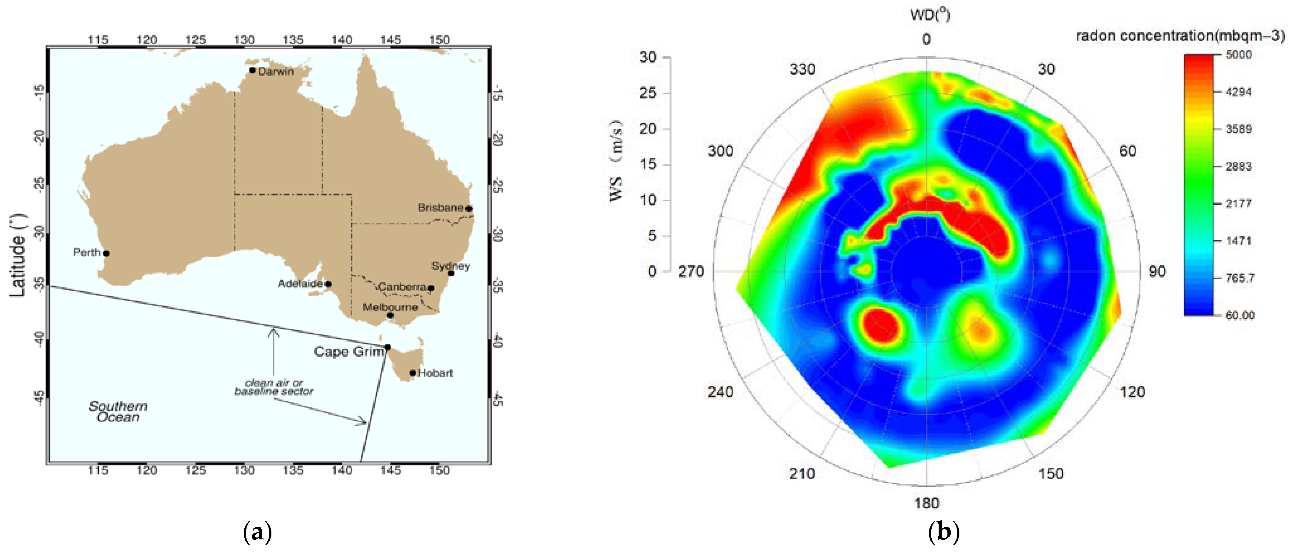
2.1. Site

The Cape Grim Baseline Air Pollution Station is located near the island state of Tasmania’s northwestern tip, Australia, at 40.7°S latitude and 144.7°E longitude (see Figure 1a). The station is perched atop a cliff 94 m above mean sea level. When the wind is blowing from the southwest sector, the air that reaches the station is classified as the clean and baseline air and typically has back tracking over the Southern Ocean of several days. Northwest Tasmania has a mild temperate climate, with average temperatures of 15 ± 2 °C, relative humidity of 75 ± 12%, wind speed of 9 ± 4 ms−1 (where ± is 1 standard deviation), and 25 mm of precipitation. Radon, which is ubiquitous in most rock and soil types, can be taken as the indicator of continental sources [33]. Figure 1b illustrates the potential sources of radon concentration during the observing period. The main contributors to radon are divided into three sources: (1) North/Northeast winds from Melbourne/Eastern Victoria source (WD: 0–60°); (2) Southwest winds from Baseline Sector (WD: 190–280°), probably due to the long-range transported soil or smoke; and (3) Northwest winds from Western Australia (WD: 300–360°). South/Southeast winds from Northern Tasmania (NT, 120–180°) contribute the least to the radon concentration in this study.

2.2. Measurements

2.2.1. Ceilometer

Ceilometers derive the BLH from vertical aerosol profiles, which are defined by Deadorff [34] as the height where there are equal areas of clear air above and particulates below. As a result, the BLH is regarded as the midpoint of the transition zone between the areas of elevated and diminished backscattering, i.e., the top of the aerosol layer [19]. The ceilometer (CL51, Vaisala, Vantaa, Finland) in our study operates at a wavelength of 905 ± 10 nm at a temperature of 298 K, making it sensitive to water vapor, as well as aerosols [35,36]. The receiver records the returned signal with an APD detector with a temporal resolution of 36 s per 10 m. The ceilometer’s single lens optics, which utilizes the inner part of the lens to transmit light and the outer part to receive light, ensure sufficient overlap of the transmitter and the receiver field of view through the whole measuring range. This results in advantageous near-range performance, compared to two lens systems, and enables trustworthy detection of extremely thin nocturnal stable layers below 200 m that are not visible with other instrument types. However, as others have found artifacts in CL51 profiles below 70 m [37,38], these lowest ranges are excluded from our analysis. A 60 MHz digital processor acquires the backscattered data, which are then saved in a hard disk unit. Thus, the attenuated backscatter coefficient is determined from 70 m up to 15 km in height. In our instance, the raw data from the ceilometer are averaged with a 30 min time window to increase the signal-to-noise ratio (SNR) over a threshold of 1.

2.2.2. Sodar

Sodar systems have been broadly applied to measure wind characteristics by means of acoustic waves [39,40,41,42]. The sodar system (Metek’s SODAR PCS.2000-24) is used in this study. It provides continuous measurements of wind speed and direction profiles with a vertical resolution of 10 m. The instrument is operated for detection from a minimum height of 20 m up to 300 m under optimal conditions free of external noise sources. During our events, 30 min averaged profiles are used during strong turbulence.

2.2.3. Near-Surface Measurements

The near-surface meteorological variables, wind speed and direction, are measured using 4-cup anemometers (Model: 014A, Met One Instruments, Washington, DC, USA), and the temperature (T) is obtained using a standard meteor probe (Model: HC2-S3, ROTRONIC). In addition to the meteorological information, radon measurements are also obtained using dual-flow-loop two-filter atmospheric radon detectors. The data is collected as 1 min averages and then processed to calculate hourly values. All times are recorded in local standard time (UTC + 10).

2.3. ECMWF-ERA5 Data

ECMWF-ERA5 reanalysis incorporates a diverse set of data into weather prediction models, using ground-to-space-based equipment [43]. The assimilation data include observational data for the ECMWF service, radiosonde, wind profile radar, wind data of reprocessed meteorological satellites, etc. It provides hourly data of atmospheric parameters at 37 different pressure levels with 0.25° × 0.25° precision. In the ERA5 reanalysis, the BLH is defined as the minimum height for the bulk Richardson number reaching the value of 0.25 [44]. More information about ERA5 can be obtained at the Copernicus Climate Data Store (CDS, https://cds.climate.copernicus.eu, accessed on 8 May 2022).

2.4. Backward Trajectories

To comprehend the changes in BLH data, it is necessary to characterize the different impacts on the airflow to identify the possible sources. This was accomplished by calculating the back-trajectory frequency using the Hybrid Single Particle Lagrangian integrated trajectory (HYSPLIT) model [45]. The trajectory frequency calculates the frequency using trajectories from an individual location and height every 6 h. Then, it adds the frequency with which the trajectory passed over a grid cell (grid resolution: 1 deg.) and normalizes by either the total number of trajectories or endpoints. We generated 48 h back trajectories at a height of 500 m to track the circulation of airflow prior to it reaching Cape Grim.

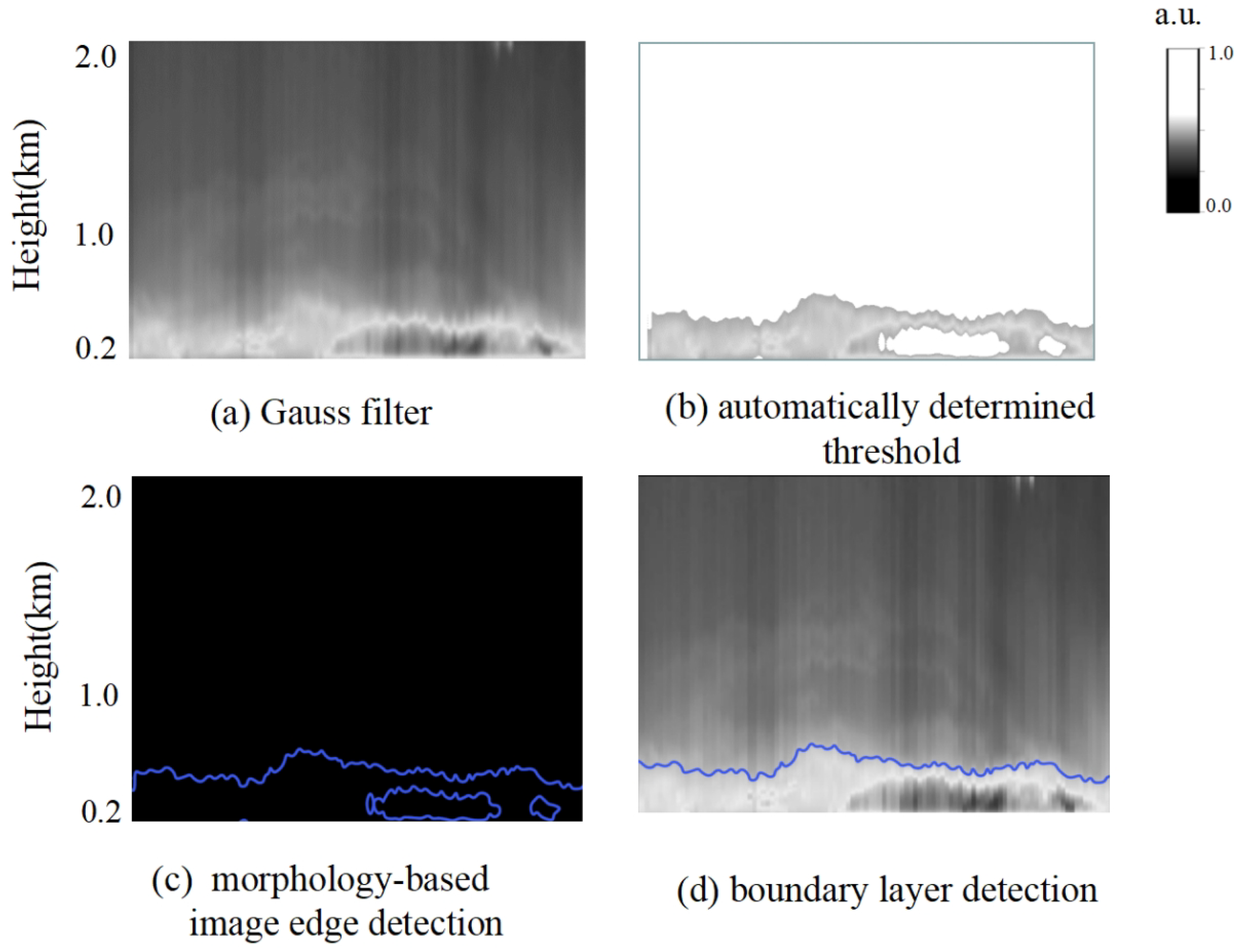
3. Methods for BLH Detection

Prior to determining the BLH, the range-corrected backscatter profiles were averaged over time and height to eliminate noise-induced aberrations. When the BLH detection method is used, only that part of the backscatter signal with a sufficiently high SNR is evaluated. The vertical smoothing of ceilometer profiles was done by a moving average across 10 range gates (100 m) and 50 time steps (30 min). This smoothing clearly increases the SNR, while preserving characteristic structure of the profiles. More details about the SNR calculation can be found in [46]. When low SNR values are considered, the BLH determination may be tainted by noise-related backscatter profiles rather than atmospheric signals. This is accomplished through the data pre-processing procedure. Any spots in the backscatter profile with an SNR less than a specified value are ignored. Here, the height at which the transition to data points with SNR < 1 occurs is used as the SNR stop level SNR. The background representative value is calculated from the signal above the top 5 km of the aerosol profiles.
For the Image Edge Detection (IED) method, an extension of the gradient detection algorithm is utilized in this project to determine the BLH [47]. The image edge refers to the part of the image where the brightness changes significantly. Based on the floating-point algorithm, we calculate and inverse the range-corrected lidar signal (PRR) to the 256-order gray color bar. Then, we draw the gray image of the PRR and take this image as the original image of morphological edge detection.
The steps of IED in Figure 2 are as follows:
(1) Gaussian filtering (Figure 2a): Gaussian filtering can effectively maintain the image information by filtering the superimposed noise. According to the gray values of the pixels to be filtered and their neighborhood points, the weight value of the Gaussian filter is calculated using a fixed standard deviation of 0.5, with the filter width of 3. Then, the input image is convoluted with the two-dimensional Gaussian filter, and the result is taken as the output pixel value.
(2) Automatic determined threshold operation (Figure 2b): According to the difference in gray characteristics between the target area to be extracted and its background, the image is regarded as a combination of two types of regions with different gray levels (target area and background area). Therefore, the threshold value is important to determine the target area.
Initially, we use a double threshold value, which can only segment the bright area with a high gray value. The value also needs to be adjusted based on different graphs. Then, we adopt an automatically determined threshold value from the Halcon operator. Halcon is a complete set of standard machine vision algorithm packages developed by the German MVtec company (https://www.mvtec.com/doc/halcon/12/en/index.html, accessed on 3 December 2022). The segmentation algorithm from the Halcon operator automatically calculates the histogram of the gray value and extracts the minimum value from the histogram as the parameter of the threshold value. The pixels within this threshold range belong to the target area, while those not within this threshold range belong to the background area. Thus, the corresponding binary image is generated. Next, the binary image is multiplied with the original image. The pixel area of the original image corresponding to the gray level of 1 in the binary image is retained, while the one corresponding to the gray level of 0 is discarded. The image obtained from the operation is used as the input for the next step.
(3) Morphology-based image edge detection (Figure 2c): In this step, the morphological close operation is performed on the binary image obtained in step 2. The dilation is followed by an erosion, using the same 3 × 3 structuring element for both operations. It can enlarge the boundaries of target regions and shrink background regions without destructing the original boundary shape. Connecting the edge points of the boundary shape produced by the closing operator allows the whole edge of the image to be obtained.
(4) Boundary layer detection (Figure 2d): To make the detection more accurate and faster, the detection height is limited to below 2 km. Some isolated and unconnected edges are also eliminated manually. Finally, the actual value of the boundary layer can be obtained by simply calculating the position coordinates of the target edge in the image.
The IED method has an inherent uncertainty, and its sources are due to the gradient calculations, the set of the threshold value, and the quality of the attenuated backscatter profiles. Besides the guidelines for manual checks [21], we select the days with well-defined vertical structures without cloud screening, set a threshold value of 1 for SNR after spatial averaging, and utilize the automatically determined threshold to help IED perform faster and more accurately. In addition, the post-processing step takes into account multiple sources of information (e.g., edge, surface meteorological and radon information, synoptic conditions, and wind profiles from sodar) to minimize the uncertainty. After more than one month of observation, we found that the uncertainty of the ceilometer-IED-based BLH in this campaign is lower on cloud-free days than that on cloudy days.

4. Results and Discussion

During the whole observing period, the boundary layer was more dominated by the mixed marine airflow and presented typically diurnal characteristics. The prevalent mixed marine environment was only replaced with the continental source at the end of June (from 25 June to 28 June). However, this four-day period experienced an increase in the radon and aerosol concentration from Melbourne/East Victoria air flow transported to the Cape Grim. In the meantime, the boundary layer was shallow and stable compared to that under marine sources. Therefore, detailed results for two days (Event 1: 3 June 2019 and Event 2: 25 June 2019) are presented in this section. These two days are chosen because they (1) correlate to periods when different types of continental sources are recorded (marine and continental mixed airflow for Event 1 and pure continental airflow for Event 2) and (2) illustrate two distinct atmospheric conditions for BLH detection: the first exhibits the convective boundary layer condition, while the second shows the more stratified structure.

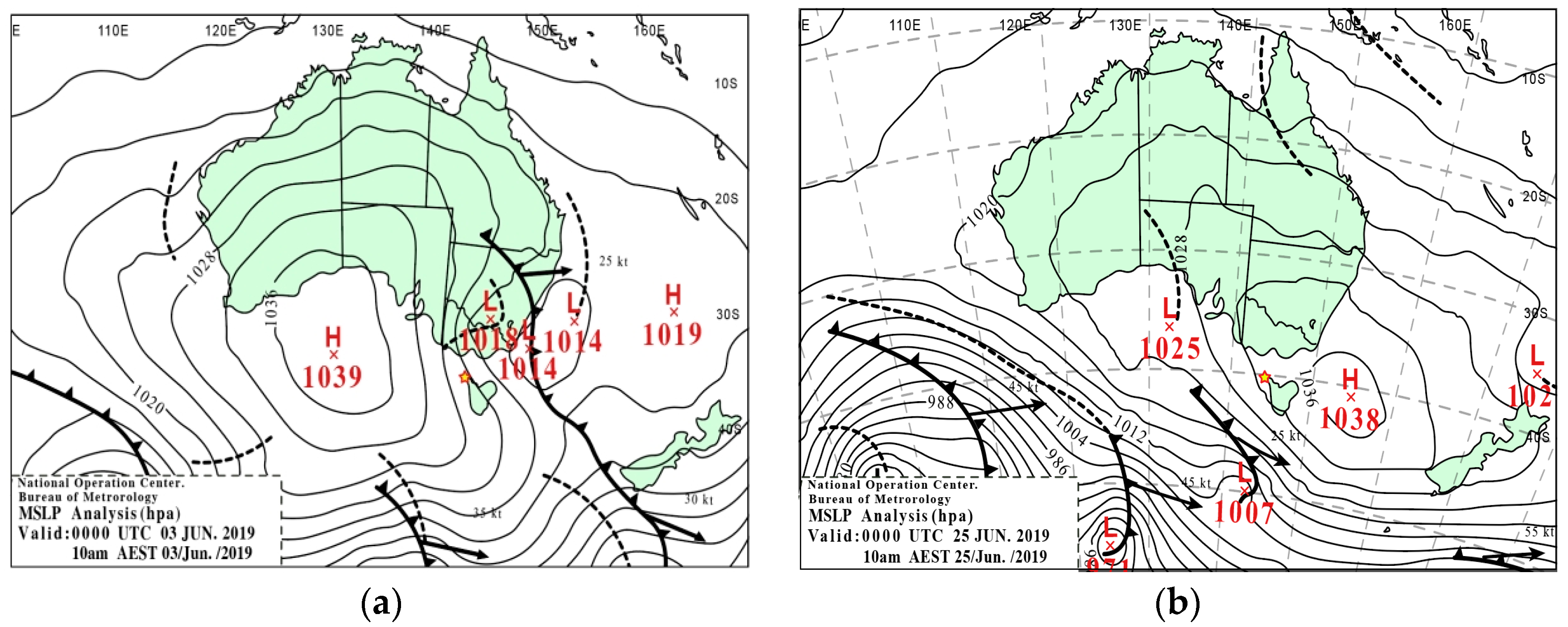
4.1. Synoptic Conditions

The synoptic pattern on 3 June 2019 (Event 1) consisted of a cyclone (low-pressure) system over the northern Tasmanian region. The associated anticyclone (high-pressure) system centered over the Indian Ocean was moving east (Figure 3a), which was found to be common, as the anticyclone density in winter showed a preference for migrating across the continent [48]. The temperature behind the new passage of cold front was cool. Compared to Event 1, a high pressure of 1036 hPa was on the site on 25 June 2019 (Figure 3b) in Event 2. The weakening of the primary anticyclone (1036 hPa) and the more distant cold front led to the rising temperatures and moderate winds on that day. It decays as a result of southeastward migration and the erosion by new stronger systems migrating from the southwest the next day (not shown here).

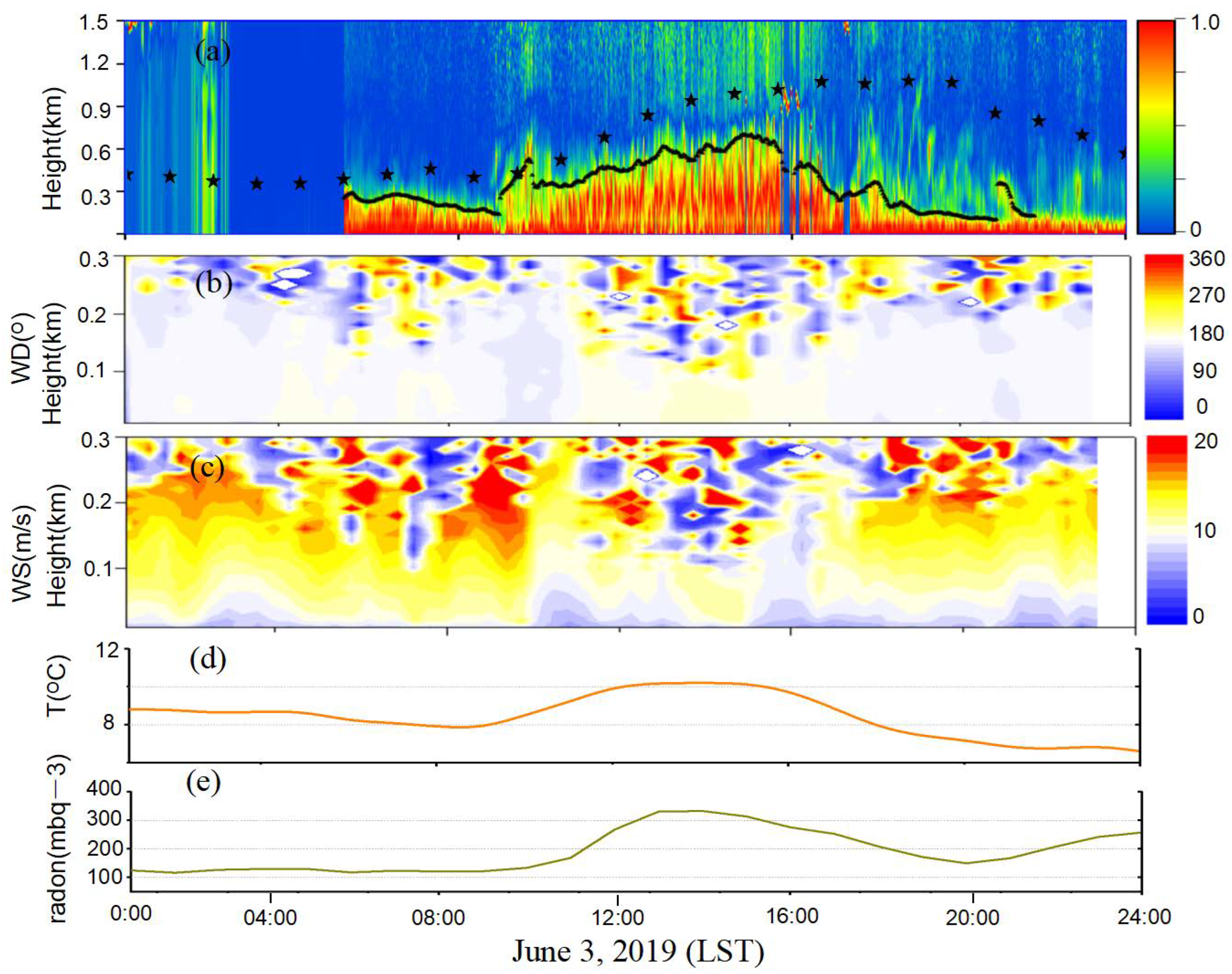
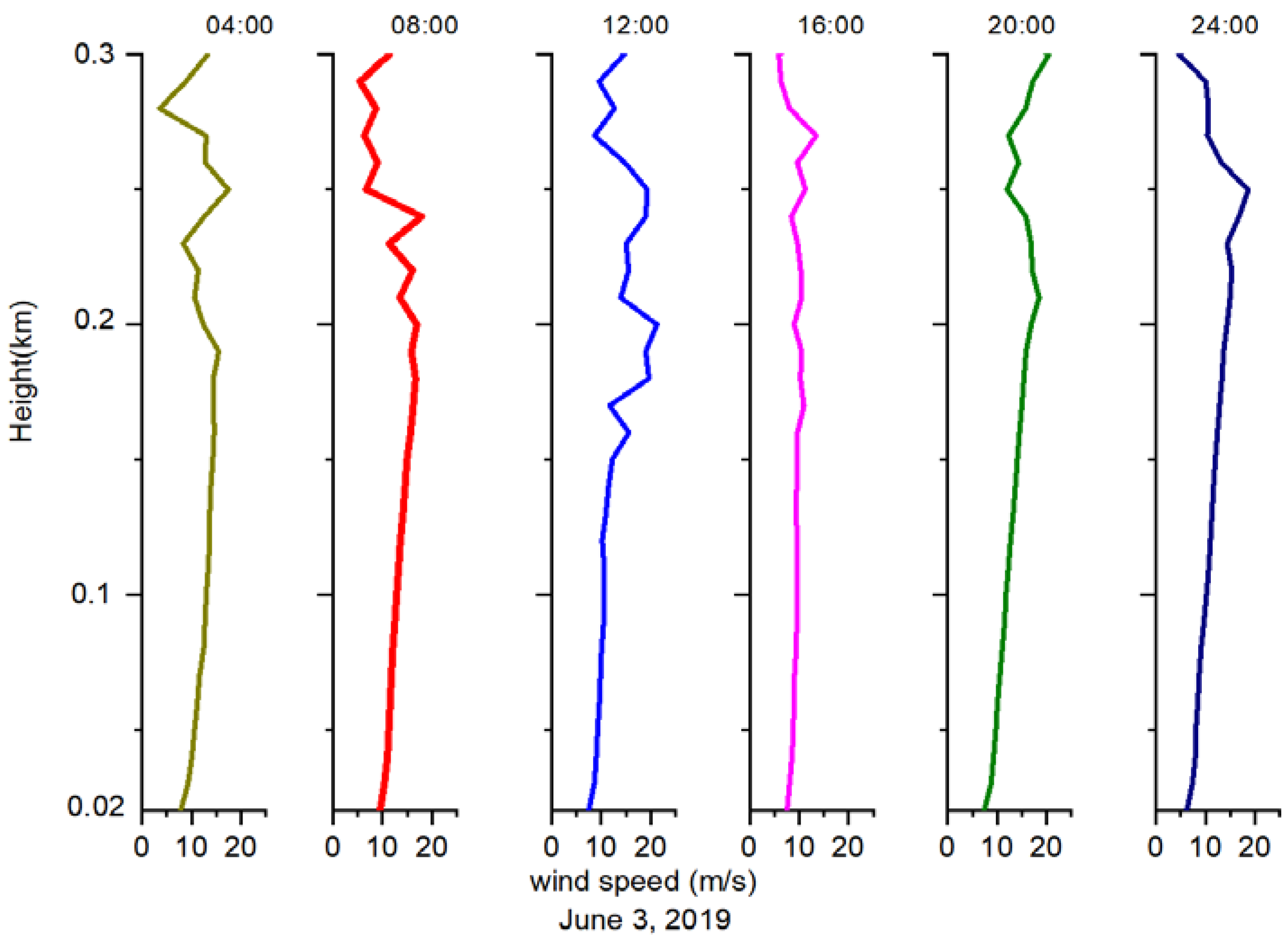
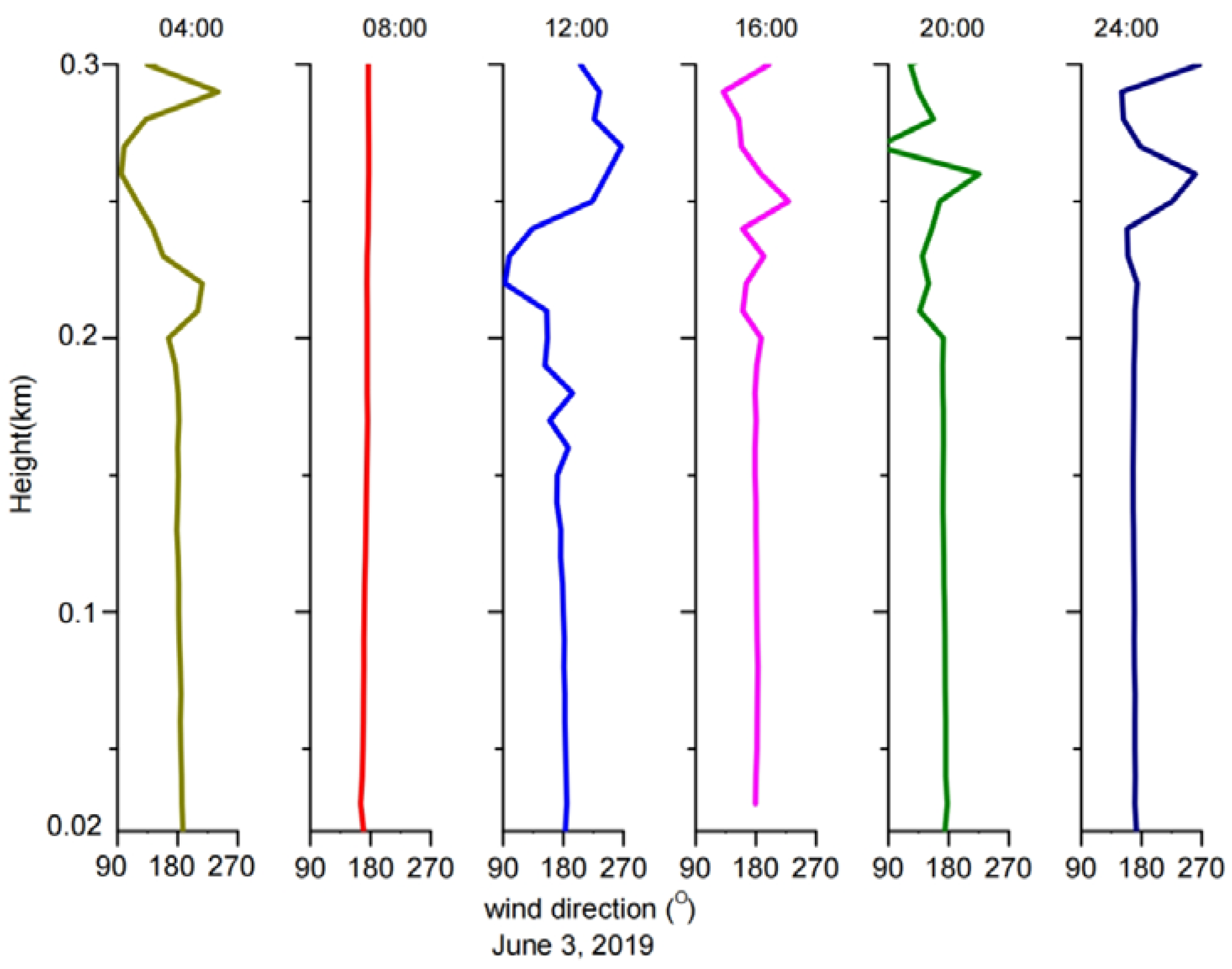
4.2. Event 1: 3 June 2019

The BLH on 3 June 2019 fluctuated between 200 m and 700 m (solid black line in Figure 4a), as measured by the attenuated backscatter data from the ceilometer. In the early morning (06:00–08:00 LST), the layer was stationary, whereas the BLH evolution became prominent during the convective period (09:00–16:00 LST), with an increasing growth rate (from ~20 to 110 mh−1), until it achieved its maximum height of 715 m at 15:20 LST. Then, the BLH decreased due to the reduced turbulence, with a nocturnal boundary layer (19:00–23:00 LST) at an averaged altitude of 123 m AGL. The correlation coefficient value of ERA5-BLH (black stars in Figure 4a) and ceilometer-BLH is 0.58. Generally, the ERA5 results overestimated the BLH (particularly in the afternoon), yielding a higher BLH ranging from 350 m to 1140 m. Similar comparisons are also found by Gu et al. [49]. One of the reasons for the discrepancy could be the coarse resolution of ERA5 reanalysis due to the topography [50,51]. Moreover, the notable overestimation of ERA5-BLH might be associated with the unstable activity in the lower troposphere that has not been adequately represented or simulated by the models used in reanalysis [52].
According to Figure 4b from the sodar, a nearly constant southern/southwestern wind is prevalent in the surface layer (20–100 m), whereas the direction above is variable. The sharp BLH increase occurs at 09:00 LST, when the southern winds accelerate significantly with the height seen in Figure 4c. More details about the wind profiles for this period will be analyzed in the next paragraph. Figure 4d shows the gradual increase in the temperature during the boundary layer growth period (09:00–16:00 LST). Simultaneously, the radon concentration in Figure 4e also began to increase, exhibiting the similar diurnal cycle seen in the boundary layer, which is characterized by an early afternoon maximum (330 mbqm−3 at 13:00 LST). Such correspondence indicates that the downward flow within the boundary layer may influence the near-surface radon concentration.
Figure 5 presents the 30 min averaged wind speed profiles from sodar on 3 June 2019. At the outset of the day (04:00–08:00 LST), the wind speed is rather steady from the surface to 215 m, where the BLH is quasi-stationary. From noon onward, the wind speed increases from a lower height of 170 m and reaches the maximum value of 21.2 ms−1 at 200 m. Later, the wind speed meanders again from 210 m up to 260 m until 16:00 LST, when the boundary layer begins to dissipate. The wind speed keeps constant from the surface to 300 m at 16:00 LST, suggesting that the strong vertical turbulent mixing makes the wind speed almost unchanged with height. Accordingly, the BLH decreases rapidly to 275 m at 17:00 LST and remains shallow at approximately 100 m (Figure 3a) afterward. From 20:00 LST to 24:00 LST, the increased wind speed gradient above 200 m, when radiative cooling tends to contain turbulent eddies vertically, is associated with the top of BLH at night.
Figure 6 shows the 30 min averaged wind direction profiles from sodar on 3 June 2019. At 04:00 LST, the wind is predominantly from the southern direction, except for the sudden counterclockwise turn from 220 m to 280 m (wind direction from 158.3° to 95.6°). It returns to the south at 08:00 LST and does not change with height. Then, it turns counterclockwise slightly up to 220 m, but sharply ascends in the opposite direction near midday (12:00 LST). The height at which the rate of direction (counterclockwise) is the greatest, i.e., 220 m, is related to the BLH when the boundary layer began to increase. From 16:00 LST, the wind turns clockwise at 210 m, and the highest veer is found between 260 m and 270 m. Such decoupling also marks the decrease in BLH. Later, at 20:00 LST, the direction profile keeps constant up to 200 m, supporting the increasing stability of the nocturnal boundary layer.
The calculated HYSPLIT back-trajectory frequency in Figure 7a shows that the air masses consist of two pathways: one passed through Tasmania, acquiring part of the continental aerosols, and the other from the baseline sector, with long-range transported soil or smoke. The sporadic fires in Figure 7b demonstrate that the continental-influenced air masses from Tasmania also contribute to the radon increase in the event.

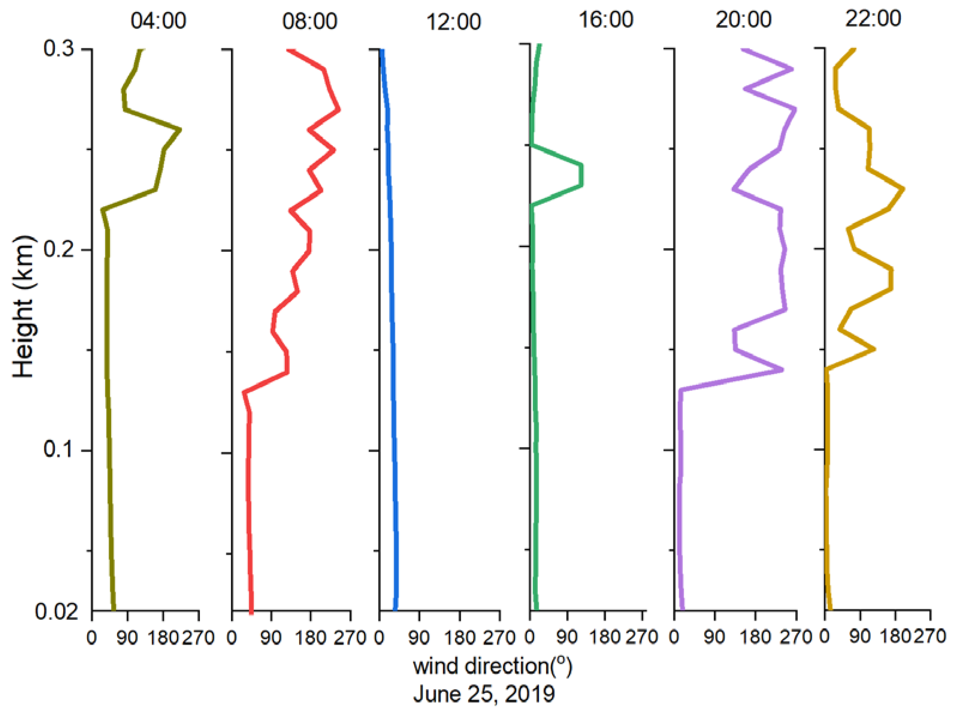
4.3. Event 2: 25 June 2019

Figure 8 exemplifies the homogeneous and stationary flow conditions on 25 June 2019. Compared to Event 1, the ceilometer backscattered intensity is generally closer to the surface (Figure 8a), with an averaged BLH of 362 ± 57 m. The ERA5 reveals a much better correlation coefficient value of 0.89 with ceilometer-BLH, except for a slightly higher BLH when the wind direction shifted from north/northwest to the northeast winds at all heights (10:00 LST to 15:00 LST). It is reasonable that the ERA5 performs better when the boundary layer is stable and less mixed, especially when the generalized boundary layer parameterization schemes in models are more related to a stable boundary layer [53]. This day was dominated by the northern/northeast winds below 100 m, while the higher level featured variable western winds (Figure 8b). The Melbourne/East Victoria air introduces more continental aerosols into the atmosphere via turbulence, resulting in a less mixed and shallower BLH (the minimum value of 226 m at 11:30 LST). The wind speed still increases with height constantly, but with moderate values (9–10 m/s) in Figure 8c. In general, the stable boundary layer is characterized by low turbulence and, therefore, small fluxes. It also brings a notable increase in high radon concentration, seen in Figure 8e. Specifically, the averaged radon concentration in Figure 8e reached to 2557 mbqm−3, nearly 10 times the value in case 1 (258 mbqm−3 on 3 June). It plummets from 2262 mbqm−3 at 15:00 LST (when the lower part of the boundary layer wind direction veers to the northeast) and increases in the next 8 hours, with the maximum value of 4224 mbqm−3 at 23:00 LST. The high radon observations through this day are reflective of the Melbourne/East Victoria land air mass sources. Furthermore, the stable boundary layer also contributes to the rise in the radon concentration.
Figure 9 shows the 30 min wind speed profiles from sodar on 25 June 2019. The profile is similar to case 1 (Figure 5). The wind speed is rather steady from the surface up to 210 m and becomes more meandering above at 04:00 LST. From noon to late afternoon (16:00 LST), the speed profiles maintain a constant moderate speed of 7.4 ± 0.8 m/s at all heights. Between 16:00 and 20:00 LST, the wind speed fluctuates again above 180 m, with an averaged value of 7.3 ± 2.6 m/s. In terms of the wind direction profiles in Figure 10, the northeast wind is generally prevailing to 120 m above the surface. The direction upward turns clockwise (from northeast to southeast) in the early morning (from 04:00 to 08:00 LST) and at night (from 20:00 to 22:00 LST). The stable wind in this period coincides with the minimum BLH of 226 m at 11:20 LST (Figure 8a). The veering of the wind direction at higher heights is particularly noticeable when the wind shifts from the Melbourne/East Victoria continental (northeast: 2–18°) to the Tasmania continental direction (southeast: 125–169°) (Figure 8b). Therefore, the combination of the 2 continental sources at different heights leads to the rise of the radon concentration from 16:00 LST (Figure 8e).
The back-trajectory frequency (Figure 11a) travels mainly from Melbourne/East Victoria before approaching the observing site on 25 June. The peak radon concentration is attributed to the potentially wind-related artifacts due to scattering or re-suspended soil. The increased burning from prescribed burns or other heaters in Figure 11b also leads to the high radon concentration on 25 June.
Combining our 2 cases, we found that the wind (both speed and direction) profiles are generally split vertically into 2 regions: steady conditions in the relatively lower height (20–200 m) and variable conditions in the higher levels (200–300 m). Similar to Stull’s observation of wind shears in the boundary layer, the unstable layers we observed are characterized by variable wind speed, which is also often accompanied by a rapid change in wind direction. In addition, the highly turbulent wind flow above 200 m indicates that the wind loads acting on the boundary layer are significantly influenced by the approaching turbulent flow characteristics and then interact with the boundary layer. For example, the wind speeds under the Baseline Sector sources on 3 June are found to be stronger (10–18 m/s) in the daytime (above 200 m) compared to that on 25 June, because of the increased baroclinic with the new passage of the cold front. This fast wind develops within the boundary layer and contributes to the convective boundary layer growth acceleration. Furthermore, the maximum wind speed (21.2 m/s) is found at noon at 200 m on 3 June due to the enhanced mixing. Then, 3 hours later, the BLH peak (715 m) occurred at 15:20 LST. In comparison, the moderate winds and thermal inversion under the influence of the Melbourne/East Victoria continental source in case 2 (25 June) led to weaker heat flux. More detailed explanation about the shallow boundary under continental sources can be found in the Discussion.

5. Discussion: BLH Estimations under Different Sources

In order to clarify the wind influences on the BLH in the Cape Grim, the observing period is statistically examined under different sources, as shown in Figure 12. The white rectangle and the white circle in the box show the mean and median values, and the upper and lower edges in the white box represent the upper and lower points in the data set. The distribution of observable numerical points is presented on the left half.
From Figure 12a, the BLH under the northern winds is generally lower than that under the southern winds. For example, Melbourne/East Victoria continental source (0–60°) brings the minimum BLH averaged value of 515 ± 340 m, and the Western Australia transportation source (300–360°) leads to the value of 586 ± 267 m. It is worth noting that the Melbourne/East Victoria continental flow induces lower BLH than the Western Australia transportation flow. In comparison, the BLH under southern winds, such as the Baseline Sector marine source (190–280°) and the Northern Tasmania continental (120–180°) source, is higher at 730 ± 305 m and 726 ± 386 m, respectively. The maximum BLH value is observed under the Baseline Sector source with more marine aerosols. In summary, the boundary layer exhibits lower BLH under continental sources than that under marine sources. That is probably because the north/northeasterly winds (continental sources) advected cold land air masses and led to the formation of a thermal internal boundary layer. Such thermal inversion reduces the turbulence and, hence, results in lower BLH under continental sources. Especially the Melbourne/East Victoria continental source in case 2 may contain absorption aerosols (considering the fire spots in Figure 11). The upper level of BLH warming by these absorbing aerosols (i.e., black carbon) further stabilize the boundary layer and weaken turbulence mixing, leading to a decrease in the BLH (Ding et al., 2016; Li et al., 2017). All these factors contribute to the shallower boundary layer under continental sources. In addition, the wind speed shows a positive relationship with the BLH values in Figure 12b. Specifically, the mean value of BLH under the wind speed 5 m/s, 5–10 m/s, 10–15 m/s, and >15 m/s are 561 ± 299 m, 612 ± 268 m, 906 ± 371 m, and 1130 ± 164 m, respectively.

6. Conclusions

To investigate the BLH evolution and its interaction with wind near the coast, we conducted ceilometer and sodar measurements in Cape Grim, located in the northwest of Tasmania, Australia, from 1 June 2019 to 13 July 2019. The BLH obtained from the ceilometer was validated against the wind conditions from sodar and compared with ECMWF ERA5 reanalysis data. The BLH in Cape Grim during the winter is on the order of 200–700 m. Compared to ceilometer-BLH, ERA5-BLH is generally positively biased. However, the BLH disparities between the ceilometer and ERA5 are small when the boundary layer is stable.
The BLH under different sources has a large variation range. The averaged BLH under marine sources is higher than that under continental sources. Owing to the observing site located at the height of a cliff (94 m) above mean sea level, the boundary layer we observed suffers less coastal impact than pure coastal sites in the westerly sector baseline. For example, considering the low BLH (confined to less than 700 m), the decoupling trend of the marine boundary layer [54] was not observed during the campaign. Furthermore, the boundary layer near the coast was characterized with a typical diurnal structure under the mixture of marine and continental sources, which is similar to the boundary layer evolution over land. The growth of the convective boundary layer was also highly associated with the changes in surface temperature and wind speed profiles, because the source of the turbulence in the convective boundary layer is the flux of buoyancy originated from the surface. In addition, the boundary layer in the coastal region is also sensitive to the wind field. The wind acceleration leads to the turbulent transport of momentum associated with increased instability [55]. In contrast, the boundary layer tends to be stable under pure continental sources. Hence, we think: (1) Cape Grim suffers less coastal impact than pure coastal sites, owing to the height of the cliff and its distance to the ocean; (2) The continental source could influence the boundary layer evolution in this one-month campaign in winter 2019. Especially the boundary layer tends to be shallower when the Melbourne/East Victorian continental source approaches.

Author Contributions

Z.C. wrote the manuscript and made the overall data analysis. R.S., S.C. and M.K. provided the raw data and relevant documents. Y.X. and Z.C. designed the IED algorithm for boundary layer height retrieval. A.G. helped improve the algorithm. The discussion with A.G.W., S.W. and A.G. is very valuable for the data analysis. The staff who assembled, tested, and calibrated the ceilometer and sodar systems are also acknowledged. All authors have read and agreed to the published version of the manuscript.

Funding

This research was funded by the Research Project Agreement “Cape Grim Boundary Layer Characterization Study” between the University of Melbourne and CSIRO. And the APC was funded by the Key Lab. of Environmental Optics and Technology, CAS (2005DP173065-2021-07). The authors gratefully acknowledge the effective cooperation of colleagues of Melbourne University and CSIRO. The Cape Grim Baseline Air Pollution Station is funded and managed by the Australian Bureau of Meteorology, and the AGAGE scientific program is jointly supervised with CSIRO Oceans and Atmosphere. Zhenyi Chen was also supported by the funding from the Key Lab. of Environmental Optics and Technology, CAS (2005DP173065-2021-07). The authors gratefully acknowledge the NOAA Air Resources Laboratory (ARL) for providing the HYSPLIT transport and dispersion model used in this research.

Data Availability Statement

Ceilometer and sodar data are available upon request to Melita Keywood at CSIRO.

Conflicts of Interest

The authors declare no conflict of interest.

References

  1. Stull, R.B. An Introduction to Boundary Layer Meteorology; Kluwer Academic Publishers: Norwell, MA, USA, 1988. [Google Scholar]
  2. Seaman, N.L. Meteorological modeling for air-quality assessments. Atmos. Environ. 2000, 34, 2231–2259. [Google Scholar] [CrossRef]
  3. Skamarock, W.C.; Klemp, J.B.; Dudhia, J.; Gill, D.O.; Barker, D.M.; Duda, M.G.; Huang, X.Y.; Wang, W.; Powers, J.G. A description of the advanced research WRF Version 3. NCAR Tech. Note 2008, 125, 1–3. [Google Scholar]
  4. Peña, A.; Gryning, S.E.; Hahmann, A.N. Observations of the atmospheric boundary layer height under marine upstream flow conditions at a coastal site. J. Geophys. Res. 2013, 118, 1924–1940. [Google Scholar] [CrossRef]
  5. Mace, G.G.; Protat, A. Clouds over the Southern Ocean as Observed from the R/V Investigator during CAPRICORN. Part II: The Properties of Nonprecipitating Stratocumulus. J. Appl. Meteorol. Clim. 2018, 57, 1805–1823. [Google Scholar] [CrossRef]
  6. Welton, E.J.; Voss, K.J.; Gordon, H.R.; Maring, H.; Smirnov, A.; Holben, B.; Schmid, B.; Livingston, J.M.; Russell, P.B.; Durkee, P.A.; et al. Ground-based lidar measurements of aerosols during ACE-2: Instrument description, results, and comparisons with other ground-based and airborne measurements. Tellus B 2000, 52, 636–651. [Google Scholar] [CrossRef] [Green Version]
  7. Emeis, S.; Schäfer, K.; Münkel, C. Observation of the structure of the urban boundary layer with different ceilometers and validation by RASS data. Meteorol. Z. 2009, 18, 149–154. [Google Scholar] [CrossRef]
  8. Groß, S.; Tesche, M.; Freudenthaler, V.; Toledano, C.; Wiegner, M.; Ansmann, A.; Althausen, D.; Seefeldner, M. Characterization of Saharan dust, marine aerosols and mixtures of biomass-burning aerosols and dust by means of multi-wavelength depolarization and Raman lidar measurements during SAMUM 2. Tellus B 2011, 63, 706–724. [Google Scholar] [CrossRef]
  9. Bravo-Aranda, J.A.; Moreira, G.A.; Navas-Guzman Granados-Munoz, M.J.; Gurrero-Rascado, J.L.; Pozo-Vazquez, D.; Arbizu-Barrena, C.; Reyes, F.J.O.; Mallet, M.; Arboledas, L.A. A new methodology for PBL height estimations based on lidar depolarization measurements: Analysis and comparison against NWR and WRF model-based results. Atmos. Chem. Phys. 2017, 17, 6839–6851. [Google Scholar] [CrossRef] [Green Version]
  10. Su, T.; Li, J.; Li, C.; Xiang, P.; Lau, A.K.-H.; Guo, J.; Yang, D.; Miao, Y. An intercomparison of long-term planetary boundary layer heights retrieved from CALIPSO, ground-based lidar, and radiosonde measurements over Hong Kong. J. Geophys. Res. Atmos. 2017, 122, 3929–3943. [Google Scholar] [CrossRef]
  11. Alexander, S.P.; Protat, A. Vertical profiling of aerosols with a combined raman-elastic backscatter lidar in the remote Southern Ocean marine boundary layer (43–66° S, 132–150° E). J. Geophys. Res. 2019, 124, 12107–12125. [Google Scholar] [CrossRef]
  12. Tangborn, A.; Demoz, B.; Carroll, B.J.; Santanello, J.; Anderson, J.L. Assimilation of lidar planetary boundary layer height observations. Atmos. Meas. Tech. 2021, 14, 1009–1110. [Google Scholar] [CrossRef]
  13. Duenas, C.; Perez, M.; Fernandez, M.C.; Carretero, J. Radon concentrations in surface air and vertical atmospheric stability of the lower atmosphere. J Environ. Radioact. 1996, 31, 87–102. [Google Scholar] [CrossRef]
  14. Salzano, R.; Pasini, A.; Casasanta, G.; Cacciani, G.; Perrino, C. Quantitative Interpretation of Air Radon Progeny Fluctuations in Terms of Stability Conditions in the Atmospheric Boundary Layer. Bound.-Layer Meteorol. 2016, 160, 529–550. [Google Scholar] [CrossRef]
  15. Crawford, J.; Chambers, S.D.; Williams, A.G. Assessing the impact of synoptic weather systems on air quality in Sydney using Radon 222. Atmos. Environ. 2022, 295, 119537. [Google Scholar] [CrossRef]
  16. Sesana, L.; Caprioli, E.; Marcazzan, G.M. Long period study of outdoor radon concentration in Milan and correlation between its temporal variations and dispersion properties of atmosphere. J. Environ. Radioact. 2003, 65, 147–160. [Google Scholar] [CrossRef]
  17. Keller, C.A.; Huwald, H.; Vollmer, M.K.; Wenger, A.; Hill, M.; Parlange, M.B.; Reimannet, S. Fiber optic distributed temperature sensing for the determination of the nocturnal atmospheric boundary layer height. Atmos. Meas. Tech. 2011, 4, 143–149. [Google Scholar] [CrossRef] [Green Version]
  18. Vecchi, R.; Piziali, F.A.; Valli, G.; Favaron, M.; Bernardoni, V. Radon-based estimates of equivalent mixing layer heights. Atmos. Environ. 2019, 197, 150–158. [Google Scholar] [CrossRef]
  19. Emeis, S.; Schäfer, K.; Münkel, C.; Friedl, R.; Suppan, P. Evaluation of the interpretation of ceilometer data with RASS and radiosonde data. Bound.-Layer Meteorol. 2012, 143, 25–35. [Google Scholar] [CrossRef]
  20. Pichelli, E.; Ferretti, R.; Cacciani MSiani, A.M.; Ciardini, V.; Iorio, T.D. The role of urban boundary layer investigated with high-resolution models and ground-based observations in Rome area: A step towards understanding parameterization potentialities. Atmos. Meas. Tech. 2014, 7, 315–332. [Google Scholar] [CrossRef] [Green Version]
  21. Poltera, Y.; Martucci, G.; Collaud Coen, M.; Hervo, M.; Emmenegger, L.; Henne, S.; Brunner, D.; Haefele, A. PathfinderTURB: An automatic boundary layer algorithm. Development, validation and application to study the impact on in situ measurements at the Jungfraujoch. Atmos. Chem. Phys. 2017, 17, 10051–10070. [Google Scholar] [CrossRef] [Green Version]
  22. Steyn, D.G.; Baldi, M.; Hoff, R.M. The detection of mixed layer depth and entrainment zone thickness from lidar backscatter profiles. J. Atmos. Ocean. Technol. 1999, 16, 953–959. [Google Scholar] [CrossRef]
  23. Flamant, C.; Pelon, J.; Flamant, P.H.; Durand, P. Lidar determination of the entrainement zone thickness at the top of the unstable marine atmospheric boundary-layer. Bound.-Layer Meteorol. 1997, 83, 247–284. [Google Scholar] [CrossRef]
  24. Baars, H.; Ansmann, A.; Engelmann, R.; Althausen, D. Continuous monitoring of the boundary-layer top with lidar. Atmos. Chem. Phys. 2008, 8, 7281–7296. [Google Scholar] [CrossRef] [Green Version]
  25. Chen, Z.Y.; Schofield, R.; Rayner, P.; Liu, C.; Vincent, C.; Fiddes, S.; Ryan, R.G.; Alroe, J.; Ristovski, Z.; Shu, X.W. Characterization of aerosols over the Great Barrier Reef: The influence of transported continental sources. Sci. Total Environ. 2019, 690, 426–437. [Google Scholar] [CrossRef]
  26. Hooper, W.P.; Florante, E.W. Lidar measurements of wind in the planetary boundary layer: The method, accuracy and results from joint measurements with radiosonde and kytoon. J. Clim. Appl. Meteor. 1986, 25, 990–1001. [Google Scholar] [CrossRef]
  27. Hennemuth, B.; Lammert, A. Determination of the atmospheric boundary layer height from radiosonde and lidar backscatter. Bound.-Layer Meteorol. 2006, 120, 181–200. [Google Scholar] [CrossRef]
  28. de Bruine, M.; Apituley, A.; Donovan, D.P.; Klein Baltink, H.; de Haij, M.J. Pathfinder: Applying graph theory to consistent tracking of daytime mixed layer height with backscatter lidar. Atmos. Meas. Tech. 2017, 10, 1893–1909. [Google Scholar] [CrossRef] [Green Version]
  29. Rieutord, T.; Aubert, S.; Machado, T. Deriving boundary layer height from aerosol lidar using machine learning: KABL and ADABL algorithms. Atmos. Meas. Tech. 2021, 14, 4335–4353. [Google Scholar] [CrossRef]
  30. Haeffelin, M.; Angelini, F.; Morille, Y.; Martucci, G.; Frey, S.; Gobbi, G.; Lolli, S.; O’dowd, C.; Sauvage, L.; Xueref-Rémy, I.; et al. Evaluation of mixing-height retrievals from automatic profiling lidars and ceilometers in view of future integrated networks in Europe. Bound.-Layer Meteorol. 2012, 143, 49–75. [Google Scholar] [CrossRef]
  31. Lewis, J.R.; Welton, E.J.; Molod, A.M.; Joseph, E. Improved boundary layer depth retrievals from MPLNET. J. Geophys. Res.-Atmos. 2013, 118, 9870–9879. [Google Scholar] [CrossRef]
  32. Vivone, G.; D’Amico, G.; Summa, D.; Lolli, S.; Amodeo, A.; Bortoli, D.; Pappalardo, G. Atmospheric boundary layer height estimation from aerosol lidar: A new approach based on morphological image processing techniques. Atmos. Chem. Phys. 2021, 21, 4249–4265. [Google Scholar] [CrossRef]
  33. Zahorowski, W.; Chambers, S.; Wang, T.; Kang, C.H.; Uno, I.; Poon, S.; Oh, S.N.; Werczynski, S.; Kim, J.; Henderson-Sellers, A.N.N. Radon-222 in boundary layer and free tropospheric continental outflow events at three ACE-Asia sites. Tellus B 2005, 57, 124–140. [Google Scholar] [CrossRef]
  34. Deardorff, J.W.; Willis, G.E.; Stockton, B.H. Laboratory studies of the entrainment zone of a convectively mixed layer. J. Fluid Mech. 1980, 100, 41–64. [Google Scholar] [CrossRef]
  35. Münkel, C.; Eresmaa, N.; Räsänen, J.; Karppinen, A. Retrieval of Mixing Height and Dust Concentration with Lidar Ceilometer. Bound.-Layer Meteorol. 2007, 124, 117–128. [Google Scholar] [CrossRef]
  36. Wiegner, M.; Gasteiger, J. Correction of water vapor absorption for aerosol remote sensing with ceilometers. Atmos. Meas. Tech. 2015, 8, 3971–3984. [Google Scholar] [CrossRef] [Green Version]
  37. Martucci, G.; Milroy, C.; O’Dowd, C.D. Detection of Cloud-Base Height Using Jenoptik CHM15K and Vaisala Ceilometers. J. Atmos. Ocean. Technol. 2010, 27, 305–318. [Google Scholar] [CrossRef]
  38. Tsaknakis, G.; Papayannis, A.; Kokkalis, P.; Amiridis, A.; Kambezidis, H.; Mamouri, R.; Georgoussis, G.; Advikos, G. Inter-comparison of Lidar and Ceilometer Retrievas for Aerosol and Planetary Boundary Layer Profiling over Athens, Greece. Atmos. Meas. Tech. 2011, 4, 1261–1273. [Google Scholar] [CrossRef] [Green Version]
  39. Wyngaard, J.C.; Lemone, M.A. Behavior of the refractive index structure parameter in the entraining convective boundary layer. J. Atmos. Sci. 1980, 37, 1573–1585. [Google Scholar] [CrossRef]
  40. Beyrich, F.; Gryning, S.E. Estimation of the entrainment zone depth in a shallow convective boundary layer from sodar data. J. Appl. Meteorol. 1998, 37, 255–268. [Google Scholar] [CrossRef]
  41. Helmis, C.G.; Flocas, H.A.; Kalogiros, J.A.; Asimakopoulos, D.N. Strong down slope winds and application of hydraulic-like theory. J. Geophys Res. Clim. Phys. Atmos. 2000, 105, 18039–18051. [Google Scholar] [CrossRef]
  42. Behrens, P.; Bradley, S.; Wiens, T. A multisodar approach to wind profiling. J. Atmos. Ocean. Technol. 2010, 27, 1165–1174. [Google Scholar] [CrossRef]
  43. Saha, S.; Sharma, S.; Kumar, K.N.; Kumar, P.; Lal, S.; Kamat, D. Investigation of Atmospheric Boundary Layer characteristics using Ceilometer Lidar, COSMIC GPS RO satellite, Radiosonde and ERA-5 reanalysis dataset over Western Indian Region. Atmos. Res. 2022, 268, 105999. [Google Scholar] [CrossRef]
  44. Palm, S.P.; Benedetti, A.; Spinhirne, J. Validation of ECMWF global forecast model parameters using GLAS atmospheric channel measurements. Geophys. Res. Lett. 2005, 32, L22S09. [Google Scholar] [CrossRef]
  45. Draxler, R.R.; Rolph, G.D. HYSPLIT (HYbrid Single-Particle Lagrangian Integrated Trajectory) Model Access via NOAA ARL READY Website (http://www.arl.noaa.gov/HYSPLIT.php); NOAA Air Resources Laboratory: College Park, MD, USA, 2013. [Google Scholar]
  46. Heese, B.; Flentje, H.; Althausen, D.; Ansmann, A.; Frey, S. Ceilometer lidar comparison: Backscatter coefficient retrieval and signal-to-noise ratio determination. Atmos. Meas. Tech. 2010, 3, 1763–1770. [Google Scholar] [CrossRef] [Green Version]
  47. Xiang, Y.; Zhang, T.S.; Liu, J.G.; Lv, L.H.; Dong, Y.S.; Chen, Z.Y. Atmosphere boundary layer height and its effect on air pollutants in Beijing during winter heavy pollution. Atmos. Res. 2019, 21, 305–316. [Google Scholar] [CrossRef]
  48. Jones, D.; Simmonds, I. A climatology of Southern Hemisphere anticyclones. Clim. Dyn. 1994, 10, 333–348. [Google Scholar] [CrossRef]
  49. Alapaty, K.; Pleim, J.E.; Raman SDNiyogi, S.; Byun, D.W. Simulation of atmospheric boundary layer processes using local- and nonlocal-closure schemes. J. Appl. Meteorol. 1997, 36, 214–223. [Google Scholar] [CrossRef]
  50. Madonna, F.; Summa, D.; Girolamo, P.D.; Marra, F.; Wang, Y.Z.; Rosoldi, M. Assessment of trends and uncertainties in the atmospheric boundary layer height estimated using radio sounding observations over Europe. Atmosphere 2021, 12, 301. [Google Scholar] [CrossRef]
  51. Guo, J.P.; Zhang, J.; Yang, H.L.; Zhang, S.D.; Huang, K.M.; Lv, Y.M.; Shao, J.; Yu, T.; Tong, B.; Li, J.; et al. Investigation of near-global daytime boundary layer height using high-resolution radiosondes: First results and comparison with ERA5, MERRA-2, JRA-55, and NCEP-2 reanalyses. Atmos. Chem. Phys. 2021, 21, 17079–17097. [Google Scholar] [CrossRef]
  52. Gu, J.; Zhang, Y.H.; Yang, N.; Wang, R. Comparisons in the global planetary boundary layer height obtained from COSMIC radio occultation, radiosonde, and reanalysis data. Atmos. Ocean. Sci. Lett. 2021, 14, 100018. [Google Scholar] [CrossRef]
  53. Luo, T.; Wang, Z.E.; Zhang, D.M.; Chen, B. Marine boundary layer structure as observed by A-train satellites. Atmos. Chem. Phys. 2016, 16, 5891–5903. [Google Scholar] [CrossRef]
  54. Busse, J.; Knupp, K. Observed Characteristics of the Afternoon-Evening Boundary Layer Transition Based on Sodar and Surface Data. J. Appl. Metrol. Clim. 2012, 51, 571–582. [Google Scholar] [CrossRef]
  55. Li, Z.Q.; Guo, J.P.; Ding, A.J.; Liao, H.; Liu, J.J.; Sun, Y.L.; Wang, T.J.; Xue, H.W.; Zhang, H.S.; Zhu, B. Aerosol and boundary-layer interactions and impact on air quality. Natl. Sci. Rev. 2017, 4, 810–833. [Google Scholar] [CrossRef]
Figure 1. (a) Map of observation site Cape Grim at northwestern Tasmania, Australia. (b) Potential sources of radon in the observing period.
Remotesensing 15 00461 g001
Figure 2. The processing steps of IED.
Remotesensing 15 00461 g002
Figure 3. Mean sea-level pressure (MSLP) analyses show a high-pressure system west of observing site (yellow star) on (a) 3 June 2019 and on (b) 25 June 2019. Data are from the Australia Bureau of Meteorology (http://www.bom.gov.au/australia/charts/archive/index.shtml, accessed on 8 May 2022).
Remotesensing 15 00461 g003
Figure 4. An example illustrating the retrieval of BLH using the ceilometer measurements obtained on 3 June 2019 over Cape Grim. (a) Time-height cross section of the range-squared corrected ceilometer signal intensity during the entire diurnal cycle. Black lines and black stars indicate the BLH estimations from the IED based on ceilometer and ERA5 reanalysis, respectively. Vertically aligned color bar (in linear scale) on the right indicates the intensity in arbitrary units. (b) Wind direction form sodar, (c) wind speed from sodar, (d) near-surface temperature, and (e) radon concentration.
Remotesensing 15 00461 g004
Figure 5. Wind speed profiles measured from sodar on 3 June 2019.
Remotesensing 15 00461 g005
Figure 6. Wind direction profiles measured from sodar on 3 June 2019.
Remotesensing 15 00461 g006
Figure 7. (a) 48 h backward trajectory frequency (500 m) arriving at Cape Grim site on 3 June 2019. The back trajectories were calculated using NOAA HYSPLIT 4.8 model. (b) The fire spots are from level 2 Terra/MODIS thermal anomalies/fire product (MOD14).
Remotesensing 15 00461 g007
Figure 8. Another example illustrating the retrieval of BLH using the ceilometer measurements obtained on 25 June 2019 over Cape Grim. (a) Time-height cross section of the range-squared corrected ceilometer signal intensity during the entire diurnal cycle. Black lines and black stars indicate the BLH estimations from the IED based on ceilometer and ERA5 reanalysis, respectively. Vertically aligned color bar (in linear scale) on the right indicates the intensity in arbitrary units. (b) Wind direction form sodar, (c) wind speed from sodar, (d) near-surface temperature, and (e) radon concentration.
Remotesensing 15 00461 g008
Figure 9. Wind speed profiles measured from sodar on 25 June 2019.
Remotesensing 15 00461 g009
Figure 10. Wind direction profiles measured from sodar on 25 June 2019.
Remotesensing 15 00461 g010
Figure 11. (a) 48 h backward trajectory frequency (500 m) arriving at Cape Grim site on 25 June 2019. The back trajectories were calculated using NOAA HYSPLIT 4.8 model. (b) The fire spots are from level 2 Terra/MODIS thermal anomalies/fire product (MOD14).
Remotesensing 15 00461 g011
Figure 12. (a) Statistical result of BLH (retrieved by IED from the ceilometer) under different sources—Melbourne/Eastern VIC (WD: 0–60°), Northern Tasmania (WD: 120–180°), Baseline Sector (WD: 190–280°) and Western Australia (WD: 300–360°), and (b) under different wind speeds. The white rectangle and the white circle in the box show the mean and median values, and the upper and lower edges in the white box represent the upper and lower points in the data set. The distribution of observable numerical points is presented on the left half.
Remotesensing 15 00461 g012aRemotesensing 15 00461 g012b
Disclaimer/Publisher’s Note: The statements, opinions and data contained in all publications are solely those of the individual author(s) and contributor(s) and not of MDPI and/or the editor(s). MDPI and/or the editor(s) disclaim responsibility for any injury to people or property resulting from any ideas, methods, instructions or products referred to in the content.

