1. Introduction
Change detection using multi-temporal remote sensing images is one of the most important applications of remote sensing technology [
1,
2,
3,
4]. Change detection analysis is applied for land use and land cover monitoring [
5,
6], natural disaster assessment, urban management [
7,
8,
9] and monitoring [
10,
11,
12].
Change detection techniques fall into two categories according to the existence of additional ground reference data: supervised methods and unsupervised methods [
13,
14]. Supervised methods require ground truth to be given for a big training dataset [
15], which is labor-intensive and time-consuming [
3,
16]. In this paper, we mainly focus on unsupervised change detection methods. Early unsupervised SAR image change detection methods are mainly traditional change detection methods based on probabilistic models, multi-resolution analysis and clustering methods. Rignot et al. [
17] assume multi-look SAR intensities to be gamma distribution and use image differencing method for change detection. Bruzzone et al. [
18] use Markov random fields to model the relationships between adjacent pixels. Bovolo et al. [
19] utilize stationary wavelet decomposition to extract the multi-resolution features. Aiazzi et al. [
20] extract change features based on information theory. Zhang et al. [
21] proposed a novel Contourlet fusion clustering algorithm for unsupervised change detection.
In the past decade, deep learning has made unprecedented development. Due to its powerful feature extraction ability, deep learning has been widely used in the field of SAR image change detection [
4,
13,
22,
23,
24,
25,
26]. Since the change detection data of SAR have fewer labels, methods based on semi-supervised learning and unsupervised learning have been widely used in the field of SAR change detection. In the field of semi-supervised learning, Wang et al. proposed a graph-based knowledge supplement network, which can suppress the adverse effects of noisy samples by adding discriminative information from a labeled dataset [
27]. Zhao et al. proposed a semi-supervised SAR image change detection method based on a siamese variational autoencoder [
28]. In the field of unsupervised change detection, since there are no labels, how to train a neural network becomes a key issue. At present, there are mainly two types of solutions, as shown in
Figure 1a,b. The first is to use the existing pre-training model and the model parameters are used for feature extraction without modification [
13]. The pretrained model is trained using external large datasets. Essentially, this method transfers the trained model on the semantic segmentation task to the change detection task. If the model is trained on an optical image dataset and the datasets to be tested are SAR images, image style transfer for SAR and optical images was considered [
16,
29]. The second method does not use any other dataset. Only two registered SAR images obtained at different times are needed. First, the pseudo-labels are generated using traditional methods, such as FCM clustering. Second, some reliable pseudo-labels are selected to train the neural network. Finally, the original images are inputted into the model and the change detection results are acquired [
4,
23,
24,
25,
30,
31], as shown in
Figure 1b. For example, Qu et al. [
31] proposed a dual-domain network (DDNet) using discrete cosine transform (DCT) for unsupervised SAR image change detection. Gao et al. [
25] proposed a siamese adaptive fusion network (SAFNet) for unsupervised change detection. The pseudo-labels of DDNet and SAFNet are generated by the hierarchical FCM algorithm [
32]. Each method yields good results [
25,
31].
However, both methods have their own shortcomings. With the first method, it is difficult to adaptively process various real data due to the fixed network parameters. For the second method, it is necessary to manually design the criteria for sample selection. These selected samples are used to train the model. This is computationally expensive due to the time-consuming training process before testing. Furthermore, nearly all unsupervised methods need image binarization. Saha et al. [
13] use the OTSU method for thresholding. Shen et al. [
23] and Qu et al. [
31] use the FCM method for pre-classification. Tang et al. [
33] generate pseudo labels using the expectation-maximization (EM) algorithm. However, the traditional thresholding methods cannot handle regions with very little change [
34].
This paper studies local change detection. We break up the image into small patches to test the performance of the method using only local information processing. Traditional segmentation methods may lead to many false alarms if only locally cropped images are processed. If the original images are cropped into small patches, the final change detection results will be very different from the results using full images. In order to solve this problem, in our previous work [
34], we proposed a novel thresholding method called histogram fitting error minimization (HFEM) for a little-changed area. After the thresholding using HFEM, conditional random fields (CRFs) are used to model the relationships between the neighborhood pixels. Finally, the small fragments are removed. The fragment removal procedure was called post-processing in our previous work [
34]. If the area of the fragment is less than a given value
, it will be removed; otherwise, it will be retained. This procedure has been proven to be a very effective way to improve accuracy [
31,
34,
35]. However,
needs to be set manually. If
is set too large, some truly changed area will be removed. If it is set too small, some larger false alarms will not be removed. Therefore, the post-processing procedure is essentially a supervised manual trial-and-error procedure (MTEP). As for the subject of image binarization, many excellent adaptive binarization methods have been proposed to replace MTEP [
1,
36,
37]. It is meaningful to find a processing method that is not based on manual settings to replace post-processing.
In summary, there are currently two problems. First, existing methods do not perform well for local region change detection. Second, in our previous work, accuracy improvement largely depended on the fragment removal procedure. In order to solve these two problems, we proposed a novel unsupervised change detection framework called HFEM-CNN. Different from the above two frameworks based on unsupervised deep learning, this paper proposes a new end-to-end deep learning-based unsupervised change detection method, as shown in
Figure 1c. This framework does not need to select training samples. The training and testing are carried out at the same time and it can also learn parameters adaptively. Compared to
Figure 1b, the three procedures, including sample selection, training and testing, are combined into one step: multi-objective learning. Compared to our previous work [
34], we use CNN to replace CRF and post-processing. The CNN-based method does not require manual setting of fragment size threshold. Although there are also some hyperparameters, such as the learning rate, momentum and the number of iterations, these three hyperparameters are the same as in [
38]. This shows that such a setting is satisfactory for different tasks. Furthermore, the change detection results are also improved compared to the combination of CRF and the fragment removal procedure. This framework has the ability to detect cropped regions. The proposed method outperforms previous methods on the task of change detection for locally cropped regions.
In general, the contributions of this paper can be summarized as follows:
- 1.
We first consider local change detection. Local change detection is a challenge for unsupervised change detection. We find that the proposed method has great advantages in local change detection.
- 2.
This paper proposes a novel unsupervised change detection framework called HFEM-CNN. This framework combines sample selection, training and testing into one step: multi-objective learning. The parameters of the network are learned adaptively. Compared with our previous work, the method proposed in this paper is more automatic. It does not require fragment removal as the post-processing to achieve decent results.
- 3.
The experiments are conducted on both whole images and cropped images. The encouraging results demonstrate that the proposed method is effective for the local change detection task.
It should be noted that the specific structure of the CNN is not our particular concern. In this work, we design a simple fully convolutional neural network (FCNN) for the experiments. It should be noted that the structure of FCNN is different from the famous FCN [
39]. To facilitate the distinction, we use FCNN to refer to the fully convolutional network designed in this paper. Furthermore, the classic Unet [
40] and PSPNet [
41] are also used for unsupervised learning. In this paper, HFEM-FCNN, HFEM-Unet and HFEM-PSPNet are collectively referred to as HFEM-CNNs. The experiments demonstrate that simple neural networks such as FCNN and Unet perform better in this situation. As for the HPF, there are also many specific forms of HPF, such as difference operator, Sobel operator and Laplace operator. This paper uses difference operators as the specific forms of HPF for its simple practicality.
This paper is organized into six sections.
Section 2 presents the definition of local change detection and the problem formulation of the proposed method.
Section 3 elaborates the proposed method. The Experimental results on real multi-temporal SAR images are reported in
Section 4, which also contains the experimental design and evaluation criteria. Discussions concerning the proposed method are presented in
Section 5. Finally, conclusions are drawn in
Section 6.
4. Experiment
In this section, we implement experiments to demonstrate the effectiveness of the proposed framework. First, we describe the datasets and the evaluation criteria used in this experiment. Then, the experiment design is specified. The detailed experimental results are displayed in the final parts. In this experiment, the weight coefficient
is set to
for water change detection and to
for building change detection. The number of convolution layers
L in
Figure 5 is set to 8. The difference operator is used as the high-pass filter, as shown in Equation (
15). The proposed method and DDNet method are implemented using Pytorch 1.11 and CUDA 11.3 on a single NVIDIA RTX 3090 GPU. The FCMMRF, PCA-kmeans and HFEMCRF are implemented using MATLAB R2022a on AMD Ryzen 9 5900X CPU. We choose the stochastic gradient descent (SGD) method as the optimizer. The learning rate is set to
and the momentum is set to
. The number of iterations is set to 200.
For comparison, we experimented with four contrasting methods, called DDNet [
31], SAFNet [
25], FCMMRF [
44] and HFEMCRF [
34]. All four contrasting methods use the fragment removal procedure as postprocessing. Generally speaking, the parameter
in the fragment removal procedure is generally set between 20 and 30.
is set to 20 in the public code of SAFNet [
25,
45] and DDNet [
31,
46]. In our previous work,
is set to 25 for HFEMCRF [
34]. In order to maintain uniformity, we set
to 20 for all four contrasting methods in this experiment. The implementation of the DDNet method is to use the code published by the original authors. The other methods we implemented ourselves according to the original papers. We test four HFENCNNs, including HFEM-Unet, HFEM-FCNN, HFEM-PSPNet and HFEM-PSPNet using pretrained backbone (HFEM-PSPNet-Pre).
4.1. Dataset Descriptions
We use three real SAR datasets in the experiment. The real datasets are Bern dataset, Ottawa dataset and Tongzhou dataset.
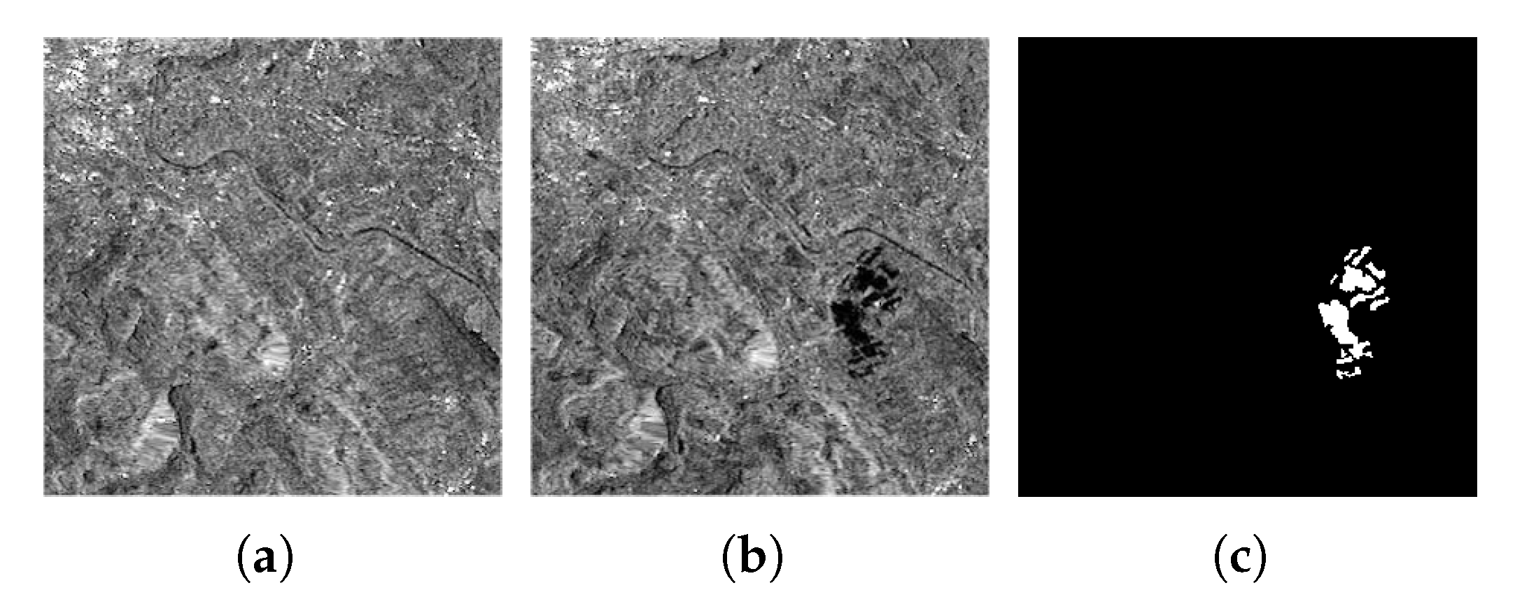
Bern dataset includes two
SAR images, which were acquired by the European Remote Sensing Satellite 2 (ERS 2) SAR satellite covering Bern city. The two images were acquired in April and May 1999. Between these two moments, the waters of the Aare River flooded parts of the cities of Thun and Bern, including Bern Airport. The two images of Bern dataset are illustrated in
Figure 8. The ground truth of Bern dataset is from [
1].
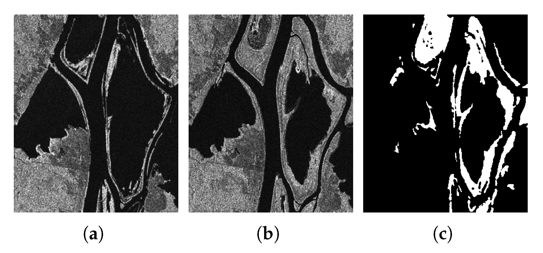
Ottawa dataset, which is shown in
Figure 9 was acquired by the RADARSAT SAR sensor in the Ottawa region. Two images (
) were acquired in May and August 1997, respectively. During this time, the area suffered from flooding. The ground truth of Ottawa dataset is from [
44].
Tongzhou dataset contains two SAR images acquired by TerraSAR-X. These two images are cropped from two large SAR amplitude images without multi-look operation, which means the range resolution is equivalent to
m and the azimuth resolution equals
m. The size of the cropped image is
. There were numerous newly built houses in this area between January 2014 and August 2015, so this dataset is used by us for building change detection. The ground truth of Tongzhou dataset is manually marked with reference to the optical images from Google Earth. However, two images of Tongzhou data are single-look images with greater speckle noise. Therefore, the multi-temporal SAR block-matching 3D (MSAR-BM3D) method [
47] is used to remove the speckle noise for Tongzhou dataset. The original and despeckled images of Tongzhou dataset are depicted in
Figure 10, respectively.
We did not perform despeckling on the Bern dataset and the Ottawa dataset because these two datasets are relatively less noisy. To illustrate this and also to evaluate the effect of despeckling, we select the homogeneous areas and calculate the equivalent number of looks (ENL) of each dataset. The
image of each dataset is selected to calculate the ENL. The selected patches of each image are shown in
Figure 11a–c. The selected patch of the original Tongzhou image is the same as that of the despeckled image. It can be seen from
Table 1 that the Bern dataset and the Ottawa dataset have relatively high ENL and do not require additional despeckling. However, two images of Tongzhou data are single-look images with greater speckle noise. Therefore, the multi-temporal SAR block-matching 3D (MSAR-BM3D) method [
47] is used to remove the speckle noise for Tongzhou dataset. The original and despeckled images of Tongzhou dataset are depicted in
Figure 10, respectively. The ENL of the despeckled image increased a lot, as shown in
Table 1.
4.2. Evaluation Criteria
The confusion matrix is used for the evaluation criteria. For binary classification problems, the size of the confusion matrix is
. The four elements in the confusion matrix are
,
,
,
. The definitions of these four variables are the same as [
34].
In this paper, we consider four evaluation criteria—overall accuracy (OA), precision, recall, mIOU and kappa coefficient (KC)—which are defined as follows:
The kappa coefficient is defined as follows:
where
4.3. Experimental Design
In this work, we implement real data experiments to demonstrate the effectiveness of our method. The real data experiment includes two parts. In the first part, the three whole datasets are used to demonstrate that the proposed method is suitable for whole datasets. The second part is the core part of the experiment. We randomly crop the raw images and labels. Each image is cropped into 20 small patches with size . The number of changes in the cropped area is very small. Experiments prove that our method is superior to other algorithms in this extreme case. The datasets in this experiment contain a total of 63 image pairs, of which the first three pairs of images are images of the complete data and the last 60 pairs are randomly cropped images. We use all 63 pairs of patches to perform the experiment in the second part. The purpose is to examine the algorithm’s average performance in various scenarios.
The method of the whole data and the cropped data experiments is shown in
Figure 12. The first line illustrates the experiment on whole datasets and the second line illustrates the experiment on the cropped datasets.
4.4. Experiment on Whole Datasets
In experiment 1, the datasets contain numerous changed pixels. The results of three whole datasets are shown in
Figure 13,
Figure 14 and
Figure 15. We can see that HFEM-PSPNet does not perform well in three datasets. PSPNet uses ResNet as the backbone. Since the ResNet network is relatively deep, the denoising ability of the model is too strong, so the output image is too smooth. Therefore, relatively shallow networks are better suited for unsupervised SAR change detection; previous research [
23,
31] also supports our view.
The numerical results of evaluation criteria are illustrated in
Table 2,
Table 3 and
Table 4. In this case, the traditional methods work well. The proposed method also obtains a good change detection performance. According to mIoU and the kappa coefficient, the proposed HFEM-FCNN performs the best on Bern dataset and Tongzhou dataset. However, from the three datasets, HFEM-CNNs did not show a significant advantage. The DDNet method performs the best on Ottawa dataset. Nonetheless, The accuracy of HFEM-CNNs is at the top of the three datasets. We do not prove that HFEM-CNNs are far superior to other methods on the whole datasets. We just need to prove that HFEM-CNNs can also achieve similar results with other excellent methods in ordinary cases. Experiment 1 aims to prove that HFEM-CNNs are suitable for normal datasets.
4.5. Experiment on Whole and Cropped Datasets
Both whole datasets and cropped datasets are used in experiment 2. The aim of experiment 2 is to test the overall performance of the algorithm in various situations. The total number of pairs of images is 63, including three whole datasets and 60 cropped datasets. In order to better evaluate the performance, We first calculate the mean value of each criterion, then we give visualized results of six selected different patches.
The mean values of numerical results are shown in
Table 5. The kappa coefficients of each dataset are shown in
Figure 16. The acronym ’WP’ means ’without post-processing’. The meaning of post-processing is fragment removal procedure, which is explained in
Section 1. The proposed method is compared with other methods, respectively. As can be seen from
Figure 16, HFEM-Unet and HFEM-FCNN are better than DDNet, FCMMRF and HFEMCRF. Even though HFEMCRF greatly improves accuracy through post-processing, the proposed HFEM-Unet is still 3.16 % higher than HFEMCRF in kappa coefficient and 2.87 % than in mIoU. If HFEMCRF has no post-processing, the performance of HFEM-CNNs is much stronger than that of HFEMCRF. Therefore, the proposed framework is a good substitute for CRF and fragment removal procedure.
For a subset of patches, our detection results have high kappa coefficients. However, for some special patches, the kappa coefficient value of HFEM-CNNs is very small. In order to visually demonstrate the effect of our method on different patches, we deliberately select eight patches. Four of them have good results and the results of the other four patches are not good. The indices of the four patches with good results are 8, 11, 30 and 43, respectively. The indices of the three patches with poor results are 23, 39 and 45, respectively.
Figure 17 illustrates the selected patches. The blue dots represent the patches with good results and the red dots represent the patches with poor results. We give the visualized results and analysis of these selected patches.
In our subsequent analysis, if there is no clear explanation, we use the row number in
Figure 18 or
Figure 19 to represent the patch number. For example, patch 1 in
Figure 18 represents the patch results shown in the first row in
Figure 18.
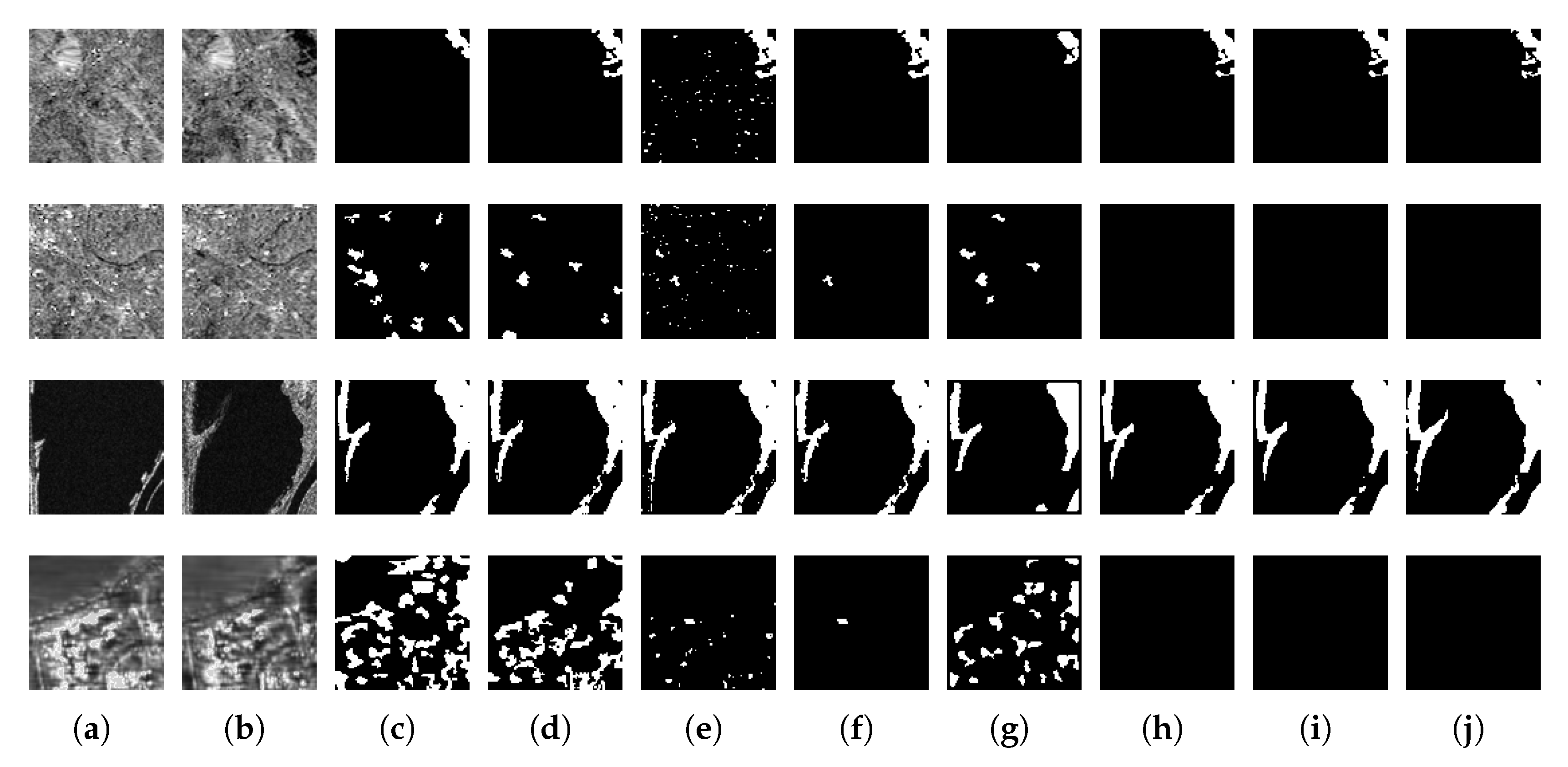
Figure 18 illustrates the results of four cropped patches with good results. Each line of
Figure 18 represents the data and detection results of a patch. Patch 1 and patch 2 are cropped from Bern dataset. Patch 3 is cropped from Ottawa dataset and Patch 4 is cropped from Tongzhou dataset. The selected patches include no change areas as well as changed areas. As can be seen from
Figure 18, for those patches with significant changes, our method performs well, as shown in patch 1 and patch 3 in
Figure 18. Not only our method, but nearly all methods also perform well on the patches with a lot of change. However, for those patches without change, such as patch 2 and patch 4 in
Figure 18, traditional methods do not perform well. The HFEM-CNN method can better avoid false alarms.
However, the proposed method can also lead to some unsatisfactory results, as shown in
Figure 19. We select three patches with poor results. From
Figure 19, we can clearly see that the proposed approach leaves out some of the details of the change. This is the reason for the low kappa coefficient in these patches. Nevertheless, from the effect point of view, our method greatly avoids false alarms at the cost of missing some details and we think it is still a good method. From the overall average kappa coefficient, the proposed method performs better than other methods. Due to the strong denoising ability of CNN, some tiny changes will be removed as noise.
5. Discussion
In this section, we first discuss the effect of random initialization. We do not fix the random seed and repeat the experiment 15 times. The hyperparameter is set to . These repeated experiments are intended to illustrate that the proposed method is less affected by randomness. Then, we discuss the influence of the hyperparameter , which aims to demonstrate the proposed method is robust with respect to the selection of the hyperparameter . The Unet is used as the CNN structure. Finally, we summarize the strengths and weaknesses of the proposed method.
5.1. The Effect of Random Initialization
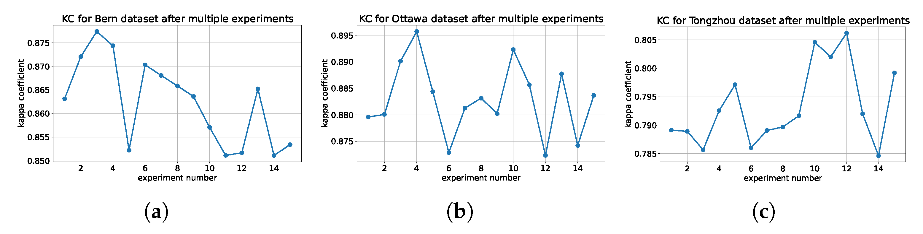
We set the same hyperparameter
and repeated experiments 15 times on the three datasets, respectively, to see how much performance is affected by randomness. The purpose of this experiment is to demonstrate that the performance of our method is reproducible and less affected by randomness. Let
R represent the difference between the maximum value and the minimum value of the kappa coefficient in multiple experiments. As we can see from
Figure 20, for Bern dataset,
, for Ottawa dataset,
, and for Tongzhou dataset,
. The values in
Table 2,
Table 3 and
Table 4 are the results of setting the random seed to 2022 for repeatability. Compared with the results in
Table 2,
Table 3 and
Table 4, the proposed method is relatively stable and less affected by randomness.
5.2. The Effect of
In the experiment, the weight coefficient
is set to
. If
is too large, the final output would be very close to HFEM. This means that the neighborhood information is not considered. In order to quantitatively discuss the influence of
, we show the effect of different lambdas on the final output using three whole datasets, as shown in
Figure 21. In order to ensure that the performance of the algorithm is not greatly affected by randomness, we do not fix the random seed. The performance shown in the
Table 2,
Table 3 and
Table 4 is one of the results of multiple experiments, so it is slightly different from the result in
Figure 21, but the error will not exceed one percent.
It can be seen from
Figure 21 that the setting of parameter
does affect the detection accuracy. Because of this, in the cropped data experiment, we uniformly set the parameter
to
for all cropped datasets. If
is too small, the output of the CNN will appear as an all-zero map. From the point of view of optimization, that the output is an all-zero map means
in Equation (
10) is approaching zero. Because of the small weight of
, the overall loss is mainly dominated by
. So it falls into a locally optimal solution.
Furthermore, as long as is set to about 2 to 3, the basic performance of the algorithm can still be guaranteed. We calculated the difference between the maximum and minimum kappa coefficients of the detection results when lambda equals . Let R denote the difference between the maximum value and the minimum value of the kappa coefficient using different . For Bern dataset, , for Ottawa dataset, and for Tongzhou dataset, . The difference is , and on Bern, Ottawa and Tongzhou datasets. Considering the impact of random initialization, the impact of changes in is even more negligible. For the Ottawa dataset, the influence of on the kappa coefficient is even lower than the influence of randomness on the kappa coefficient, which shows that the influence of lambda on the result is completely submerged in random noise. This shows that in such an interval, the effect of the method is relatively robust with respect to the selection of parameter .
Experiments prove that the proposed method is of great help in reducing false alarms. The proposed method has only one main hyperparameter . It can also be shown from the above two discussions that HFEM-Unet has little impact on random initialization. When is between 2 and 3, it has little impact on the final performance of the method. Therefore, HFEM-Unet is a relatively stable method that does not rely too much on hyperparameters. However, our previous work, HFEMCRF, is greatly affected by post-processing. Not only that, even if HFEMCRF uses post-processing, HFEM-CNN still slightly outperforms HFEMCRF on all 63 datasets. The proposed method is superior to HFEMCRF. Compared with the work of other scholars, such as DDNet, FCMMRF and SAFNet, the proposed method shows a great advantage in reducing the false alarm rate due to HFEM. However, the proposed method also has shortcomings. That is, the change detection of details needs to be improved. In order to reduce false alarms, the proposed method ignores some changes in details. This leads to the fact that the change detection results of the proposed method are not as good as other methods for some images with detailed changes.


