1. Introduction
Tides are one of the earliest aspects of oceanography to be recognized and applied in human activities [
1]. Tides, as a basic motion of seawater, are of great significance to research on water mass, ocean currents, storm surges and other ocean phenomena [
2]. The study of such seawater motions remains an important part of oceanography, with significant implications for coastal engineering and the exploitation of marine resources, especially in shallow seas. The Bohai and Yellow Seas (BYS) are marginal seas adjacent to China, where tides and tidal currents are rather strong and complicated. Based on observations and numerical models, the cotidal charts of the BYS have been constructed, revealing the basic characteristics of the main tidal constituents in the BYS [
3,
4,
5,
6], though quantitative improvement is still necessary.
The regional ocean models play an irreplaceable role in the investigation of tidal characteristics for the marginal seas. Numerical models of coastal ocean regions inevitably involve the treatment of open boundaries and, therefore, appropriate open boundary conditions (OBCs) must be applied [
7]. In regional ocean models, OBCs are essential for accurate simulation of tidal processes, and solutions in model interior are determined by the OBCs [
8]. In general, OBCs are obtained by interpolating the available observations near the open boundaries or deriving from larger scale models (e.g., the widely used TPXO tidal model data) through a nested grid approach [
9,
10]. In the case of lacking observations near the open boundary, significant uncertainties are introduced into the model by such interpolated or extrapolated boundary values [
11]. In practice, the model data may be inapplicable in terms of resolution and accuracy in shallow waters [
12], which means that manual adjustments need to be made empirically to obtain satisfactory simulation results [
13]. Adjoint method is widely implemented as a more advanced and powerful tool for the estimation of OBCs and other tidal parameters [
14,
15,
16,
17,
18].
Obtaining OBCs by adjoint methods also requires the support of observations. Tide gauge data are commonly used for tide studies; however, tide gauges are mainly located in shallow water, with a small number and uneven distribution [
19], which poses a challenge to the accuracy of regional tidal numerical research. The development of remote sensing technology has made up for this shortcoming, and satellite altimeter data cover a much larger area, including the open ocean, providing a great help to better study ocean tides [
20,
21]. In recent years, great development and progress has been made in altimeter instrumentation, processing algorithms and corrections, and products represented by X-TRACK have significantly improved the accuracy of altimeter data in coastal areas [
22]. The application of satellite altimeter data and products improves the inversion of tidal parameters by the adjoint method.
Satellite altimetry inevitably has some shortcomings. Different from the continuous and high-frequency sampling of tide gauge, the satellite altimeter data are limited by the orbit design, and the sampling rate is insufficient for ocean tides. Too long a sampling period at the same location will lead to tidal aliasing, which is not conducive to the study of ocean tides [
23]. The accuracy of measured altimeter data can be affected as the satellite approaches the coasts due to the contamination of signal by land [
24], which will lead to greater error in the altimeter data near the coast compared with that in the deep sea. In order to analyze tidal residuals in satellite data, gravity models of nontidal variability are required [
25], but there are certain technical defects in gravity recovery and climate experiments (GRACE) and gravity models [
26]. Accurate simulation of ocean tides serves as a correction for spaceborne measurements; it can be directly used for satellite altimetry data correction or indirectly used as GRACE or gravity field modeling [
23]. Therefore, more accurate numerical simulation of ocean tides also plays a significant role in the development of satellite altimetry.
In addition, the OBCs inversion with the adjoint method has been continuously optimized. In the original research, all points on the boundary were set as control parameters, which easily caused the ill-posedness of the inverse problem [
27,
28,
29]. For this problem, the independent points (IPs) scheme was proposed for optimization. With the help of IPs scheme, Lu and Zhang [
30] developed a two-dimensional (2D) tidal model and successfully inverted the bottom friction coefficients (BFCs). Since the interpolation is a core part of IPs scheme, the parameter settings of IPs selection and influence radius are constantly explored. Using a 2D tidal model, Cao et al. [
31] investigated the effect of different IP strategies on the inversion simulation results of OBCs in the BYS, indicating that using only two IPs can yield better simulated results. The IPs scheme has been applied to estimate OBCs, BFCs and other parameters in tide and internal tidal models [
32,
33,
34,
35]. In the above studies, linear interpolation was used in the IPs scheme, which would lead to non-smooth parameters of inversion. As an improvement, Pan et al. [
36] proposed to replace the Cressman interpolation (CI) with the spline interpolation (SI) to make inversed OBCs smoother and reduce the error of simulation results. Since then, IPs combined with SI have been continuously explored in the inversion of tidal parameters [
37,
38].
However, the location selection of IPs and influence radius are always unavoidable for IPs scheme when the method is applied to more general and open areas, a large number of sensitive experiments are required to obtain the best simulation results [
32]. For parameter estimation problems, it is of great importance to reduce the number of spatially varying control parameters due to the ill-posedness of the inverse problem [
35]. In this paper, trigonometric polynomials fitting (TPF) scheme is proposed to express the spatially varying OBCs and improve the estimation of OBCs in a 2D tidal model. The components of OBCs are expressed as a discrete Fourier series, and a finite number of trigonometric polynomials are used to construct OBCs, which reduces the number of control parameters. The BYS are selected as the computation domain; the more accurate and appropriate OBCs are estimated for regional tidal models by assimilating observations to optimize the coefficients of polynomials. The satellite altimeter data used for assimilation are also updated. Compared with previous studies, the data cover a wider time range and have higher accuracy, which can achieve more accurate tidal simulation. The IPs scheme is used as a comparison in the following experiments. Meanwhile, OBCs derived from data of ocean tidal models are used to perform numerical simulations to validate the inversion effect of TPF scheme.
This paper is organized as follows: the tidal model and derivation of the correction of parameters are shown in
Section 2. In
Section 3, twin experiments (TEs) are conducted to examine the feasibility and accuracy of TPF. In
Section 4, practical experiment (PE) is carried out in the BYS. The conclusion and summary are presented in
Section 5.
3. Twin Experiments
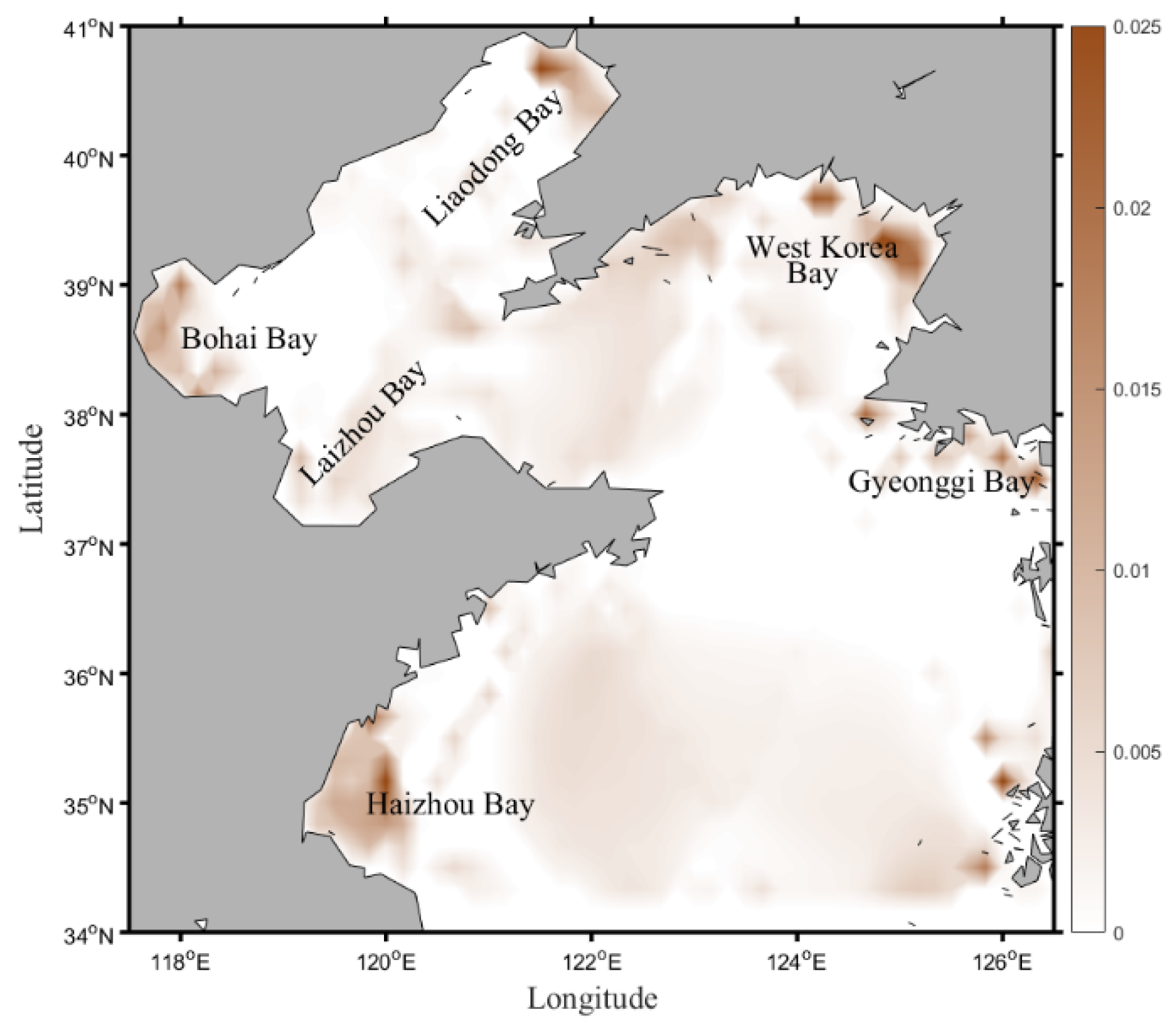
In this section, eight TEs are conducted to evaluate the feasibility and accuracy of the model and TPF scheme. Referring to Lu and Zhang [
38], the spatially varying BFCs (
Figure 3) are estimated by adjoint assimilation. The estimated BFCs in the major bays of the BYS are relatively large, which may be related to the local topography or formation of drag [
45,
46,
47]. The BFCs remain unchanged in the experiments and the eddy viscosity coefficient keeps constant during experiments.
3.1. Inversion Process
The process of TEs is listed as follows:
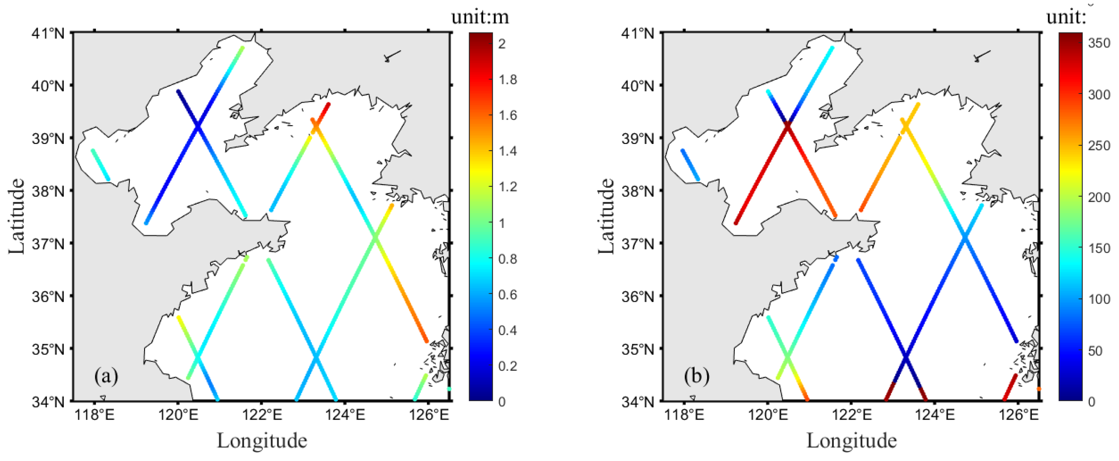
Step 1: The forward model is run with prescribed OBCs and BFCs (
Figure 3), and the simulated results on T/P-Jason altimeter tracks are chosen as “observations”.
Step 2: The FCs (the initial taken as zero here) of OBCs are used for running the forward model to obtain simulated water elevations.
Step 3: The difference in water elevations between simulated results from step 2 and “observations” in step 1 is used as the external drive to calculate the cost function.
Step 4: The gradients of the control parameters () are calculated by Equation (11), and then the control parameters are optimized by Equations (12)–(15).
Step 5: Optimized control parameters are assigned to new FCs of OBCs.
Steps 2–5 are repeated and the difference in water elevation simulation results and “observations” decreases. When a convergence criterion is met or the number of iteration steps reaches the specified number, the process of inversion terminates.
3.2. TEs Setting
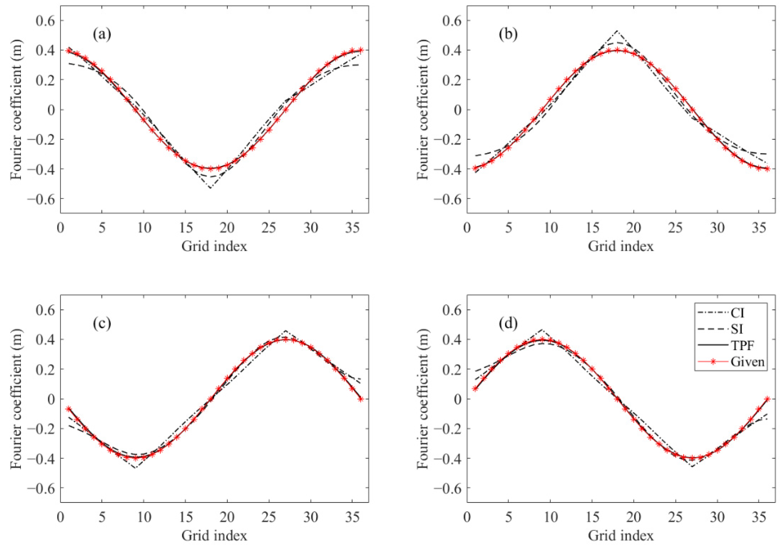
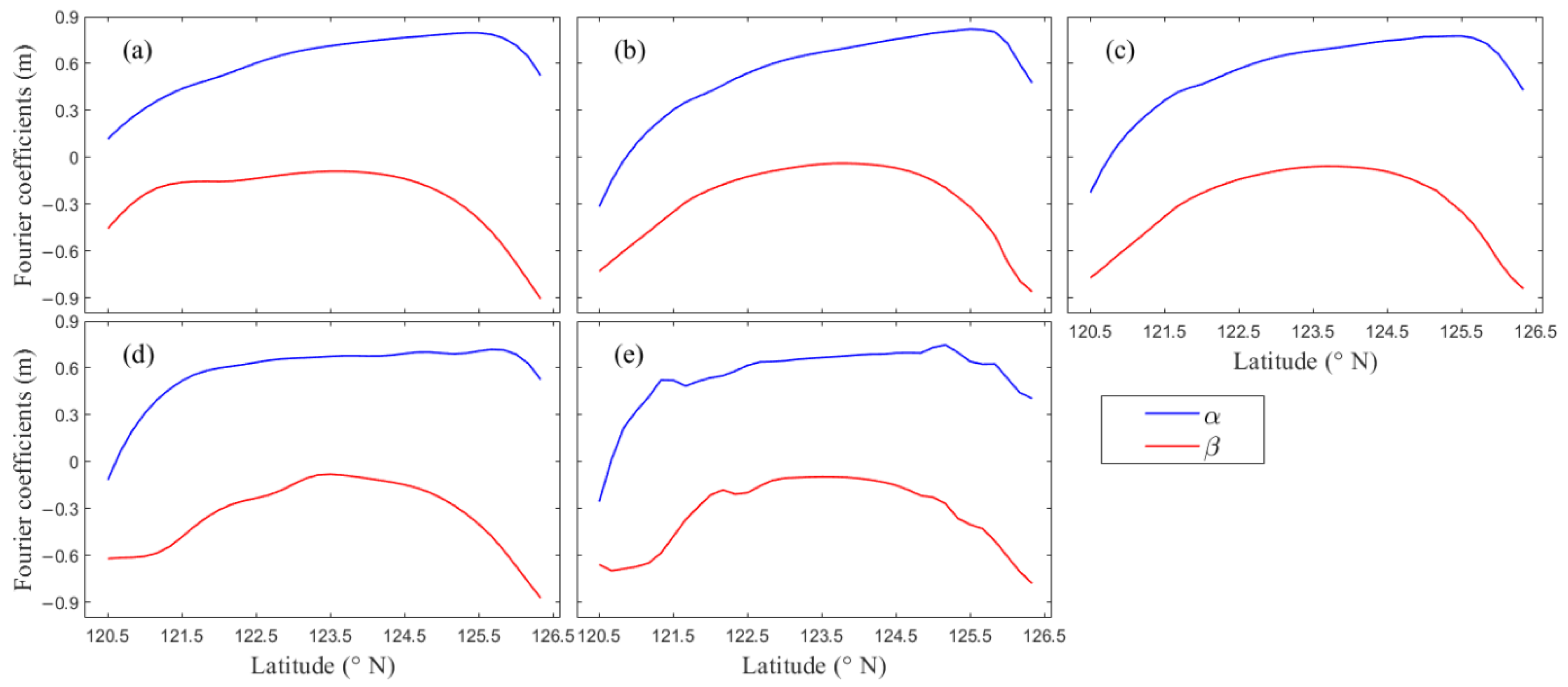
In TEs 1–4, four given FCs α are inverted, while β is set to be zero and does not participate in the inversion. Previous studies have shown that IPs schemes work best when the radius of influence is equal to the distance between IPs [
31,
36]. TEs setting is determined according to the basic research and preliminary experiments. The inversion process terminates when the number of iteration steps reaches 100. Several preliminary experiments were conducted to determine the number of IPs in IPs schemes and the maximum number of cycles in TPF scheme in different experiments. In TEs 1–4, for CI and SI schemes, five independent points are selected uniformly, and the MTP in TPF scheme is set to 1. The given and inverted FCs α are displayed in
Figure 4.
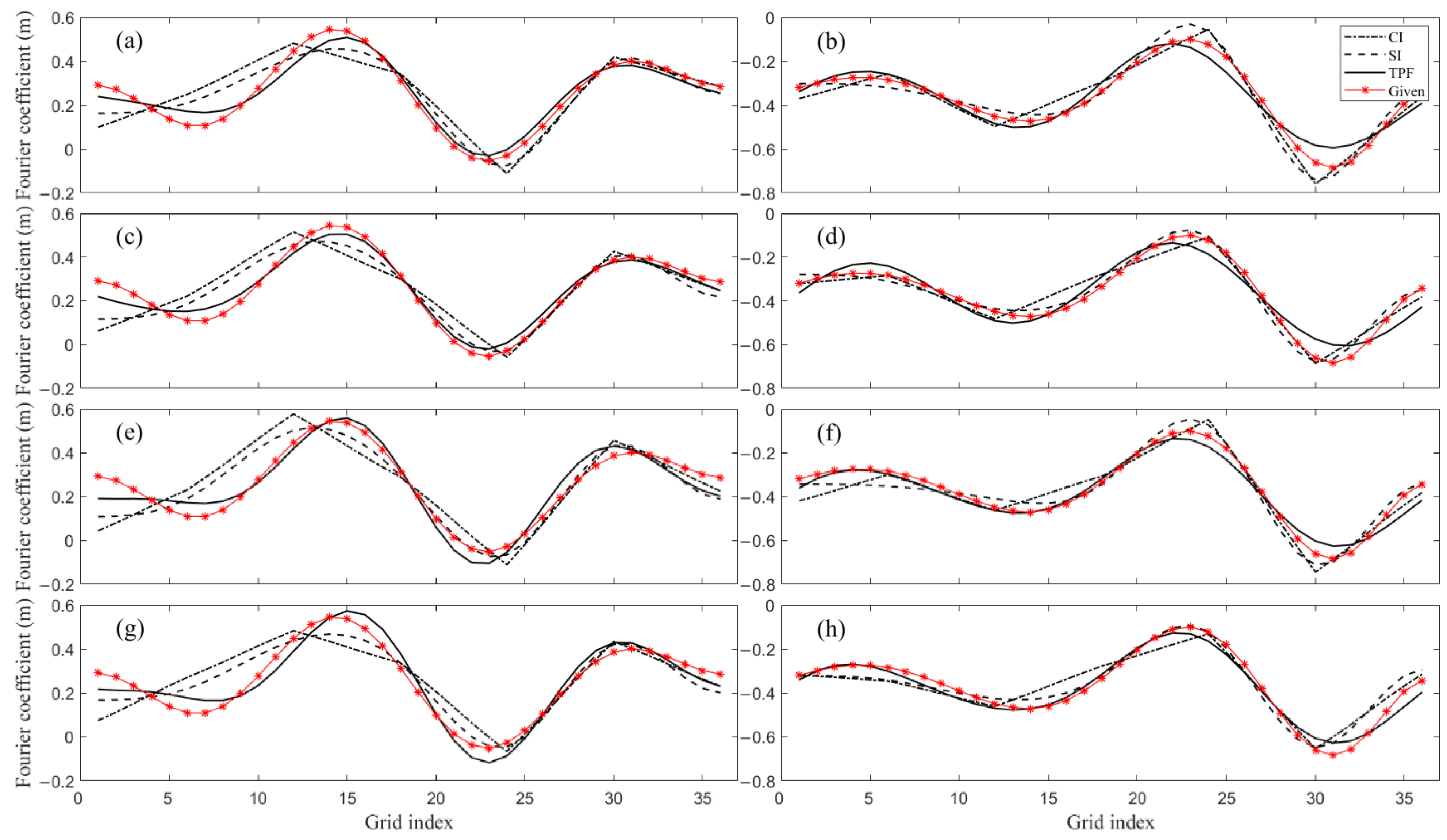
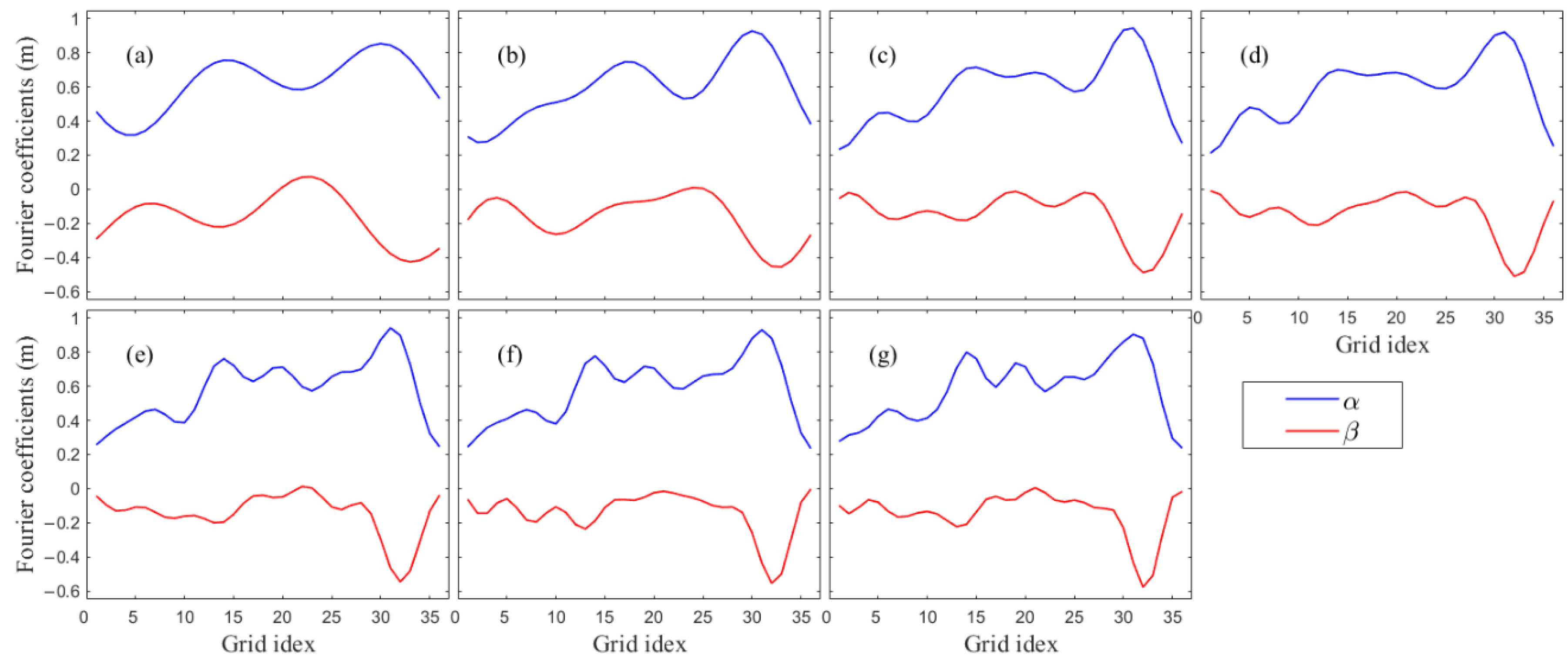
In addition, many physical systems are impaired by some sort of noise. Considering factors including disturbance from the environment and precision of observation instruments, errors are inevitable in actual observations. In the simulation process, there will be approximation and truncation in the model as well. Therefore, TEs 5–8 are conducted to investigate the performance of different methods in the presence of errors. The Gaussian white noise is selected as the error and added into the time series of water elevations, and then OBCs are inverted by adjoint assimilation. Prescribed FCs are constructed from the characteristics of OBCs obtained by inversion in previous studies. The data with noise are generated as follows: the forward model is run with prescribed FCs α and β to obtain “observations”, and then Gaussian white noise is added to the “observations”. Noise–signal power ratio (NSPR) is used as a measure of added white noise value. In TEs 5–8, Gaussian white noise with NSPR of 5%, 10%, 15% and 20% is added to the “observations”, respectively, and FCs α and β are inverted. The inversion process terminates when the number of iteration steps reaches 200. In TEs 5–8, for CI and SI schemes, seven independent points are selected uniformly, and the MTP in TPF scheme is set to 3. The given and inverted FCs are displayed in
Figure 5.
To quantitatively evaluate the results simulated with different methods, the root-mean-square (RMS) error between the simulated water elevations and the observations are calculated according to the following formulation [
6,
25,
48]:
where
and
are the observed tidal amplitudes and phases of the
tidal constituent at the
ith observation points,
and
are the corresponding simulated values and
D is the number of observation points. Smaller RMS error means better consistency between simulated results and the observations.
3.3. Results and Discussion of TEs
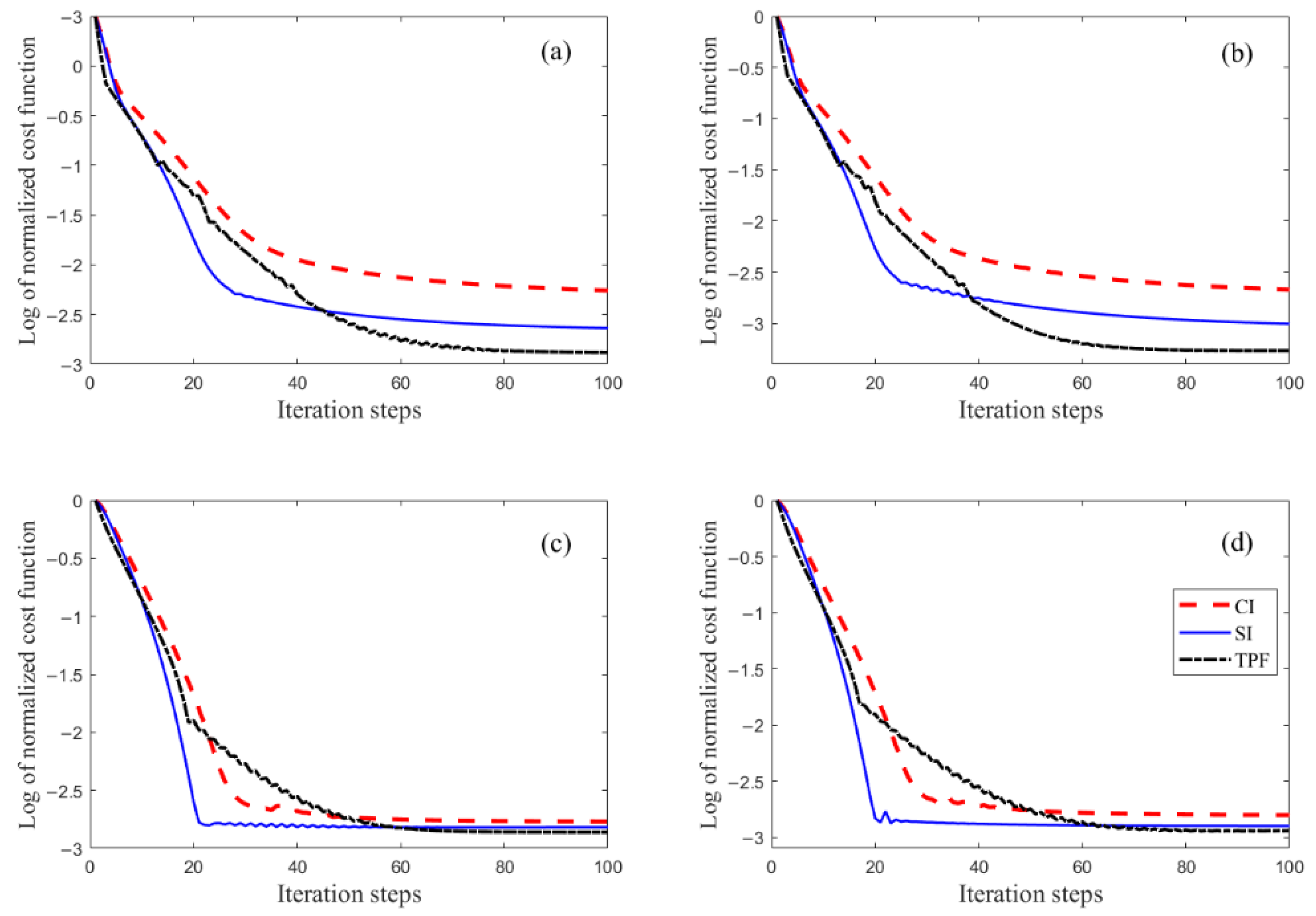
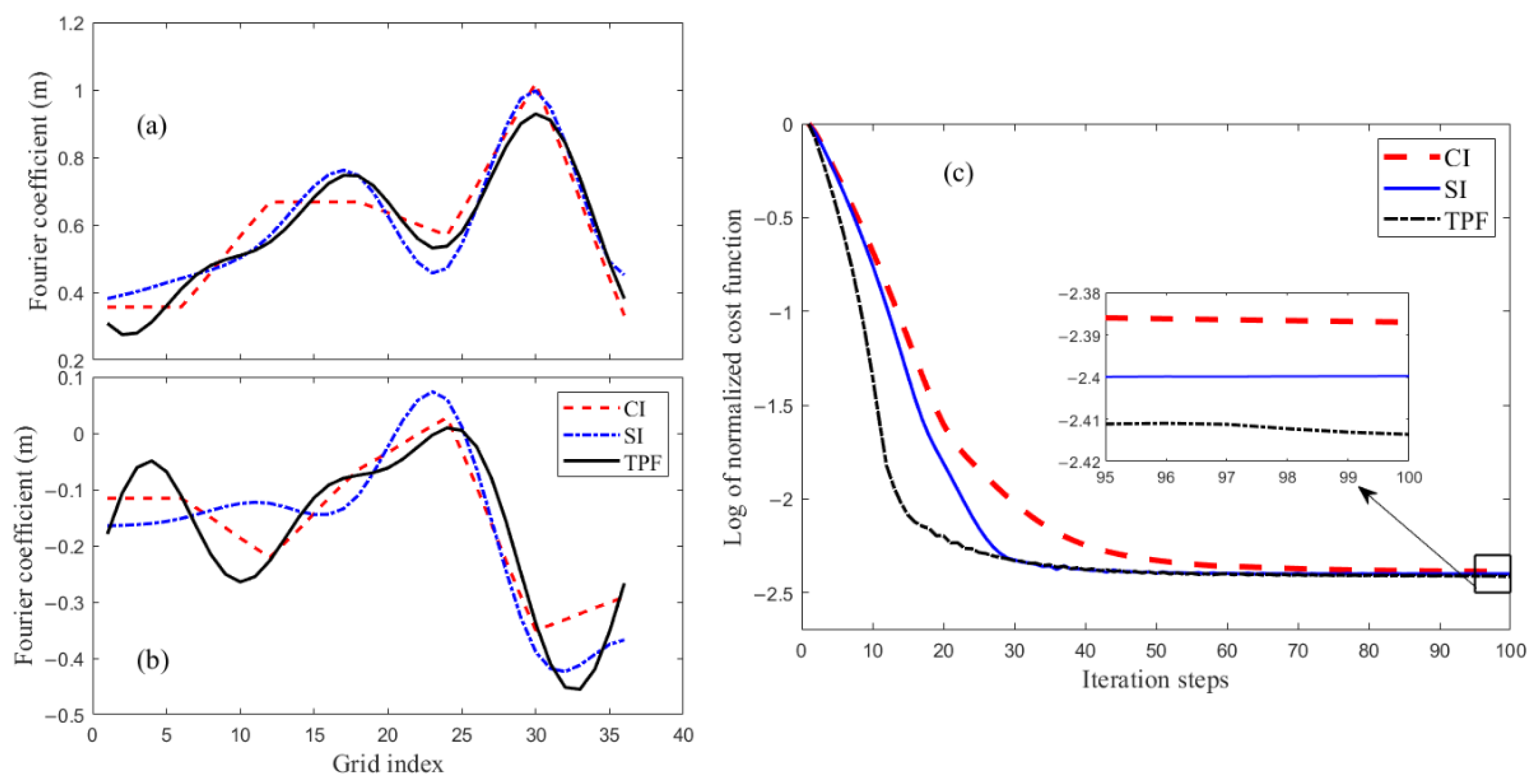
The cost function describes the difference between the simulations and the observations, and its variation with the iteration steps shows the efficiency and stability of the inversion method. The decline in the cost function is described here by the normalized cost function (the ratio of the cost function to its initial value) in log form, which reduces significantly and stabilizes as the iteration step size increases (
Figure 6). It should be noted that, under the influence of normalization, the normalized cost functions only show the decreasing trend and the extent of decrease, while the specific values that the differences can reduce to are reflected by the RMS errors. Correlation coefficients between the prescribed and inverted FCs and RMS errors are calculated as quantitative indicators of the effect of different methods (
Table 1).
The prescribed FCs are successfully inverted by IPs schemes and TPF scheme (
Figure 4); however, the inverted results obtained by TPF and SI scheme are smoother compared with CI scheme. The cost functions decrease to about 10
−3 of their initial values; the cost function of SI scheme descends fastest, while the cost function of TPF scheme can be decreased to a lower level (
Figure 6). Quantitatively, the RMS errors of TEs 1–2 are larger than those of TEs 3–4, and the RMS errors of TPF scheme are the lowest in different TEs, which are 0.17 cm, 0.17 cm, 0.11 cm and 0.09 cm, respectively (
Table 1). The correlation coefficients of inverted and prescribed FCs in TEs 1–4 are all above 0.988. Although a lower RMS error does not guarantee a greater correlation coefficient, the correlation coefficients of TPF scheme in TEs 1–4 maintain at a large level (greater than 0.999). The inverted results and quantitative indicators of TEs 1–4 show that, in the ideal case, the TPF scheme has better performance compared with the IPs scheme in tidal OBCs estimation.
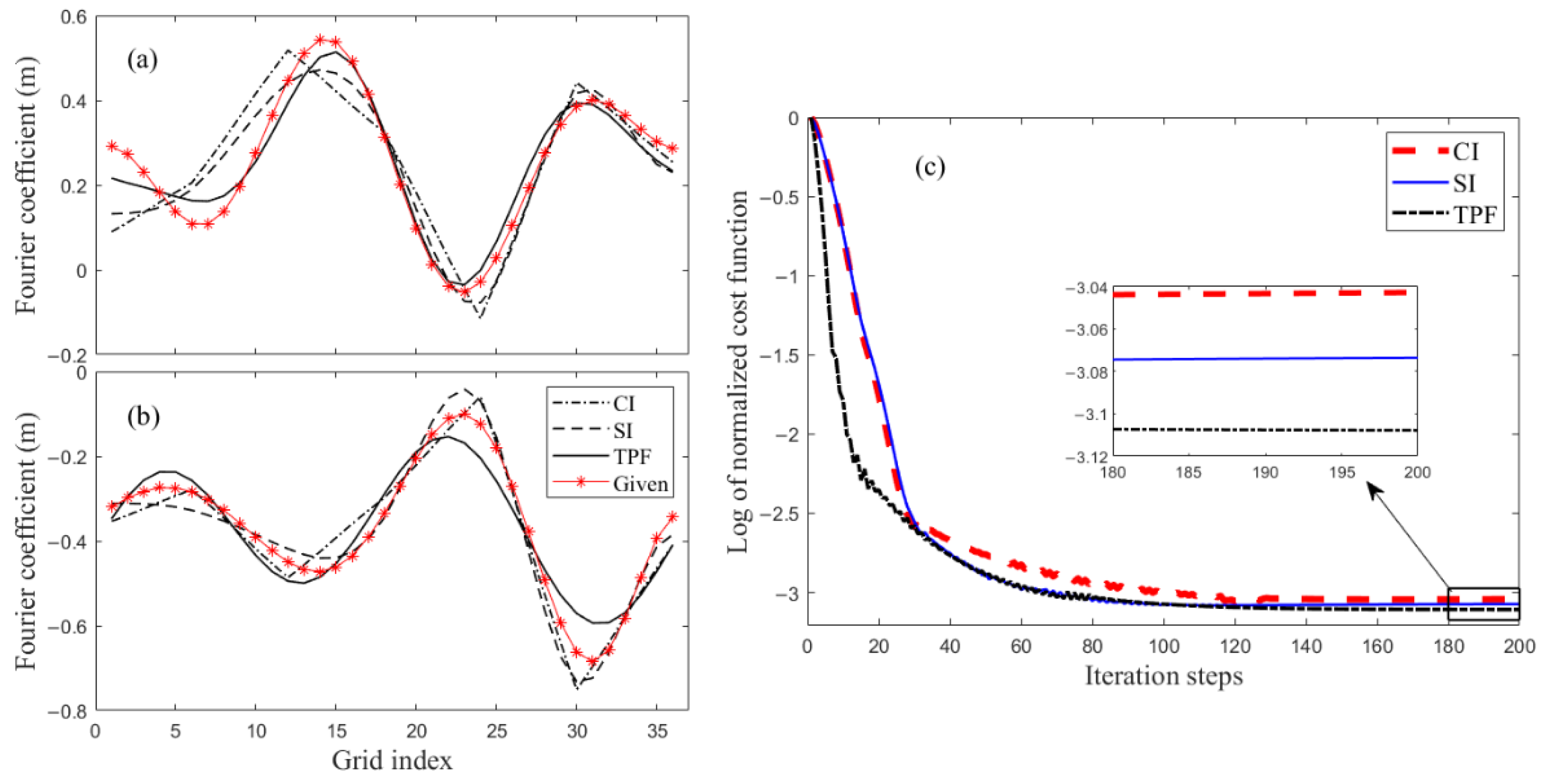
The FCs in TEs 5–8 are also inverted successfully (
Figure 5), and the results of TPF scheme are more consistent with the prescribed FCs. A control experiment without adding white noise is conducted, and the inverted FCs and normalized cost functions are shown in
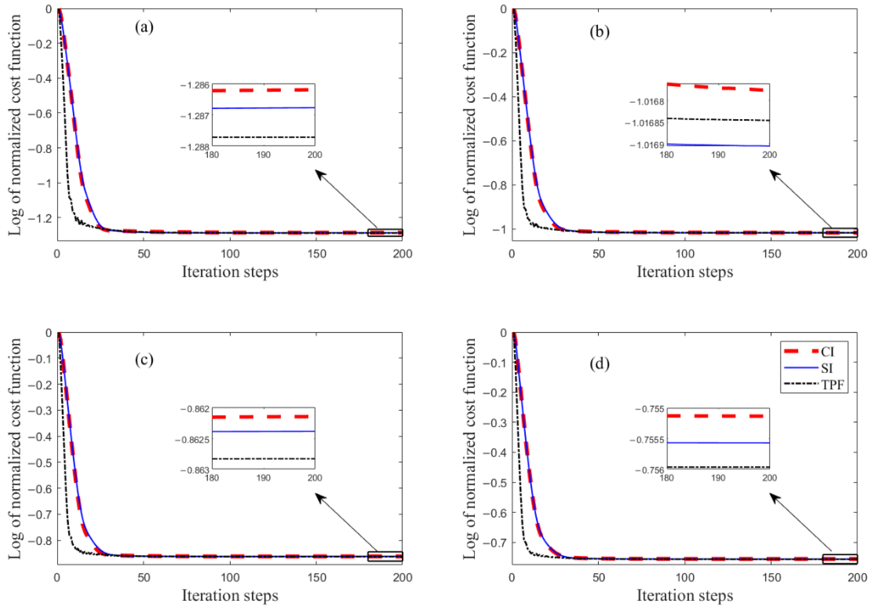
Figure 7. The descent process of cost functions in different experiments (
Figure 8) shows that, with the increase in NSPR, the extent of decrease in cost functions becomes smaller. In contrast to the previous situation, when there exist observation errors, the cost function of the TPF scheme descends faster compared to that of the IPs scheme. The normalized cost function of TPF scheme is the lowest, except in TE-7 (
Figure 8b); however, TE-7 is the experiment with the least difference in normalized cost function by different methods (about 10
−4 orders of magnitude, while other TEs are about 10
−3).
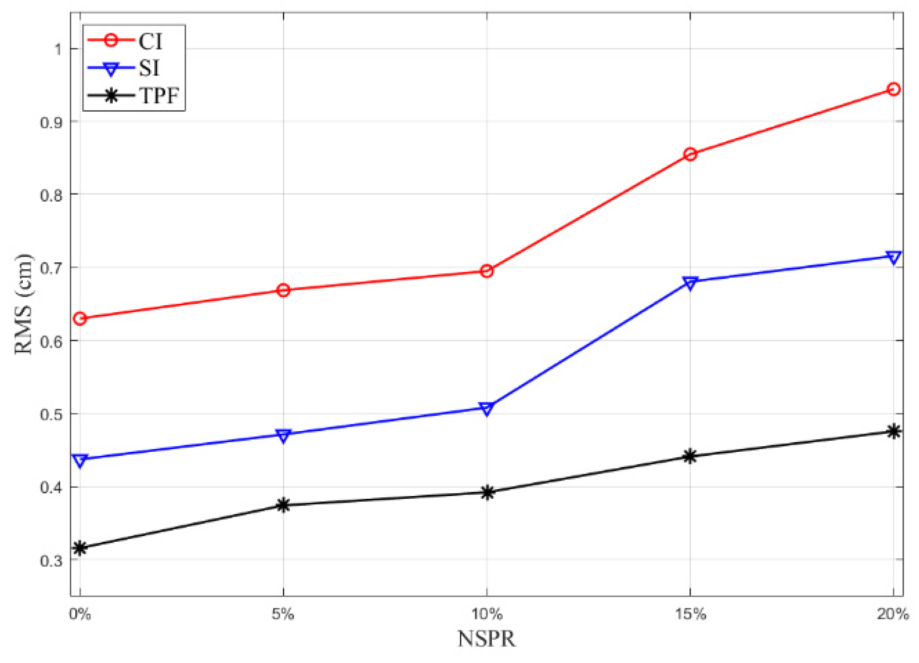
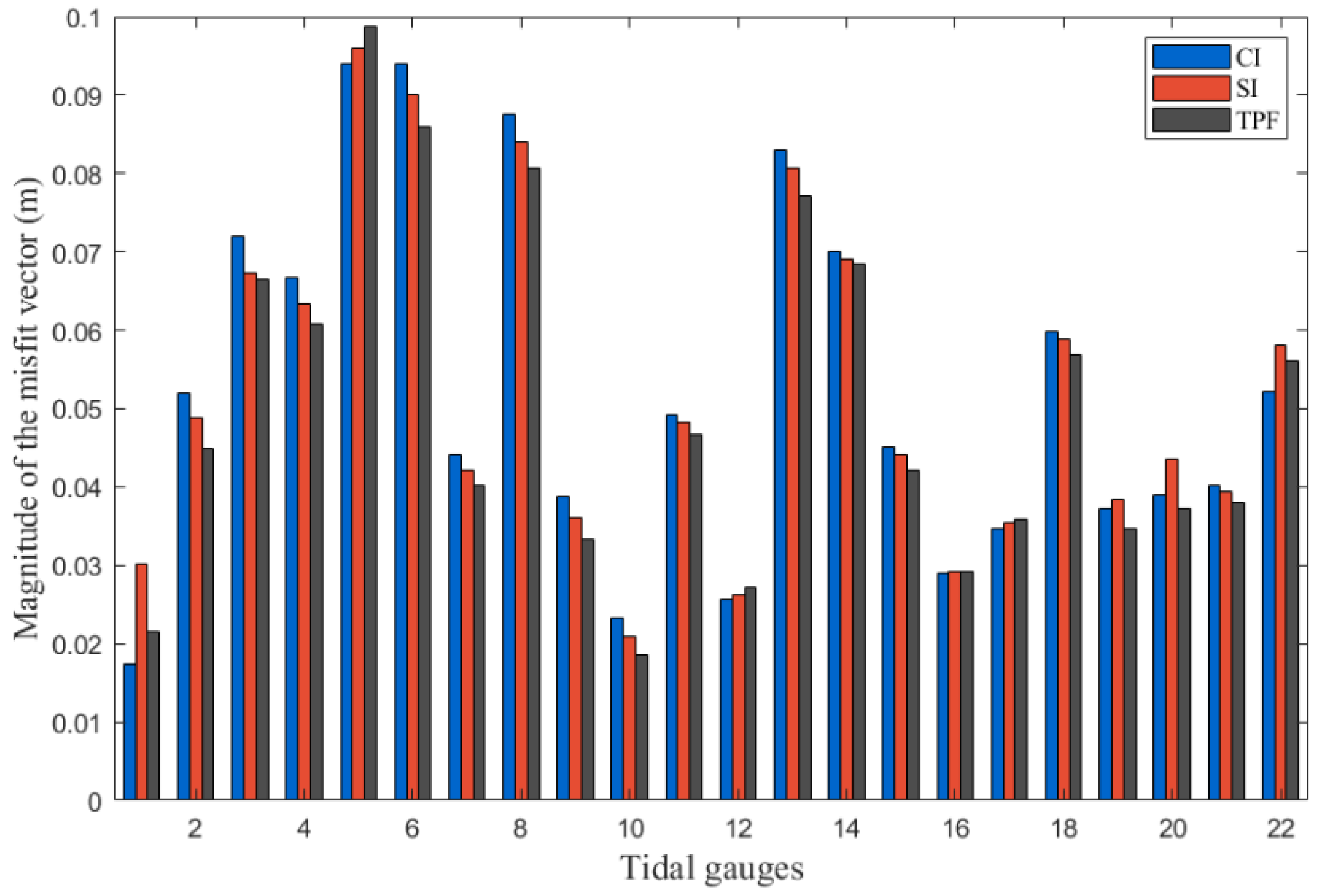
It can be obtained from
Table 2 that, as the NSPR increases, the RMS error also increases, which is shown visually in
Figure 9. By comparison, with the same NSPR used, the RMS error of TPF scheme is the smallest, only 4.8 cm at 20% NSPR, which is better than most results of IPs scheme. The correlation coefficients of β obtained by IPs scheme are slightly higher than those of α, while those of FCs obtained by TPF scheme are closer. The correlation between FCs inverted by TPF scheme and prescribed is better, with all of the coefficients >0.95, which is the best among all approaches. Similar to the results of TEs 1–4, the correlation coefficients are not monotonously decreased with the RMS error. With the increase in NSPR, the correlation coefficients generally show a decreasing trend. The addition of Gaussian white noise does have a negative effect on the inversion. For both IPs scheme and TPF scheme, the higher noise power is, the worse inversion results will be. Compared with CI and SI scheme, TPF scheme is obviously less affected (
Figure 9), indicating its better stability.
In the TEs, OBCs are estimated and water elevations are simulated by assimilating “observations” using different approaches. According to the results of TEs, the FCs inverted by TPF scheme are smoother and closer to the given distribution compared with IPs scheme (
Figure 3 and
Figure 4). In TEs 1–4, quantitative indicators also show that the TPF scheme performs better, the RMS errors of simulation are smaller and correlation coefficients between inverted and given are larger (
Table 1 and
Table 2). In TEs 5–8, white noise of different NSPR is added, and the estimation and simulations of the TPF scheme are less affected by errors, which reflects its better stability. However, the effectiveness of the TPF scheme is affected, as the error in the observed data increases, which means that the scheme is still dependent on the accuracy of the observed data.
5. Conclusions
In this paper, TPF is developed to improve a 2D tidal model and the OBCs of M2 tide are estimated via assimilating altimeter data. The FCs of OBCs are expressed in the form of a discrete Fourier series and the coefficients of trigonometric polynomials are taken as control parameters. The adjoint method is applied to correct the coefficients of trigonometric polynomials to optimize the OBCs.
The M2 constituent is simulated by applying prescribed OBCs, the simulation results on altimeter tracks are selected as “observations” and a series of TEs are constructed by assimilating the “observations”. Considering the actual and model errors, white noise of different NSPR was added into the “observed value” in some twin experiments. The TPF scheme is calibrated and the OBCs are successfully inverted by TPF scheme in TEs. Compared with the IPs scheme, the OBCs obtained by TPF maintain smoothness and are closer to the prescribed distribution, with smaller RMS errors and better stability. In the BYS simulation domain with 1/6° horizontal resolution, T/P-Jason data are assimilated to estimate the OBCs for the M2 tidal constituent. The tidal gauge data are also included to verify the effectiveness of the simulation. The quantitative indicators show that the TPF scheme has a better performance in this simulation domain while MTP is 3. Tidal data derived from TPXO9, FES2014, EOT20, NAO.99b and OSU12 are taken into consideration, which are used to obtain OBCs in the computation domain to verify the performance of TPF scheme. Moreover, compared to the SI and CI schemes, the simulation results of the TPF scheme agree better with the observed data. The cotidal chart simulated with TPF scheme accurately reflects the characteristics of M2 constituent in the BYS.
In conclusion, the TPF scheme is an effective improvement in the estimation of the OBCs in tidal models. However, its effectiveness in use still depends largely on data quantity and accuracy. Supported by observations, TPF scheme can provide more accurate tidal OBCs for the marginal ocean tidal model. In future research, the TPF method can be combined with the estimation of BFCs, eddy viscosity profiles and other parameters in the tidal model and achieve a more accurate simulation of regional tides.


