Article

Blind Hyperspectral Image Denoising with Degradation Information Learning

School of Software Engineering, Xi’an Jiaotong University, Xi’an 710049, China
*
Author to whom correspondence should be addressed.
Remote Sens. 2023, 15(2), 490; https://doi.org/10.3390/rs15020490
Submission received: 27 October 2022 / Revised: 21 December 2022 / Accepted: 23 December 2022 / Published: 13 January 2023
(This article belongs to the Section AI Remote Sensing)

Abstract

:
Although existing hyperspectral image (HSI) denoising methods have exhibited promising performance in synthetic noise removal, they are seriously restricted in real-world scenarios with complicated noises. The major reason is that model-based methods largely rely on the noise type assumption and parameter setting, and learning-based methods perform poorly in generalizability due to the scarcity of real-world clean–noisy data pairs. To overcome this long-standing challenge, we propose a novel denoising method with degradation information learning (termed DIBD), which attempts to approximate the joint distribution of the clean–noisy HSI pairs in a Bayesian framework. Specifically, our framework learns the mappings of noisy-to-clean and clean-to-noisy in a priority dual regression scheme. We develop more comprehensive auxiliary information to simplify the joint distribution approximation process instead of only estimating noise intensity. Our method can leverage both labeled synthetic and unlabeled real data for learning. Extensive experiments show that the proposed DIBD achieves state-of-the-art performance on synthetic datasets and has better generalization to real-world HSIs. The source code will be available to the public.

1. Introduction

As one of the most important topics in remote sensing research, hyperspectral image (HSI) has been extensively applied to various fields, such as environmental geology, vegetation ecology, atmospheric science, oceanography, agriculture, and more [1,2,3,4,5]. However, due to various complicated and unknown noises encountered in imaging and transmission, the quality of HSIs can be severely reduced, directly deteriorating the performance of subsequent HSI applications. Therefore, it is a crucial pre-step to restore the underlying clean HSIs from noisy observations.
HSI denoising is a typical ill-posed problem since infinite mappings exist from a noisy HSI to its clean counterpart in the solution space. A great deal of HSI denoising methods has been proposed in recent years. In general, existing methods can be divided into model-based and learning-based approaches. From the Bayesian perspective, most model-based denoising methods follow the maximum a posteriori (MAP) estimation framework, which relies on the assumption of a specific noise model [6,7,8,9], or empirical HSI priors [10,11,12,13,14] such as low-rank tensors, self-similarity, and so on. These model-based methods have superior performance on pre-setting synthetic HSI datasets with known noise types and parameter settings, such as additive white Gaussian noise (AWGN). However, in real-world imaging and transmission systems, HSI noises come from various factors, such as photon effects, atmospheric absorption, calibration error, etc. [15]. These make real noises largely deviate from the characteristics of parametric noise models like AWGN. Therefore, handling real HSI noises is difficult for model-based methods. Moreover, the iterative optimization procedures in such methods are time-consuming, as shown in Figure 1. Manual parameter adjustment also seriously limits their applications in the real world.
Different from model-based methods, the learning-based methods achieve blind denoising by learning the noisy-to-clean translation through deep neural networks. Thanks to the strong function fitting ability of deep models, learning-based HSI denoising methods have been advanced quickly. To achieve satisfactory performance, these deep models are usually trained on a large amount of noisy-clean HSI pairs in a fully-supervised way. Learning-based methods can be further divided into the single-stage and two-stage frameworks, depending on whether there exist a noise intensity estimation stage. Due to the ill-posed nature, it is difficult to learn the optimal mapping from the noisy to clean without using any prior knowledge for single-stage methods [16,17,18,19,20]. Two-stage methods [21,22,23,24] attempt to estimate the noise intensity as auxiliary information to assist the denoising problem. The real HSI contains more complex noise than Gaussian noise, so guiding the denoiser with the noise intensity prior is inadequate for real-world HSI denoising. Moreover, these fully supervised methods still generalize poorly to real-world noisy HSIs, owing to the scarcity of labeled real-world datasets.
In this paper, we propose a novel Bayesian framework with degradation information learning to tackle the blind HSI denoising problem. Our method (termed DIBD) employs a priority dual-regression scheme that can be trained on mixed data, i.e., the synthetic clean–noisy pairs and unlabeled real-world noisy data. The motivations and main ideas of this work can be summarized in two points below.
On the one hand, learning the joint probability distribution p ( x , y ) could model the full information between the noisy and clean images theoretically [25,26], which is superior than only inferring the posterior distribution p ( x | y ) . However, these generative methods [25,26,27,28] cannot be directly transferred to real-world HSI denoising task, owing to the fact that approximation of true joint probability distribution p ( x , y ) relies on the unpaired real-world clean HSIs which are hard to collect, and most of them are trained with the unstable adversarial training manner. Therefore, the crux is how to stably approximate p ( x , y ) only with the unlabeled noisy HSI in real-world scenario. Inspired by the idea of dual learning [29], we attempt to approximate the joint probability distribution p ( x , y ) in a Bayesian framework from two opposite directions, i.e., the primary denoising path p ( x | y ) p ( y ) and the dual degenerating path p ( y | x ) p ( x ) . Such dual-regression scheme can be seen as imposing spatial-spectral consistency constraints on these two paths. In practice, we design a Denoiser and a Degenerator to tackle these two paths, respectively. The denoiser focuses on recovering the latent clean HSI, and the degenerator aims to restore the original noisy observation from the denoiser’s output. Through the constraint of the degenerator, the better mapping from noisy to clean can be learned by the denoiser. It should be noted that the original dual learning scheme trains the primary and dual paths simultaneously would disregard the priority between the primary and dual tasks [30,31,32,33], failing to approximate the joint distribution well. Obviously, the initial output of the primary path x ^ largely deviates from p ( x ) , leading to a negative effect on the dual degenerating path p ( y | x ) p ( x ) . To address this problem, we propose a simple priority dual regression scheme to better estimate p ( x , y ) . Instead of training the two paths impartially, the denoiser is learned with priority to avoid producing a trivial noisy input to the dual degenerating path.
On the other hand, although the noise intensity (denoted by σ ) has been widely utilized as auxiliary information for AWGN removal [21], the captured real-world HSIs contain more complicated noises, such as multiplicative and impulse noises. Besides noise intensity estimation, in this work, we attempt to extract implicit degradation information (DGInfo, g ) of noisy HSI encoded by a DGExtractor in a latent space. The DGInfo contains both noise and spatial-spectral information in HSIs that can adapt to more complicated real-world situations, greatly improving the generalizability. Then, we concatenate σ and g as the joint auxiliary information (JAInfo, u ) to guide both primary and dual tasks. As JAInfo bridges the gap between noisy and clean HSI domains, our approach can approximate the joint distribution p ( x , y ) better than previous single-stage dual learning methods [33] that ignore degradation information modeling.
The contributions of this work can be summarized from the following three aspects:
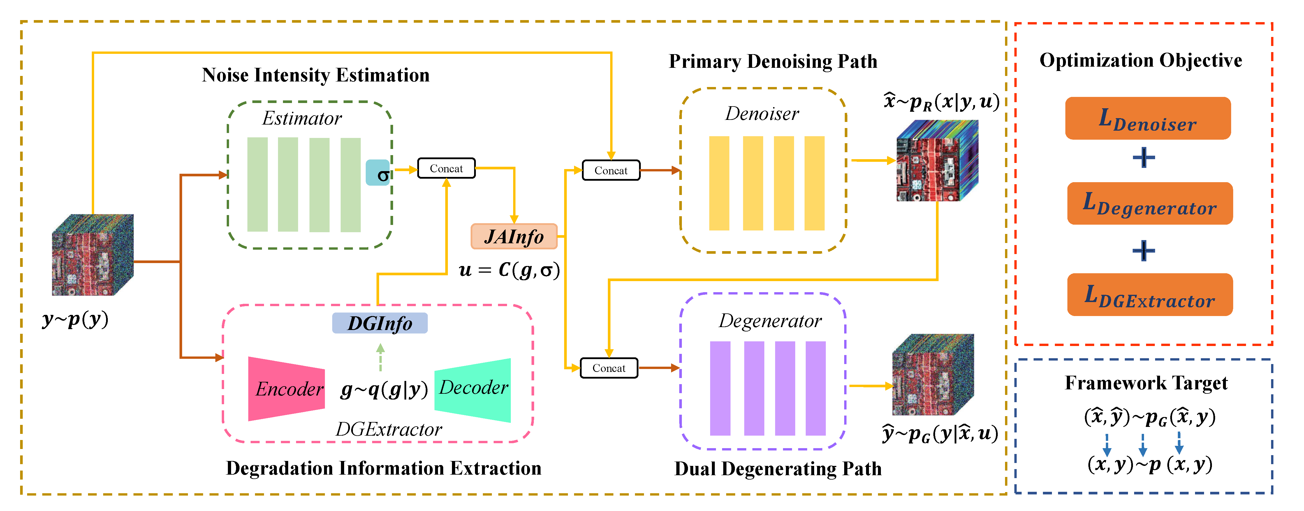
  • We propose a unified Bayesian framework with degradation information learning for HSI denoising. A priority dual regression scheme is built to approximates the joint probability distribution p ( x , y ) .
  • Our method leverages explicit noise intensity and implicit degradation information as joint auxiliary information, which is both beneficial to the primary denoising and dual degenerating tasks.
  • The proposed method can be trained using the synthetic clean–noisy data pairs and the unlabeled HSIs with real noises. Extensive experiments demonstrate that our method achieves state-of-the-art performance both in HSI quality indexes and classification accuracy of real-world HSIs.

2. Related Work

2.1. HSI Denoising

The noise model can be broadly divided into two categories according to different statistical structures, i.e., additive white Gaussian noise (AWGN) and realistic complex noises (e.g., non-i.i.d. Gaussian and sparse noise like stripe, deadline, and impulse). Different from natural image denoising [34,35,36,37,38], which focuses on the information of spatial dimension, various well-designed model-based and learning-based methods have been proposed to remove these noises in HSI over the last decades. These methods attempt to utilize the specific spatial-spectral characteristics in HSIs, and can be interpreted as inferring the posterior distribution p ( x | y ) from the Bayesian perspective.

2.1.1. Model-Based Methods

For AWGN removal, model-based methods employ domain prior knowledge of the HSI, such as global correlation along the spectrum and non-local self-similarity across space. For example, in [39], block matching 4-D (BM4D) based on spatial-spectral non-local mean is designed to remove Gaussian noise. By considering the spatial non-local similarity and local spectral correlation simultaneously, Ref. [40] has had success in Gaussian noise removal. The intrinsic tensor sparsity regularization (ITS) is designed to efficiently explore the underlying characteristics of HSI [6]. In [7], a Hyper-Laplacian regularized unidirectional low-rank tensor recovery model is designed to capture the intrinsic structure correlation in HSI. Recently, [8] achieved state-of-the-art denoising performance thanks to model underlying characteristic of the HSI.
However, the distribution of realistic complex noise largely deviates from the AWGN. Thus, several works have been proposed by modeling the real noise with more complicated features. For example, a low-rank matrix recovery (LRMR) based method is proposed to handle the sparse noise [41]. In [42], a low-rank matrix factorization-based method with the constraint of total-variation and L1 -norm (LRTV) is proposed. Chen et al. [10] propose a robust method by modeling the noise with a non-i.i.d. the mixture of Gaussian (NMoG) noise assumption. By distinguishing the intrinsic structures of clean HSI and complex noise, Wang et al. [11] propose a tensor-based HSI noise removal algorithm. Recently, He et al. [12] designed a low-rank matrix recovery-based method with the constraint of global spatial-spectral total variation.

2.1.2. Learning-Based Methods

Different from model-based methods, learning-based methods can effectively capture the intrinsic features of HSIs, which can blind remove various noises in HSI and achieve fast inference. Specifically, based on the 2D deep learning, Chang et al. [43] first introduce the CNN into the HSI denoising task. Simultaneously considering spatial-spectral information, ref. [16] presents great HSI denoising performance. Cao et al. [18] propose a deep spatial-spectral global reasoning network for HSI noise removal. Due to a large number of spectral dimensions, 3D deep learning can extract spatial-spectral features simultaneously. For example, refs. [17,44,45] constructed a U-Sharp network with different forms of 3D convolution to remove noise in HSIs. Refs. [21,23] fully exploit the rich spectral information in HSI and utilize the presetting noise intensity map as prior knowledge to guide network denoising. A denoising network with a noise intensity estimator is proposed to remove inconsistent and mixed noises in HSIs adaptively [22,24]. The learning-based methods achieve excellent performance in various noise removal tasks, but there is much room for improvement.

2.2. Unpaired Degradation Modeling and Unlabeled Degradation Modeling

Real-world noise removal has been a challenging task due to the scarcity of paired clean–noisy datasets for real-world scenarios. To alleviate these issues, several methods [25,27,28] employ the generative adversarial network (GAN) [46] to learn the degradation of unpaired real-world images. For example, DANet [25] approximates the joint distribution p ( x , y ) from two opposite tasks (i.e., image denoising and noise generation) in a dual adversarial manner. However, these GAN-based methods cannot be directly transferred to real-world HSI denoising tasks, mainly in two aspects. First, to approximate the true joint probability distribution p ( x , y ) , these GAN-based methods rely on the unpaired real-world clean images. In contrast, most real-world HSIs are unlabeled and degraded by various complex noises. Second, GAN-based methods with unstable training need elaborate fine-tuning of different parts of adversarial losses, leading to hard in learning a good noise generator. By contrast, our method can be trained using the synthetic clean–noisy data pairs and the unlabeled real-world noisy HSIs with a priority dual regression scheme instead of the adversarial learning.

2.3. Dual Learning vs. Priority Dual Learning

Dual learning is first proposed in [29], which learns two opposite tasks simultaneously in a close-loop framework. In recent years, some works adopt this scheme for high-level tasks [30,31] and low-level tasks [32,33] to improve the performance of whole network. At the same time, all of these methods disregard the priority between the primary and dual tasks, learning the two paths impartially. By contrast, we propose a simple priority dual regression scheme, which learns the denoiser with priority to avoid producing a trivial noisy input to the dual clean-to-noisy path. Moreover, we consider the importance of degradation information for the dual degenerating task and feed the learned degradation information into our priority dual regression scheme.

3. Proposed Method

In real-world scenarios, HSI is usually degraded by various mixed noises. These noises have more complicated statistical distribution and might largely deviate from the AWGN. Therefore, to achieve blind HSI denoising, we developed joint auxiliary information and utilized it to guide the primary and dual network simultaneously. The details of the proposed Bayesian framework are explained as follows.

3.1. Joint Auxiliary Information

As mentioned above, the JAInfo is composed of the explicit noise intensity σ and the implicit DGInfo g of noisy HSI y , where y p ( y ) denotes sampling from training dataset. The noise intensity estimation σ of each band in noisy HSI y can be formulated as
σ ^ q ( σ | y ) ,
where σ ^ can be seen as sampling from the following implicit distribution q ( σ | y ) learned by the estimator.
Different from previous degradation learning-based methods, such as [47], our motivation is that the noisy HSIs can be generated in a procedure involving the DGInfo g , which naturally implies both noise-relevant information and specific spatial-spectral correlation in HSIs, can be extracted by reconstructing the noisy HSIs with a simple 3D-VAE effectively. Then, we assume the DGInfo g comes from a latent variable, which randomly sampled from latent space to avoid over-fitting problems. Such implicit DGInfo can handle more complicated noise situations. In the DGExtractor that consists of an encoder and decoder, the inference process of g can be expressed as
y q ( g | y ) g p ( y | g ) y rec .
To approximate the posterior p ( g | y ) , q ( g | y ) is introduced and described as q ( g | y ) = N ( μ , ς 2 ) with the encoder. Then the probability distribution log p ( y ) can be reformulated as
log p ( y ) = E g q ( g | y ) [ log p ( y | g ) ] + D K L ( q ( g | y ) p ( g | y ) ) D K L ( q ( g | y ) p ( g ) ) ,
with prior distribution p ( g ) , which can be easily set as an Gaussian distribution N ( 0 , I ) with zero mean and unit covariance. To minimize D KL ( q g | y p g | y ) , the corresponding evidence lower bound (ELBO) L is defined as
E L B O = E g q ( g | y ) [ log p ( y | g ) ] D K L ( q ( g | y ) p ( g ) ) .
Therefore, the implicit DGInfo g can be obtained by maximizing the ELBO. Then, the proposed JAInfo u is defined as the concatenation of noise intensity estimation σ ^ with the implicit DGInfo g
u = Concat ( σ ^ , g ) ,
where u q ( σ , g | y ) . Noticeably, the noise intensity σ is estimated by [48] directly, which is not involved in the training process. Hence, q ( σ , g | y ) = q ( σ | y ) q ( g | y ) .

3.2. Joint Distribution Approximation

The objective of most existing HSI denoising methods can be seen as approximating the conditional distribution p ( x | y ) , which lost a lot of information between x and y . To solve the limitation, our approach attempts to approximate the joint probability distribution p ( x , y ) in two opposite directions through a priority dual regression manner, i.e., primary denoising path p ( x | y ) p ( y ) and dual degenerating path p ( y | x ) p ( x ) . The additional auxiliary information can make the primary and dual network easier to tackle the denoising and degenerating tasks respectively, and the proposed JAInfo u is fed to these two tasks as guidance.
For the primary denoising task, the denoiser takes the combination of noisy HSI y p ( y ) and JAInfo u q ( σ ^ , g | y ) as inputs, and tries to learn an implicit distribution p R ( x | y , u ) as close to the true distribution p ( x | y , u ) as possible, which outputs the noiseless result x ^ . Thus, the simulated joint distribution p R ( x , y ) can be approximated by
σ g p R ( x | y , σ , g ) q ( σ | y ) q ( g | y ) p ( y ) d g d σ .
In such way, the pseudo noisy image pairs ( x ^ , y ) can be sampled from p R ( x , y ) .
For the dual degenerating task, the degenerator restores the original noisy HSI y from the noiseless output x ^ of the denoiser. Then, the degenerator attempts to learn an implicit distribution p G ( y | x ^ , u ) to approximate the true distribution p ( y | x , u ) . Suppose u is only related to y , the simulated joint distribution p G ( x ^ , y ) can be approximated by
u p G ( y | x ^ , u ) q ( x ^ ) q ( u ) d u .
Therefore, we can sample the pseudo noisy image pairs ( x ^ , y ^ ) from p G ( x ^ , y ) .
So far, we have approximated the joint distribution p ( x , y ) in two opposite directions. In addition, under the case of mini-batch size being large enough [49], Equation (6) can be approximated to
p R ( x , y ) p R x | y , u p ( y ) ,
and Equation (7) also can be expressed as
p G ( x ^ , y ) p G y | x ^ , u p ( x ^ ) .
In fact, any clean–noisy HSI pair can be seen as one example sampled from the joint distribution. Therefore, two pseudo clean–noisy HSI pairs ( x ^ , y ) and ( x ^ , y ^ ) are expected to approximate the true clean–noisy HSI pair ( x , y ) . Such a priority dual regression scheme can reduce the solution space effectively. The denoiser and degenerator promote each other mutually, gradually pushing two pseudo joint distributions toward the true joint distribution.

3.3. Optimization Objective

The next fundamental problem is to clear and definite the optimization objective of the proposed method, which consists of several parts, i.e., (NI) Estimator, DGExtrator, Denoiser, and Degenerator, where the (NI) Estimator does not participate in the optimization process. To alleviate over-smoothed results by using mean square error (MSE) loss, we adopt the mean absolute error (MAE) loss as the final loss function. The optimization objectives are explained as follows.

3.3.1. DGExtrator

Instead of directly minimizing the KL divergence between q ( g | y ) and p ( g | y ) , the g can be obtained by maximizing the ELBO. The first term of ELBO is noisy HSI y reconstruction of the decoder. Thus, the MAE loss function is
L D e c o d e r = y y rec 1 ,
where y rec denotes the output of decoder, and the second term of ELBO can be calculated as follows
D K L ( q ( g | y ) p ( g ) ) = D K L N μ , ς 2 | | N ( 0 , 1 ) = 0.5 1 + log ς 2 μ 2 ς 2 .

3.3.2. Denoiser and Degenerator

In order to approximate the joint distribution p ( x , y ) as well as possible, two pseudo clean–noisy HSI pairs ( x ^ , y ) and ( x ^ , y ^ ) are expected to approach the true clean–noisy HSI pair ( x , y ) . Actually, we only need to reduce the gap between ( x ^ , y ^ ) and ( x , y ) due to the proposed priority dual regression scheme, which corresponds to minimize the distance between x and x ^ , y and y ^ . Thus, the loss function of the denoiser can be defined as
L D e n o i s e r = x x ^ 1 ,
where x and x ^ denote the clean HSI and the output of the denoiser, respectively. Similarly, the loss function of the degenerator can be described as below
L D e g e n e r a t o r = y y ^ 1 ,
where y and y ^ denote the original noisy HSI and the output of the degenerator, respectively.

3.3.3. Overall Loss

Up until now, the holistic network optimization objective can be obtained as follows:
L O v e r a l l = L D e n o i s e r + λ L D e g e n e r a t o r + L D G E x t r a c t o r ,
where λ is empirically set to 0.01 for full-supervised training scenarios. L D e n o i s e r is set to 0 for real-world unlabeled data training scenarios.

3.4. Network Architecture

Based the analysis above, the execution process and complete training steps of the whole network is illustrated in Figure 2 and Algorithm 1, respectively. First, the estimator takes the noisy HSI y to produce the estimated noise intensity map σ ^ . At the same time, the encoder generates parameters μ and ς . Through adopting the reparameterization trick, the implicit DGInfo g can be calculated as
g = ϵ ς + μ ,
where ϵ N ( 0 , I ) . Then, the JAInfo u can be obtained by concatenating the σ ^ with g along the channel axis. To feed u to the denoiser and degenerator in a simple way, we also concatenate the input of the denoiser with the JAInfo u along the channel axis, and do the same with the degenerator.
Algorithm 1 The priority dual learning algorithm.
Input: labeled synthetic HSIs ( x s , y s ) , unlabeled real HSIs y r .
Output: Trained model.
1: Initialize Denoiser, Degenerator and DGExtractor.
2: // Train the primary task preferentially.
3: while not convergent do
4:    Sample a batch of synthetic data ( x s , y s ) .
5:    Estimate noise intensity σ with Estimator.
6:    Get implicit degradation information g with DGExtractor.
7:    Feed u = Concat ( σ , g ) to Denoiser and Degenerator.
8:    Update DGExtractor and Denoiser by minimizing
        L D G E x t r a c t o r + L D e n o i s e r .
9: end while
10: // Train the primary and dual tasks jointly.
11: while not convergent do
12:    Sample a batch of synthetic and real data { ( x s , y s ) , y r }.
13:    Estimate noise intensity σ with Estimator.
14:    Get implicit degradation information g with DGExtractor.
15:    Feed u = Concat ( σ , g ) to Denoiser and Degenerator.
16:    if is synthetic data then
17:        Update DGExtractor, Denoiser, and Degenerator by minimizing
            L D G E x t r a c t o r + L D e n o i s e r + λ L D e g e n e r a t o r .
18:    else
19:        Update DGExtractor and Degenerator by minimizing
            L D G E x t r a c t o r + λ L D e g e n e r a t o r .
20:    end if
21: end while
The network structure of each part is further explained as follows. We adopt 3D convolution for each part of our model to better exploit spectral correlation. Specifically, for the denoiser, we design a modified U-Net [50] with embedded residual dense blocks (RDB) [51] to effectively extract the multi-scale spatial-spectral joint features. In Table 1, the depth of RDB in block 3 and 9 are set to 2, and block 5 and 7 are set to 3. For the degenerator, we adopt three convolutional layers with filter number 32 and kernel size 3 × 3 × 3, 3 × 3 × 3, and 1 × 1 × 1 as a degradation block, and the LeakyReLU follows the first convolutional layer. Then, a skip-connection is formed by adding the input to the last layer’s output of the degradation block. Finally, two successive degradation blocks form the degenerator, as shown in Table 2. The DGExtractor consists of an encoder and decoder. The structure of the encoder and decoder are symmetrical as presented in Table 3 and Table 4. The input and output of the encoder have the same channel number. In the encoder, two convolution layers with kernel size 2 × 2 × 1 and stride 2 × 2 × 1 are used to downsample the spatial resolution. Correspondingly, the transpose convolution with kernel size 2 × 2 × 1 and stride 2 × 2 × 1 is adopted to upsample the spatial resolution of the feature map. All the modules’ channel number of the middle feature map is set to 32 except the denoiser.

4. Experiments and Discussions

In this section, we conduct a series of experiments on synthetic and real-world benchmark datasets to evaluate the proposed DIBD comprehensively. The detailed information about these experiments is introduced as follows.

4.1. Experimental Settings

4.1.1. Benchmark Datasets

To train the proposed DIBD, we randomly select 100 images with the size of 1392 × 1300 × 31 from the ICVL hyperspectral dataset [52], which contains 201 images. Then, these selected hyperspectral images are cropped into 1024 × 1024 × 31 as the training samples. Next, several operations are employed to augment the training dataset, including random flipping, rotation, and scaling. Correspondingly, the HSIs are cropped as the cube data with the size of 64 × 64 × 31, and about 53k samples are obtained.
As for the testing set, both synthetic data and real-world data are considered. Except for the 100 training images, the rest images of the ICVL hyperspectral dataset with shape 512 × 512 × 31 and the remote sensing dataset Washington DC with size 200 × 200 × 191 are used for synthetic noise experiments. Moreover, to further evaluate the generalization ability and the robustness of our proposed model, the remote sensing datasets, including Pavia University [53], Indian Pines [54], and Urban [55] are used for real HSI denoising experiments, which are degraded with unknown noise. Among them, Pavia University is acquired by the ROSIS sensor with 103 spectral bands, and we crop the center area with size 220 × 220 × 103. Indian Pines with size 145 × 145 × 220 and Urban with size 307 × 307 × 210 are collected by the AVIRIS sensor and HYDICE hyperspectral system, respectively. Moreover, in the ablation study, the CAVE dataset [56] is also selected to evaluate the generalization ability of different models, where the testing HSI in CAVE is the same shape 512 × 512 × 31 as the ICVL testing data. Notably, due to the characteristics of 3D convolution, the proposed DIBD does not enforce the number of spectral bands, and can freely process HSIs with arbitrary bands.

4.1.2. Comparison Methods

We compare our DIBD with representative model-based and learning-based methods. Specifically, the low-rank matrix recovery methods (LRMR [41], LRTV [42]), 2D learning-based methods (HSIDCNN [16], GRN [18]) and 3D learning-based methods (QRNN3D [17], DPHSIR [23]) are employed in all types of noise removal experiments. In addition, for AWGN removal, the filtering-based method (BM4D [39]), tensor-based methods (TDL [40], ITSReg [6], NG-Meet [8]) are fairly selected. For complex noise removal, the low-rank matrix recovery methods (NMOG [10]) and low-rank tensor methods (LRTDTV [11], LLRGTV [12]) are fairly adopted.

4.1.3. Evaluation Indexes

For synthetic noise experiments, the peak signal-to-noise ratio (PSNR), structure similarity (SSIM) [57], and spectral angle mapper (SAM) [58] are employed to evaluate the result of synthetic experiments quantitatively. For real-world experiments, the overall accuracy (OA) and kappa coefficient are used as objective indexes for assessing the quality of denoised real HSIs.

4.1.4. Synthetic Noise Setting

To evaluate the denoising performance under the AWGN, the different noise intensities σ are applied, i.e., 30, 50, 70 and blind σ [30, 70]. For blind noise removal, model-based methods and DPHSIR require pre-provided noise intensity as the prior, and the blind noise is estimated by [48]. To simulate the various noises which usually corrupt real-world HSIs during the acquisition process, we design five types of complex noise cases which are added to the clean HSIs, and the detail of these additive complex noises are defined as follows:
  • Case 1: Non-i.i.d. Gaussian Noise. The zero-mean Gaussian noise with different intensities, randomly chosen from 10 to 70, is added to each band of the HSI data. Furthermore, such noise is adopted for the other four cases similarly.
  • Case 2: Non-i.i.d. Gaussian + Stripe noise. Non-i.i.d. Gaussian Noise is added as mentioned in case 1. Moreover, the stripes on the column are contaminated in one-third of the bands, randomly selected, and the range of stripes proportion of each chosen band is set to 5% to 15% randomly.
  • Case 3: Non-i.i.d. Gaussian + Deadline noise. All bands are contaminated by non-i.i.d. Gaussian noise as in case 1. Furthermore, the deadline noise is added with the same strategy of stripes noise in case 2.
  • Case 4: Non-i.i.d. Gaussian + Impulse noise. In addition to the non-i.i.d. Gaussian noise in case 1, one-third of bands are randomly selected to add impulse noise with different intensities. The proportion of impulse ranges from 10% to 70%.
  • Case 5: Mixed Noise. The non-i.i.d. Gaussian noise in case 1, the stripe noise in case 2, the deadline noise in case 3, and the impulse noise in case 4 are mixed to contaminate the HSIs with the same strategy of each corresponding case.

4.1.5. Training Strategy

The training process is divided into three stages to improve the model’s robustness and the training efficiency. The corresponding real noisy data is added to mixed-data training for real noise removal. The Adam optimization algorithm [59] is adopted to train the proposed network. First, the network is trained at non-blind zero mean additive white Gaussian noises with noise level σ = 50. If adopting the priority dual regression scheme, the degenerator is added to the training process after finishing the first stage. Then, the network is trained at blind AWGN with σ selected from 30 to 70 uniformly. Finally, the whole network is trained with complex noises randomly selected from case 2 to case 4. Moreover, the learning rate for all three stages is initialized to 2 × 10 4 and decayed when the accuracy of the network does not improve anymore. In the first stage, the number of training epoch is set as 30 with batch size = 16. In the second stage, the number of training epoch is set as 20 with batch size = 64. In the final stage, the number of training epoch is 50 with batch size = 64. In order to compare our approach fairly, we manually adjust the parameters of model-based methods to achieve optimal performance and retrain data-driven-based methods with the same training data and strategy. All the experiments are performed on a server with Intel(R) Xeon(R) CPU E5-2687W v4 @ 3.00 GHz, NVIDIA TITAN XP GPU.

4.2. Experimental Results and Analysis

4.2.1. AWGN Removal

We employ the second stage’s trained model to evaluate the denoising performance in all AWGN cases. The quantitative comparison of denoising results on 50 testing HSIs of the ICVL dataset are represented in Table 5. Compared with all competing methods except DPHSIR in σ = 30 and 50, the proposed DIBD achieves the better results for each quality index in all AWGN cases. Noticeably, DPHSIR removes the AWGN in the non-blind way where the addition noise intensity is expected to provide manually, which makes it hard to apply in real-world scenarios. The visual effects of different denoising methods under noise intensity σ = 50 are presented in Figure 3. Model-based methods, such as BM4D, LRTV, and TDL, produce blurring artifacts in some areas. Other methods can remove Gaussian noise well, but some content details are still lost. In contrast, the proposed DIBD can effectively remove the Gaussian noise while finely preserving the details of HSIs.

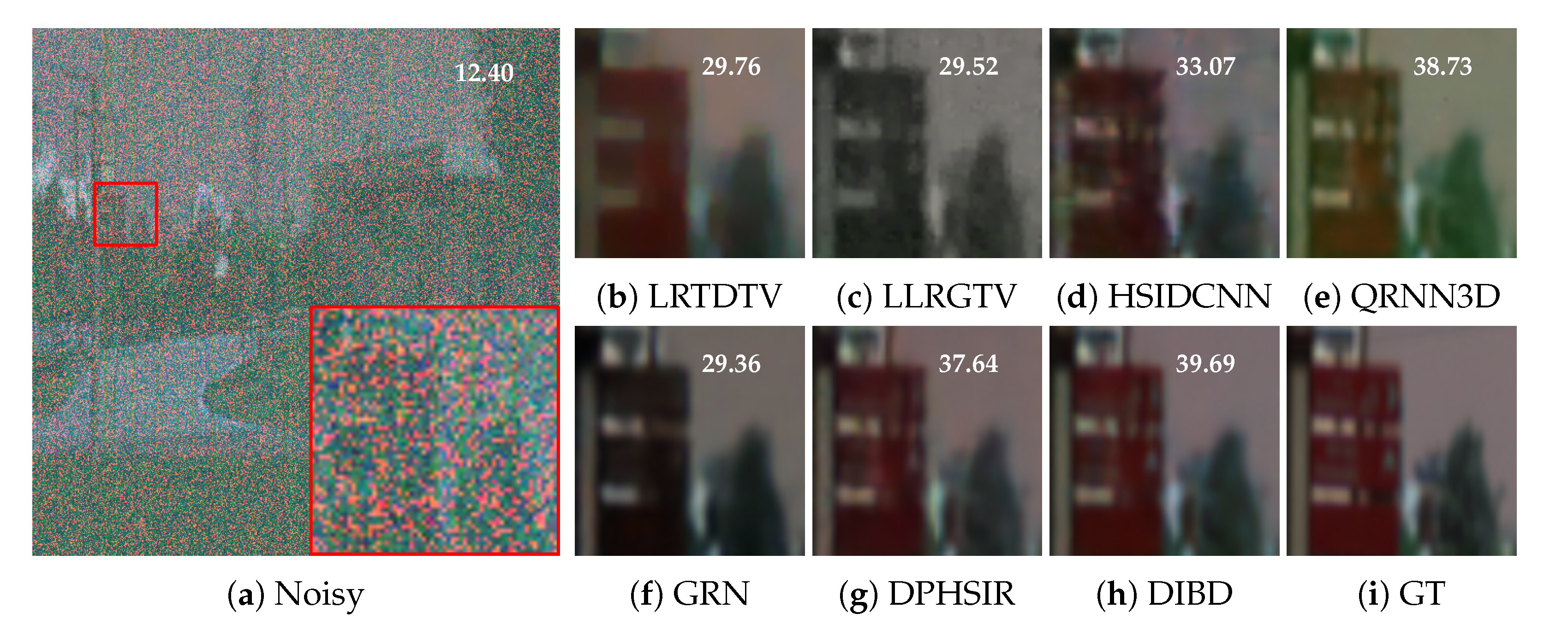
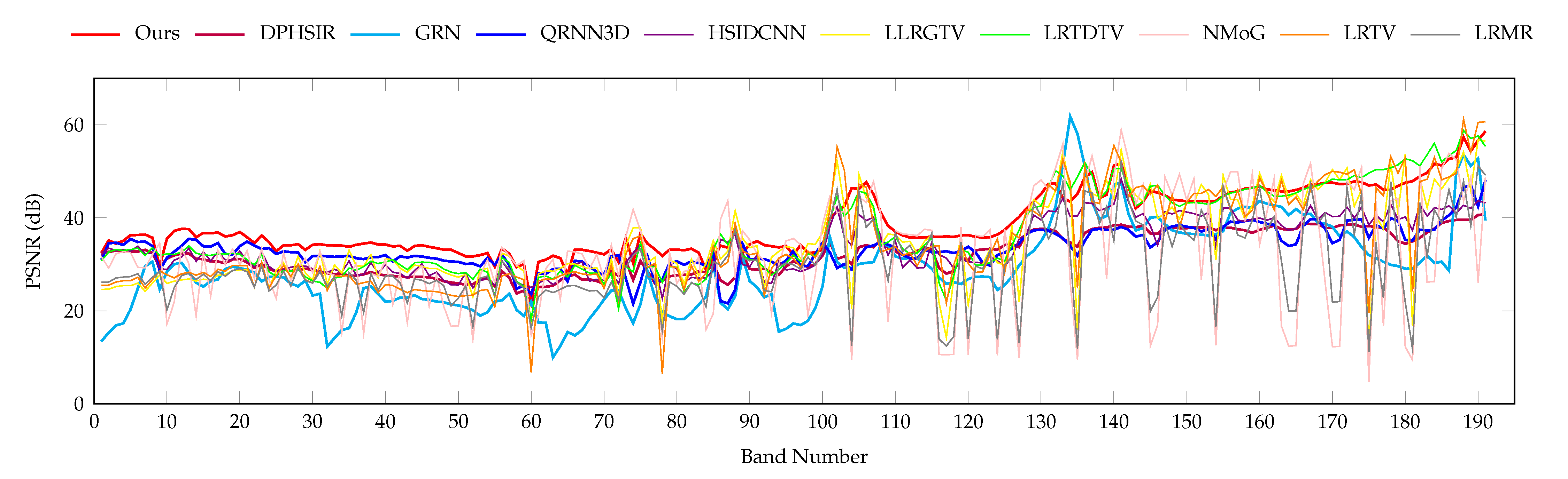
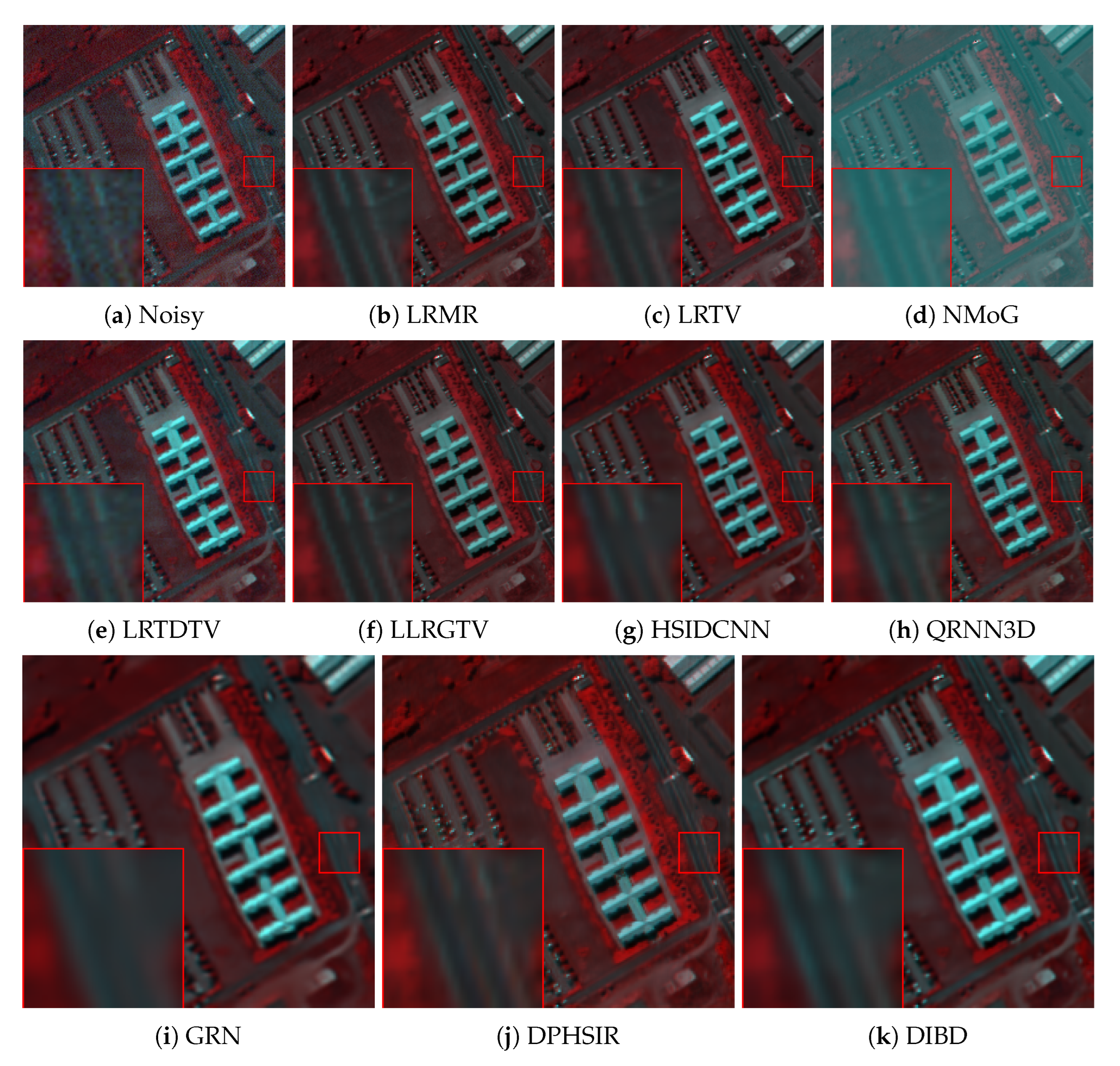
4.2.2. Complex Noise Removal

For complex noise removal, the third stage’s trained model is adopted to evaluate the denoising performance in five complex noise cases. The denoising quantitative results on the ICVL dataset are presented in Table 6. Most methods cannot perform well in case 5, which contains mixed complex noise. Our proposed DIBD’s performance rises over the second best method, QRNN3D, boosting from 41.16 dB to 42.25 dB. The visual effects are shown in Figure 4 and Figure 5. To further prove our DIBD generalization ability and robustness, we conduct complex noise removal experiments on remote sensing images. Since our model can be flexibly applied to HSI with various spectral dimensions, we still use the third stage’s trained model to evaluate the denoising performance directly. The quantitative results and visual effects of Washington DC are shown in Figure 6. The PSNR value across the spectrum is presented in Figure 7. Compared with other advanced methods, our proposed DIBD can better filter out complex noise and maintain the fine-grained structure of HSIs.

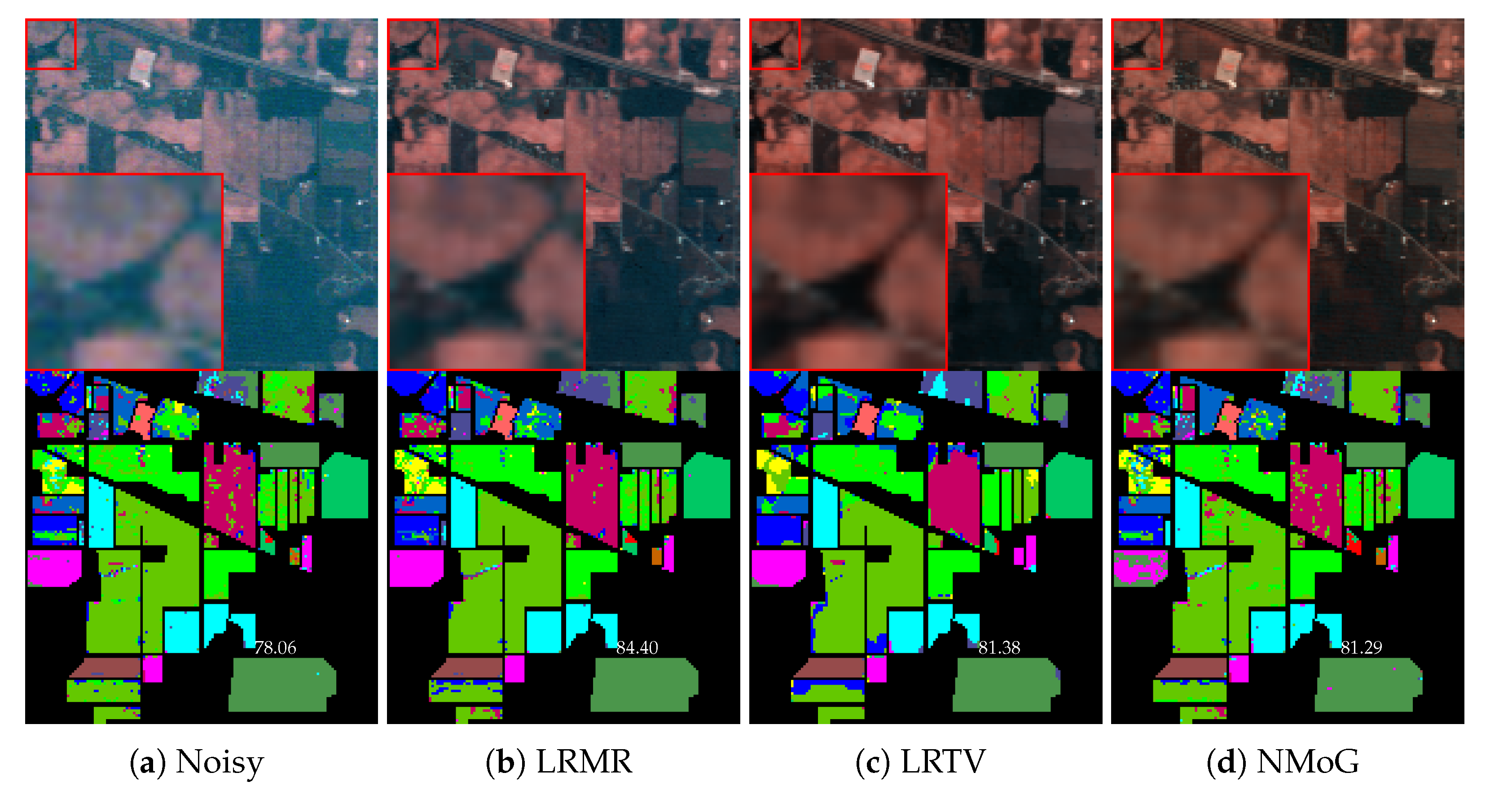
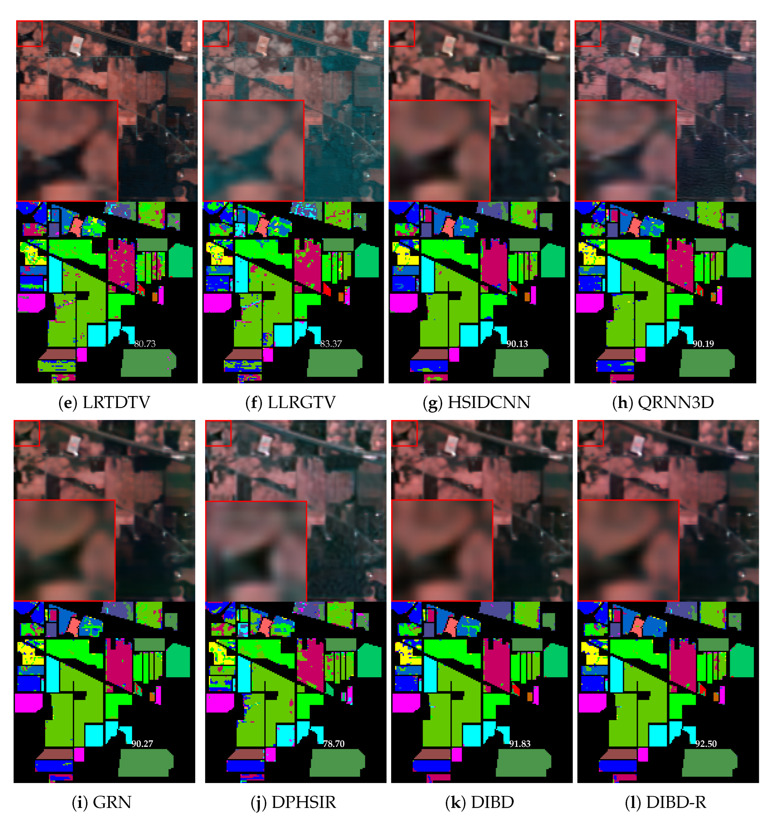
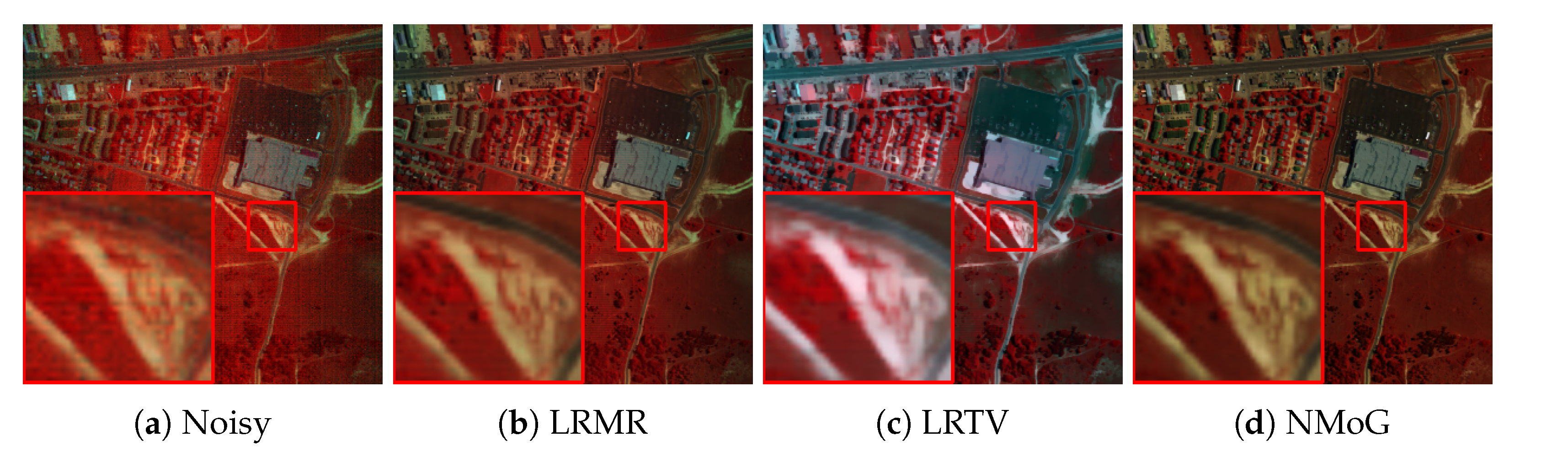
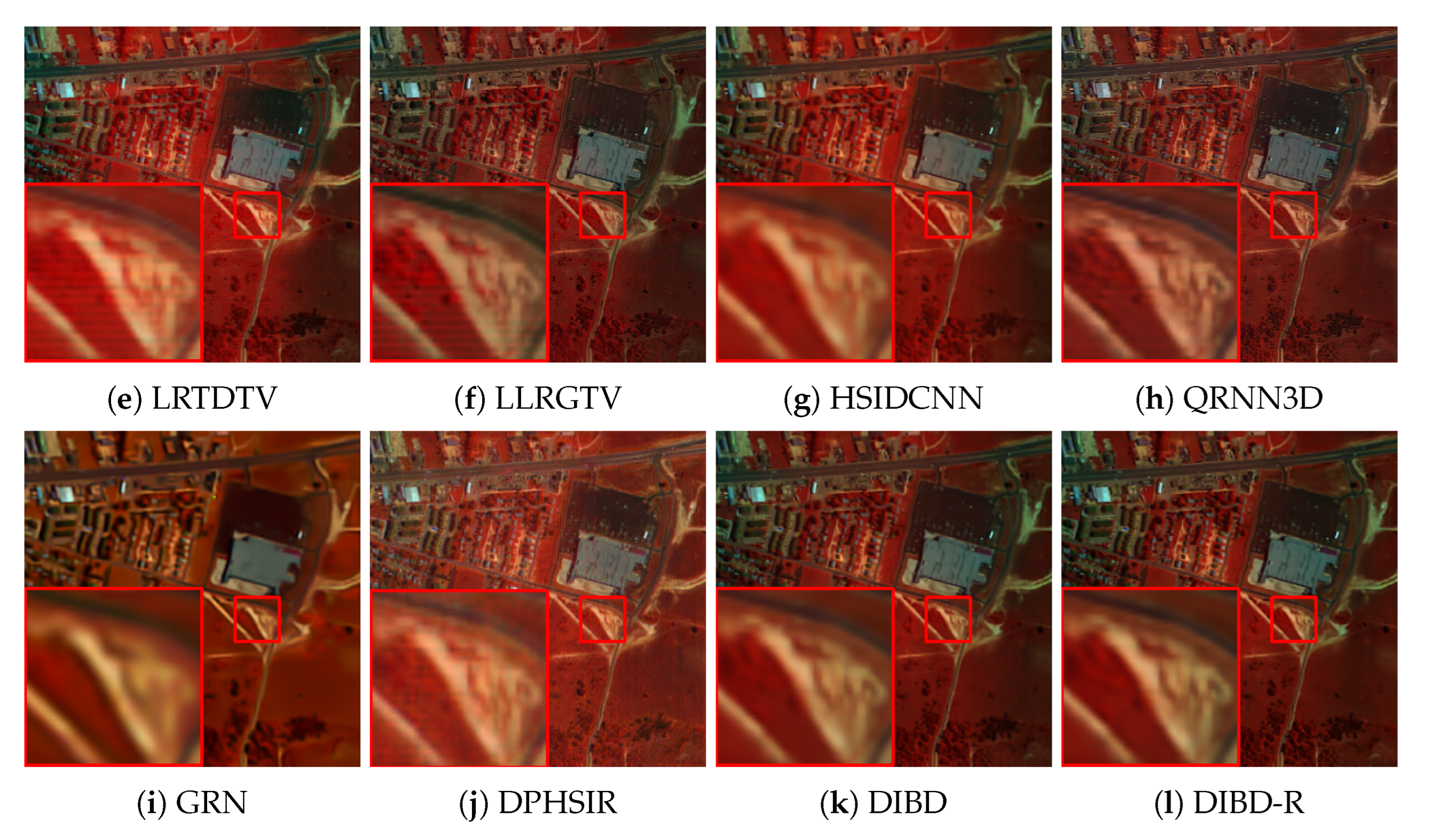
4.2.3. Real Noise Removal

To further confirm the effectiveness of our proposed DIBD in real noise removal, Indian Pines and Urban are selected for testing, which are severely polluted by the atmosphere, water absorption and complex noises. We employ two third stage’s trained models (i.e., whether trained with unlabeled real-world data) to evaluate, respectively. Specifically, from Figure 8, we can observe that all these comparison methods, except the NMoG and HSIDCNN, are unable to effectively remove the horizontal stripe noise, which is not contained in training data. The denoised result of the proposed DIBD training only with synthetic noise outperforms than others comparison methods. As mentioned before, the performance of subsequent tasks is seriously limited due to the quality of HSIs being severely deteriorated by various noises. Moreover, the visual effect cannot objectively reflect the denoising performance of each method. Therefore, we adopt the same classification algorithm to evaluate the quality of real-world denoised HSIs. The denoised and classification vision images of the Indian pines are presented in Figure 9. We can find in Table 7 that the proposed method’s overall accuracy (OA) achieves the best performance among the compared methods. From Figure 10, it can be observed that our DIBD achieves a sharper result than all compared methods. By contrast, the proposed DIBD training with unlabeled real data successfully tackles the most complex noise and generates clearer and sharper results on both the real-world datasets.
Overall, these experimental results indicate the effectiveness of our DIBD in generating higher quantitative evaluation and visually promising noiseless HSIs. Moreover, our proposed DIBD provides architecture interpretability and performance reliability under a Bayesian framework.

4.3. Ablation Study

We first conduct an ablation study to evaluate the impact of core modules of the proposed framework concerning DGExtractor and Degenerator. The first stage’s trained models are selected to evaluate the ICVL and CAVE datasets with higher noise intensity. We respectively add them to the baseline network, which contains only the Denoiser and Estimator. From Table 8, it can be easily seen that the baseline with DGExtractor and Degenerator achieves better performance than the other baselines. This is because the DGInfo learned by DGExtractor bears more information than the noise intensity, which eventually boosts the generalization ability. Moreover, the Degenerator provides additional supervision, which is helpful to learn the better mapping for the Denoiser.
Furthermore, the effect of our proposed strategies, i.e., the Degenerator on whether to adopt the priority dual regression scheme and the assistance of the DGInfo, is presented in Table 9. By fully considering the priority between different tasks and feeding the DGInfo to the Degenerator, the dual task can be handled effectively and the performance of whole network can be improved.

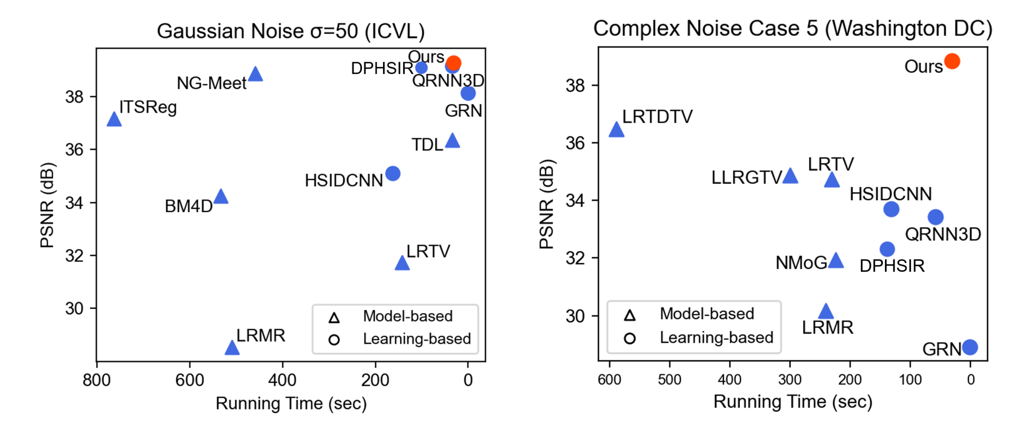
4.4. Efficiency Analysis

In this subsection, we mainly compare and analyze the efficiency of different learning-based methods in terms of inference time cost and model parameters on the ICVL and WDC datasets under noise case 5. The average inference time per image is measured on the Intel Xeon E5-2687W v4 CPU. The time cost and parameters comparison results with previous SOTA learning-based methods are shown in Table 10. As can be seen, the proposed DIBD performs much better than others with reasonable parameters and relatively less inference time. The proposed degradation information and dual regression scheme can promote the denoising model to remove noise in remotely sensed imagery or real-world HSI datasets. The evaluation results on the Washington DC datasets demonstrate the powerful generalization capability of DIBD. Thus, the proposed DIBD achieves a good trade-off between performance and efficiency.

4.5. Limitations Analysis

Although the proposed DIBD achieves superior denoising performance, there are still some limitations. Firstly, the learned degradation information significantly improves HSI denoising performance, but its design still lacks interpretation. In other words, the noise-relevant information and spatial-spectral correlation in HSIs can be extracted through the noisy HSI reconstruction process. However, the process of degradation information generation is difficult to control, and different physical knowledge embedding in degradation information is intractable to separate. One of our future research directions focuses on modeling the degradation information with accurate physical interpretation and achieving better performance in the same scenarios. Secondly, the proposed DIBD is constructed with 3D convolutional blocks, resulting in a sharp rise in parameters. Thus we consider constructing the light-weight model to alleviate this limitation as future work.

5. Conclusions

In this paper, we propose a novel Bayesian framework with degradation information learning for blind HSI denoising. We propose a priority dual learning algorithm to approximate the clean–noisy joint distribution appropriately. In addition, we develop comprehensive auxiliary information including noise intensity and implicit degradation information to guide the primary denoising and dual degenerating tasks. Extensive experiments on synthetic and real-world data demonstrate the superiority and generalization of the proposed method.

Author Contributions

Conceptualization, X.W. and Y.G.; methodology, X.W. and J.X.; software, J.X.; validation, J.X.; formal analysis, X.W.; investigation, X.W.; resources, Y.G.; data curation, J.X.; writing—original draft preparation, X.W. and J.X.; writing—review and editing, X.W. and Y.G.; visualization, J.X.; supervision, Y.G.; project administration, X.W.; funding acquisition, X.W. All authors have read and agreed to the published version of the manuscript.

Funding

This research was funded by National Key Research and Development Project of China grant number 2020AAA0105600, National Natural Science Foundation of China grant number 62006183, and Fundamental Research Funds for the Central Universities under grant Numbers xhj032021017-04.

Data Availability Statement

Not applicable.

Acknowledgments

The authors would like to thank Xiangyong Cao for discussions.

Conflicts of Interest

The authors declare no conflict of interest. The funders had no role in the design of the study; in the collection, analyses, or interpretation of data; in the writing of the manuscript; or in the decision to publish the results.

Abbreviations

The following abbreviations are used in this manuscript:
HSIHyperspectral image
CNNConvolutional neural network
GANGenerative adversarial network
WDCWashington DC Mall HSI dataset
BM4DBlock matching with 4D filtering
LRMRLow-rank matrix recovery
LRTVTotal variation regularized low-rank matrix factorization
NMoGThe non-iid mixture of Gaussian
LRTDTVTotal variation regularized low-rank tensor decomposition
LLRGTVLocal low-rank matrix recovery and global spatial–spectral total variation
NGMeetNon-local meets global
TDLTensor dictionary learning
HSI-DeNetHyperspectral image restoration via convolutional neural network
HSIDCNNHyperspectral image denoising employing
a spatial–spectral deep residual convolutional neural network
QRNN3D3D quasi-recurrent neural network
GRNGlobal reasoning network
DPHSIRDeep plug-and-play prior for hyperspectral image restoration
BBand
HHeight
WWidth
PSNRPeak signal-to-noise ratio
SSIMStructural similarity
SAMSpectral angle mapper

References

  1. Yu, C.; Han, R.; Song, M.; Liu, C.; Chang, C.I. Feedback attention-based dense CNN for hyperspectral image classification. IEEE Trans. Geosci. Remote Sens. 2021, 60, 5501916. [Google Scholar] [CrossRef]
  2. Sun, X.; Qu, Y.; Gao, L.; Sun, X.; Qi, H.; Zhang, B.; Shen, T. Ensemble-based information retrieval with mass estimation for hyperspectral target detection. IEEE Trans. Geosci. Remote Sens. 2021, 60, 5508123. [Google Scholar] [CrossRef]
  3. Song, M.; Shang, X.; Chang, C.I. 3-D receiver operating characteristic analysis for hyperspectral image classification. IEEE Trans. Geosci. Remote Sens. 2020, 58, 8093–8115. [Google Scholar] [CrossRef]
  4. Zhao, L.; Luo, W.; Liao, Q.; Chen, S.; Wu, J. Hyperspectral Image Classification with Contrastive Self-Supervised Learning Under Limited Labeled Samples. IEEE Geosci. Remote Sens. Lett. 2022, 19, 6008205. [Google Scholar] [CrossRef]
  5. Ji, Y.; Jiang, P.; Guo, Y.; Zhang, R.; Wang, F. Self-paced collaborative representation with manifold weighting for hyperspectral anomaly detection. Remote Sens. Lett. 2022, 13, 599–610. [Google Scholar] [CrossRef]
  6. Xie, Q.; Zhao, Q.; Meng, D.; Xu, Z.; Gu, S.; Zuo, W.; Zhang, L. Multispectral images denoising by intrinsic tensor sparsity regularization. In Proceedings of the IEEE Conference on Computer Vision and Pattern Recognition, Las Vegas, NV, USA, 26 June–1 July 2016; pp. 1692–1700. [Google Scholar]
  7. Chang, Y.; Yan, L.; Zhong, S. Hyper-laplacian regularized unidirectional low-rank tensor recovery for multispectral image denoising. In Proceedings of the IEEE Conference on Computer Vision and Pattern Recognition, Honolulu, HI, USA, 21–26 July 2017; pp. 4260–4268. [Google Scholar]
  8. He, W.; Yao, Q.; Li, C.; Yokoya, N.; Zhao, Q. Non-local meets global: An integrated paradigm for hyperspectral denoising. In Proceedings of the IEEE/CVF Conference on Computer Vision and Pattern Recognition, Long Beach, CA, USA, 15–20 June 2019; pp. 6868–6877. [Google Scholar]
  9. Kong, X.; Zhao, Y.; Xue, J.; Chan, J.C.W.; Ren, Z.; Huang, H.; Zang, J. Hyperspectral image denoising based on nonlocal low-rank and TV regularization. Remote Sens. 2020, 12, 1956. [Google Scholar] [CrossRef]
  10. Chen, Y.; Cao, X.; Zhao, Q.; Meng, D.; Xu, Z. Denoising hyperspectral image with non-iid noise structure. IEEE Trans. Cybern. 2017, 48, 1054–1066. [Google Scholar] [CrossRef] [Green Version]
  11. Wang, Y.; Peng, J.; Zhao, Q.; Leung, Y.; Zhao, X.L.; Meng, D. Hyperspectral image restoration via total variation regularized low-rank tensor decomposition. IEEE J. Sel. Top. Appl. Earth Obs. Remote Sens. 2017, 11, 1227–1243. [Google Scholar] [CrossRef] [Green Version]
  12. He, W.; Zhang, H.; Shen, H.; Zhang, L. Hyperspectral image denoising using local low-rank matrix recovery and global spatial–spectral total variation. IEEE J. Sel. Top. Appl. Earth Obs. Remote Sens. 2018, 11, 713–729. [Google Scholar] [CrossRef]
  13. Sun, L.; Zhan, T.; Wu, Z.; Xiao, L.; Jeon, B. Hyperspectral mixed denoising via spectral difference-induced total variation and low-rank approximation. Remote Sens. 2018, 10, 1956. [Google Scholar] [CrossRef]
  14. Zhuang, L.; Ng, M.K.; Fu, X. Hyperspectral Image Mixed Noise Removal Using Subspace Representation and Deep CNN Image Prior. Remote Sens. 2021, 13, 4098. [Google Scholar] [CrossRef]
  15. Zhang, T.; Fu, Y.; Li, C. Hyperspectral image denoising with realistic data. In Proceedings of the IEEE/CVF International Conference on Computer Vision, Montreal, QC, Canada, 11–17 October 2021; pp. 2248–2257. [Google Scholar]
  16. Yuan, Q.; Zhang, Q.; Li, J.; Shen, H.; Zhang, L. Hyperspectral image denoising employing a spatial–spectral deep residual convolutional neural network. IEEE Trans. Geosci. Remote Sens. 2018, 57, 1205–1218. [Google Scholar] [CrossRef] [Green Version]
  17. Wei, K.; Fu, Y.; Huang, H. 3-D quasi-recurrent neural network for hyperspectral image denoising. IEEE Trans. Neural Netw. Learn. Syst. 2020, 32, 363–375. [Google Scholar] [CrossRef] [Green Version]
  18. Cao, X.; Fu, X.; Xu, C.; Meng, D. Deep spatial-spectral global reasoning network for hyperspectral image denoising. IEEE Trans. Geosci. Remote Sens. 2021, 60, 5504714. [Google Scholar] [CrossRef]
  19. Zhang, J.; Cai, Z.; Chen, F.; Zeng, D. Hyperspectral Image Denoising via Adversarial Learning. Remote Sens. 2022, 14, 1790. [Google Scholar] [CrossRef]
  20. Pang, L.; Gu, W.; Cao, X. TRQ3DNet: A 3D Quasi-Recurrent and Transformer Based Network for Hyperspectral Image Denoising. Remote Sens. 2022, 14, 4598. [Google Scholar] [CrossRef]
  21. Maffei, A.; Haut, J.M.; Paoletti, M.E.; Plaza, J.; Bruzzone, L.; Plaza, A. A single model CNN for hyperspectral image denoising. IEEE Trans. Geosci. Remote Sens. 2019, 58, 2516–2529. [Google Scholar] [CrossRef]
  22. Yuan, Y.; Ma, H.; Liu, G. Partial-DNet: A novel blind denoising model with noise intensity estimation for HSI. IEEE Trans. Geosci. Remote Sens. 2021, 60, 5505913. [Google Scholar] [CrossRef]
  23. Lai, Z.; Wei, K.; Fu, Y. Deep plug-and-play prior for hyperspectral image restoration. Neurocomputing 2022, 481, 281–293. [Google Scholar] [CrossRef]
  24. Xiong, F.; Zhou, J.; Zhao, Q.; Lu, J.; Qian, Y. MAC-Net: Model-Aided Nonlocal Neural Network for Hyperspectral Image Denoising. IEEE Trans. Geosci. Remote Sens. 2021, 60, 5519414. [Google Scholar] [CrossRef]
  25. Yue, Z.; Zhao, Q.; Zhang, L.; Meng, D. Dual adversarial network: Toward real-world noise removal and noise generation. In Proceedings of the European Conference on Computer Vision, Glasgow, UK, 23–28 August 2020; Springer: Berlin/Heidelberg, Germany, 2020; pp. 41–58. [Google Scholar]
  26. Zheng, D.; Zhang, X.; Ma, K.; Bao, C. Learn from Unpaired Data for Image Restoration: A Variational Bayes Approach. arXiv 2022, arXiv:2204.10090. [Google Scholar] [CrossRef] [PubMed]
  27. Chen, J.; Chen, J.; Chao, H.; Yang, M. Image blind denoising with generative adversarial network based noise modeling. In Proceedings of the IEEE Conference on Computer Vision and Pattern Recognition, Salt Lake City, UT, USA, 18–23 June 2018; pp. 3155–3164. [Google Scholar]
  28. Kim, D.W.; Ryun Chung, J.; Jung, S.W. Grdn: Grouped residual dense network for real image denoising and gan-based real-world noise modeling. In Proceedings of the IEEE/CVF Conference on Computer Vision and Pattern Recognition Workshops, Long Beach, CA, USA, 16–17 June 2019. [Google Scholar]
  29. He, D.; Xia, Y.; Qin, T.; Wang, L.; Yu, N.; Liu, T.Y.; Ma, W.Y. Dual learning for machine translation. Adv. Neural Inf. Process. Syst. 2016, 29. [Google Scholar]
  30. Yi, Z.; Zhang, H.; Tan, P.; Gong, M. Dualgan: Unsupervised dual learning for image-to-image translation. In Proceedings of the IEEE International Conference on Computer Vision, Venice, Italy, 22–29 October 2017; pp. 2849–2857. [Google Scholar]
  31. Zhu, J.Y.; Park, T.; Isola, P.; Efros, A.A. Unpaired image-to-image translation using cycle-consistent adversarial networks. In Proceedings of the IEEE International Conference on Computer Vision, Venice, Italy, 22–29 October 2017; pp. 2223–2232. [Google Scholar]
  32. Guo, Y.; Chen, J.; Wang, J.; Chen, Q.; Cao, J.; Deng, Z.; Xu, Y.; Tan, M. Closed-loop matters: Dual regression networks for single image super-resolution. In Proceedings of the IEEE/CVF Conference on Computer Vision and Pattern Recognition, Seattle, WA, USA, 13–19 June 2020; pp. 5407–5416. [Google Scholar]
  33. Hu, X.; Cai, Y.; Liu, Z.; Wang, H.; Zhang, Y. Multi-Scale Selective Feedback Network with Dual Loss for Real Image Denoising. In Proceedings of the IJCAI, Montreal, QC, Canada, 19–27 August 2021; pp. 729–735. [Google Scholar]
  34. Zhang, K.; Zuo, W.; Chen, Y.; Meng, D.; Zhang, L. Beyond a gaussian denoiser: Residual learning of deep cnn for image denoising. IEEE Trans. Image Process. 2017, 26, 3142–3155. [Google Scholar] [CrossRef] [PubMed] [Green Version]
  35. Zhang, K.; Zuo, W.; Zhang, L. FFDNet: Toward a fast and flexible solution for CNN-based image denoising. IEEE Trans. Image Process. 2018, 27, 4608–4622. [Google Scholar] [CrossRef] [PubMed] [Green Version]
  36. Guo, S.; Yan, Z.; Zhang, K.; Zuo, W.; Zhang, L. Toward convolutional blind denoising of real photographs. In Proceedings of the IEEE/CVF Conference on Computer Vision and Pattern Recognition, Long Beach, CA, USA, 15–20 June 2019; pp. 1712–1722. [Google Scholar]
  37. Gou, Y.; Hu, P.; Lv, J.; Peng, X. Multi-Scale Adaptive Network for Single Image Denoising. arXiv 2022, arXiv:2203.04313. [Google Scholar]
  38. Li, B.; Gou, Y.; Gu, S.; Liu, J.Z.; Zhou, J.T.; Peng, X. You only look yourself: Unsupervised and untrained single image dehazing neural network. Int. J. Comput. Vis. 2021, 129, 1754–1767. [Google Scholar] [CrossRef]
  39. Maggioni, M.; Katkovnik, V.; Egiazarian, K.; Foi, A. Nonlocal transform-domain filter for volumetric data denoising and reconstruction. IEEE Trans. Image Process. 2012, 22, 119–133. [Google Scholar] [CrossRef]
  40. Peng, Y.; Meng, D.; Xu, Z.; Gao, C.; Yang, Y.; Zhang, B. Decomposable nonlocal tensor dictionary learning for multispectral image denoising. In Proceedings of the IEEE Conference on Computer Vision and Pattern Recognition, Columbus, OH, USA, 23–28 June 2014; pp. 2949–2956. [Google Scholar]
  41. Zhang, H.; He, W.; Zhang, L.; Shen, H.; Yuan, Q. Hyperspectral image restoration using low-rank matrix recovery. IEEE Trans. Geosci. Remote Sens. 2013, 52, 4729–4743. [Google Scholar] [CrossRef]
  42. He, W.; Zhang, H.; Zhang, L.; Shen, H. Total-variation-regularized low-rank matrix factorization for hyperspectral image restoration. IEEE Trans. Geosci. Remote Sens. 2015, 54, 178–188. [Google Scholar] [CrossRef]
  43. Chang, Y.; Yan, L.; Fang, H.; Zhong, S.; Liao, W. HSI-DeNet: Hyperspectral image restoration via convolutional neural network. IEEE Trans. Geosci. Remote Sens. 2018, 57, 667–682. [Google Scholar] [CrossRef]
  44. Dong, W.; Wang, H.; Wu, F.; Shi, G.; Li, X. Deep spatial–spectral representation learning for hyperspectral image denoising. IEEE Trans. Comput. Imaging 2019, 5, 635–648. [Google Scholar] [CrossRef]
  45. Liu, W.; Lee, J. A 3-D atrous convolution neural network for hyperspectral image denoising. IEEE Trans. Geosci. Remote Sens. 2019, 57, 5701–5715. [Google Scholar] [CrossRef]
  46. Goodfellow, I.; Pouget-Abadie, J.; Mirza, M.; Xu, B.; Warde-Farley, D.; Ozair, S.; Courville, A.; Bengio, Y. Generative adversarial networks. Commun. ACM 2020, 63, 139–144. [Google Scholar] [CrossRef]
  47. Li, B.; Liu, X.; Hu, P.; Wu, Z.; Lv, J.; Peng, X. All-In-One image restoration for unknown corruption. In Proceedings of the IEEE/CVF Conference on Computer Vision and Pattern Recognition, New Orleans, LA, USA, 19–20 June 2022; pp. 17452–17462. [Google Scholar]
  48. Liu, X.; Tanaka, M.; Okutomi, M. Single-image noise level estimation for blind denoising. IEEE Trans. Image Process. 2013, 22, 5226–5237. [Google Scholar] [CrossRef]
  49. Kingma, D.P.; Welling, M. Auto-encoding variational bayes. arXiv 2013, arXiv:1312.6114. [Google Scholar]
  50. Ronneberger, O.; Fischer, P.; Brox, T. U-net: Convolutional networks for biomedical image segmentation. In Proceedings of the International Conference on Medical Image Computing and Computer-Assisted Intervention, Munich, Germany, 5–9 October 2015; Springer: Berlin/Heidelberg, Germany, 2015; pp. 234–241. [Google Scholar]
  51. Zhang, Y.; Tian, Y.; Kong, Y.; Zhong, B.; Fu, Y. Residual dense network for image super-resolution. In Proceedings of the IEEE Conference on Computer Vision and Pattern Recognition, Salt Lake City, UT, USA, 18–23 June 2018; pp. 2472–2481. [Google Scholar]
  52. Arad, B.; Ben-Shahar, O. Sparse recovery of hyperspectral signal from natural RGB images. In Proceedings of the European Conference on Computer Vision, Amsterdam, The Netherlands, 11–14 October 2016; Springer: Berlin/Heidelberg, Germany, 2016; pp. 19–34. [Google Scholar]
  53. Gamba, P. A collection of data for urban area characterization. In Proceedings of the IGARSS 2004, 2004 IEEE International Geoscience and Remote Sensing Symposium, Anchorage, AK, USA, 20–24 September 2004; Volume 1. [Google Scholar]
  54. Landgrebe, D.A. Signal Theory Methods in Multispectral Remote Sensing; John Wiley & Sons: Hoboken, NJ, USA, 2003; Volume 24. [Google Scholar]
  55. Mnih, V.; Hinton, G.E. Learning to detect roads in high-resolution aerial images. In Proceedings of the European Conference on Computer Vision, Crete, Greece, 5–11 September 2010; Springer: Berlin/Heidelberg, Germany, 2010; pp. 210–223. [Google Scholar]
  56. Park, J.I.; Lee, M.H.; Grossberg, M.D.; Nayar, S.K. Multispectral imaging using multiplexed illumination. In Proceedings of the 2007 IEEE 11th International Conference on Computer Vision, Rio De Janeiro, Brazil, 14–21 October 2007; pp. 1–8. [Google Scholar]
  57. Wang, Z.; Bovik, A.C.; Sheikh, H.R.; Simoncelli, E.P. Image quality assessment: From error visibility to structural similarity. IEEE Trans. Image Process. 2004, 13, 600–612. [Google Scholar] [CrossRef]
  58. Yuhas, R.H.; Boardman, J.W.; Goetz, A.F. Determination of semi-arid landscape endmembers and seasonal trends using convex geometry spectral unmixing techniques. In Proceedings of the JPL, Summaries of the 4th Annual JPL Airborne Geoscience Workshop, Washington, DC, USA, 25–28 October 1993; Volume 1. [Google Scholar]
  59. Kingma, D.P.; Ba, J. Adam: A method for stochastic optimization. arXiv 2014, arXiv:1412.6980. [Google Scholar]
Figure 1. Quantitative comparisons (PSNR (dB) vs. running speed (second)) of our DIBD against other competitive approaches on the ICVL and Washington DC datasets.
Remotesensing 15 00490 g001
Figure 2. Overview of our DIBD framework.
Remotesensing 15 00490 g002
Figure 3. Denoising results (PSNR, dB) and visual comparison of the image from the ICVL dataset under the AWGN intensity σ = 50. The RGB image is synthesized by HSI bands 23, 12, 9.
Remotesensing 15 00490 g003
Figure 4. Denoising results (PSNR, dB) and visual comparison of the image from the ICVL dataset under the complex case 5. The RGB image is synthesized by HSI bands 21, 11, 6.
Remotesensing 15 00490 g004
Figure 5. Denoising results (PSNR, dB) and visual comparison of the image from ICVL dataset under noise case 5. The RGB image is synthesized by HSI bands 8, 18, 28.
Remotesensing 15 00490 g005
Figure 6. Denoising results (PSNR, dB) and visual comparisons of the image from the Washington DC dataset under complex noise of case 5. The RGB image is synthesized by HSI bands 78, 45, 12.
Remotesensing 15 00490 g006
Figure 7. PSNR curves of each band for the images shown Figure 6.
Remotesensing 15 00490 g007
Figure 8. Pavia university denoising results. The RGB image is synthesized by HSI bands 78, 3, 2.
Remotesensing 15 00490 g008
Figure 9. Classification quantitative (OA) and qualitative results of Indian Pines dataset. DIBD-R denotes DIBD training on both labeled and unlabeled mixed data. The RGB image is synthesized by HSI bands 28, 4, 2.
Remotesensing 15 00490 g009aRemotesensing 15 00490 g009b
Figure 10. Urban denoising results. DIBD-R denotes DIBD training on both labeled and unlabeled mixed data. The RGB image is synthesized by HSI bands 104, 54, 24.
Remotesensing 15 00490 g010aRemotesensing 15 00490 g010b
Table 1. Network configuration of the denoiser.
ModuleLayersKernel SizeStrideInput SizeOutput Size
Block 1Conv3d, ReLU3 × 3 × 31 × 1 × 13 × B × H × W64 × B × H × W
Conv3d, ReLU3 × 3 × 31 × 1 × 164 × B × H × W64 × B × H × W
Block 2Conv3d1 × 2 × 21 × 2 × 264 × B × H × W64 × B × H 2 × W 2
Block 3Conv3d, ReLU3 × 3 × 31 × 1 × 164 × B × H 2 × W 2 128 × B × H 2 × W 2
RDB3d3 × 3 × 31 × 1 × 1128 × B × H 2 × W 2 128 × B × H 2 × W 2
Block 4Conv3d1 × 2 × 21 × 2 × 2128 × B × H 2 × W 2 128 × B × H 4 × W 4
Block 5Conv3d, ReLU3 × 3 × 31 × 1 × 1128 × B × H 4 × W 4 256 × B × H 4 × W 4
RDB3d3 × 3 × 31 × 1 × 1256 × B × H 4 × W 4 256 × B × H 4 × W 4
Block 6ConvTranspose3d1 × 2 × 21 × 2 × 2256 × B × H 4 × W 4 256 × B × H 2 × W 2
Block 7Conv3d, ReLU3 × 3 × 31 × 1 × 1256 × B × H 2 × W 2 128 × B × H 2 × W 2
RDB3d3 × 3 × 31 × 1 × 1128 × B × H 2 × W 4 128 × B × H 2 × W 2
Block 8ConvTranspose3d1 × 2 × 21 × 2 × 2128 × B × H 2 × W 2 128 × B × H × W
Block 9Conv3d, ReLU3 × 3 × 31 × 1 × 1128 × B × H × W64 × B × H × W
RDB3d3 × 3 × 31 × 1 × 164 × B × H × W64 × B × H × W
OutputConv3d3 × 3 × 31 × 1 × 164 × B × H × W1 × B × H × W
Table 2. Network configuration of the degenerator.
ModuleLayersKernel SizeStrideInput SizeOutput Size
Conv3d, LeakyReLU3 × 3 × 31 × 1 × 13 × B × H × W32 × B × H × W
Block 1Conv3d3 × 3 × 31 × 1 × 132 × B × H × W32 × B × H × W
Conv3d1 × 1 × 11 × 1 × 132 × B × H × W32 × B × H × W
Conv3d, LeakyReLU3 × 3 × 31 × 1 × 132 × B × H × W32 × B × H × W
Block 2Conv3d3 × 3 × 31 × 1 × 132 × B × H × W32 × B × H × W
Conv3d1 × 1 × 11 × 1 × 132 × B × H × W1 × B × H × W
Table 3. Network configuration of the encoder.
ModuleLayersKernel SizeStrideInput SizeOutput Size
Block 1Conv3d, LeakyReLU3 × 3 × 31 × 1 × 11 × B × H × W32 × B × H × W
Block 2Conv3d1 × 2 × 21 × 2 × 232 × B × H × W32 × B × H 2 × W 2
Conv3d, LeakyReLU3 × 3 × 31 × 1 × 132 × B × H 2 × W 2 32 × B × H 2 × W 2
Block 3Conv3d1 × 2 × 21 × 2 × 232 × B × H × W32 × B × H 4 × W 4
Conv3d, LeakyReLU3 × 3 × 31 × 1 × 132 × B × H 4 × W 4 32 × B × H 4 × W 4
Block 4 (a)Conv3d, LeakyReLU3 × 3 × 31 × 1 × 132 × B × H 4 × W 4 32 × B × H 4 × W 4
μ , input (a)Conv3d1 × 2 × 21 × 2 × 232 × B × H 4 × W 4 1 × B × H 4 × W 4
log ς 2 , input (a)Conv3d1 × 2 × 21 × 2 × 232 × B × H 4 × W 4 1 × B × H 4 × W 4
Table 4. Network configuration of the decoder.
ModuleLayersKernel SizeStrideInput SizeOutput Size
Block 1Conv3d, LeakyReLU3 × 3 × 31 × 1 × 11 × B × H 4 × W 4 32 × B × H 4 × W 4
Block 2Conv3d, LeakyReLU3 × 3 × 31 × 1 × 132 × B × H 4 × W 4 32 × B × H 4 × W 4
ConvTranspose3d1 × 2 × 21 × 2 × 232 × B × H 4 × W 4 32 × B × H 2 × W 2
Block 3Conv3d, LeakyReLU3 × 3 × 31 × 1 × 132 × B × H 2 × W 2 32 × B × H 2 × W 2
ConvTranspose3d1 × 2 × 21 × 2 × 232 × B × H 2 × W 2 32 × B × H × W
OutputConv3d, LeakyReLU3 × 3 × 31 × 1 × 132 × B × H × W1 × B × H × W
Table 5. Quantitative evaluation of all the competing methods under different Gaussian noise intensities on ICVL dataset.
MethodsBlind/Non-Blind σ = 30 σ = 50 σ = 70Blind
PSNRSSIMSAMPSNRSSIMSAMPSNRSSIMSAMPSNRSSIMSAM
Noisy18.590.08490.824614.150.03290.995811.230.01691.106314.210.03620.9946
BM4D [39]Non-blind39.360.93590.144536.510.88800.208634.580.84070.254436.500.88510.2108
LRMR [41]Blind34.000.70110.313430.020.51200.415127.190.38170.499830.040.51390.4129
LRTV [42]Blind37.950.91790.161335.670.87980.211834.120.84520.253734.550.89730.1090
TDL [40]Non-blind42.210.96200.071139.790.93900.108738.060.91560.139039.780.93760.1668
ITSReg [6]Non-blind42.280.95080.157140.010.92650.183138.210.91160.201339.980.92940.1745
NG-Meet [8]Non-blind43.340.95540.054040.640.94010.066839.050.92900.076940.770.94120.0674
HSIDCNN [16]Blind40.100.95380.111837.430.92420.147135.420.88970.178437.350.92200.1493
QRNN3D [17]Blind43.860.97610.065941.710.96400.082539.570.94520.113341.540.96270.0870
GRN [18]Blind40.970.97220.084539.760.96180.093338.380.94510.105139.630.96040.0947
DPHSIR [23]Non-blind44.700.97820.057442.110.96460.077638.500.91930.151939.250.88600.1310
DIBDBlind44.370.97710.059042.080.96490.074740.520.95390.089742.070.96480.0750
Table 6. Quantitative evaluation of all the competing methods under different complex noise cases on the ICVL dataset. All denoising methods work in the blind way.
MethodsCase 1Case 2Case 3Case 4Case 5
PSNRSSIMSAMPSNRSSIMSAMPSNRSSIMSAMPSNRSSIMSAMPSNRSSIMSAM
Noisy17.770.14280.867817.650.13860.868417.560.13850.880614.880.10240.91113.820.07920.9271
LRMR32.980.68340.264332.890.68110.264032.220.68230.298830.680.61850.336329.750.59170.3781
LRTV33.610.89100.109533.580.88720.116132.280.88060.127028.540.68330.477927.220.66750.4963
NMoG35.050.83530.226833.800.77390.428432.900.77520.398529.480.67280.556227.160.58830.5677
LRTDTV35.590.91360.126535.640.91400.123634.950.91470.121434.800.90790.133433.580.90380.1351
LLRGTV35.760.87680.211035.750.87370.219534.290.85380.272233.820.83970.384131.870.81270.3949
HSIDCNN39.050.94340.107938.700.94120.104938.540.93950.104936.570.90550.140435.300.88740.1532
QRNN3D44.000.97940.050443.660.97830.051743.620.97840.051042.630.97100.071441.160.96340.0810
GRN38.790.95980.072038.680.95900.072538.760.95860.072534.510.88910.428034.680.89500.1535
DPHSIR44.140.97960.045843.710.97800.048043.580.97830.047042.470.97110.064139.570.95960.0797
DIBD44.920.98230.043644.690.98150.044844.740.98160.044643.860.97760.050042.250.97020.0614
Table 7. Classification quantitative result on Indian Pines dataset. DIBD-R denotes DIBD training on paired and unlabeled mixed data.
MetricsNoisyBM4DLRMRLRTVNMoGLRTDTVHSIDCNNQRNN3DGRNDPHSIRDIBDDIBD-R
OA78.0684.4081.3881.2980.7383.3790.1390.1990.2778.7091.8392.50
Kappa0.74630.82070.78620.78450.77870.80880.88720.88760.88870.75360.90670.9144
Table 8. Ablation study on DGExtractor and Degenerator.
ICVL with σ = 70CAVE with σ = 95
Baseline
Degenerator
DGExtractor
PSNR31.7432.8635.0236.3326.2026.7428.4629.27
SSIM0.62970.68040.77770.84300.44420.46020.60290.6361
SAM0.26700.22450.13450.13220.63630.51160.41220.4470
Params (#)3.16M3.25M3.32M3.41M3.16M3.25M3.32M3.41M
Table 9. Ablation study on training strategies. Priority-DR denotes priority dual regression strategy. Degenerator-DG denotes the Degenerator is trained with DGInfo.
ICVL with σ = 70CAVE with σ = 95
Priority-DR
Degenerator-DG
PSNR34.6236.3336.5428.4329.2729.90
SSIM0.76890.84300.84500.57080.63610.6832
SAM0.15380.13220.12030.52470.44700.3796
Table 10. The efficiency comparisons of previous SOTA learning-based methods and DIBD on the ICVL and Washington DC datasets.
MethodsParams (M)ICVLWDC
PSNR (dB)Time Cost (s)PSNR (dB)Time Cost (s)
HSIDCNN0.3735.30183.6233.71119.54
QRNN3D0.8641.1633.2533.4267.14
GRN1.0634.6810.4328.925.41
DPHSIR14.2739.57112.6732.16123.36
DIBD3.4142.2530.8338.8424.47
Disclaimer/Publisher’s Note: The statements, opinions and data contained in all publications are solely those of the individual author(s) and contributor(s) and not of MDPI and/or the editor(s). MDPI and/or the editor(s) disclaim responsibility for any injury to people or property resulting from any ideas, methods, instructions or products referred to in the content.

