
Analysis of Space-Based Observed Infrared Characteristics of Aircraft in the Air
 and
and
Abstract
:1. Introduction
2. Methods and Materials
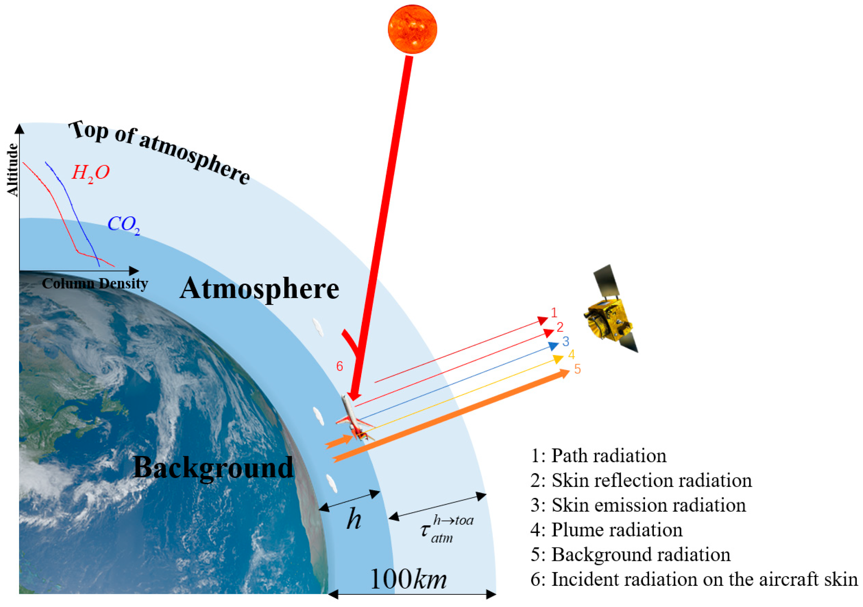
2.1. Observed Radiance of Aircraft by Space-based Sensor
2.2. The Flow and Metrics of Analysis
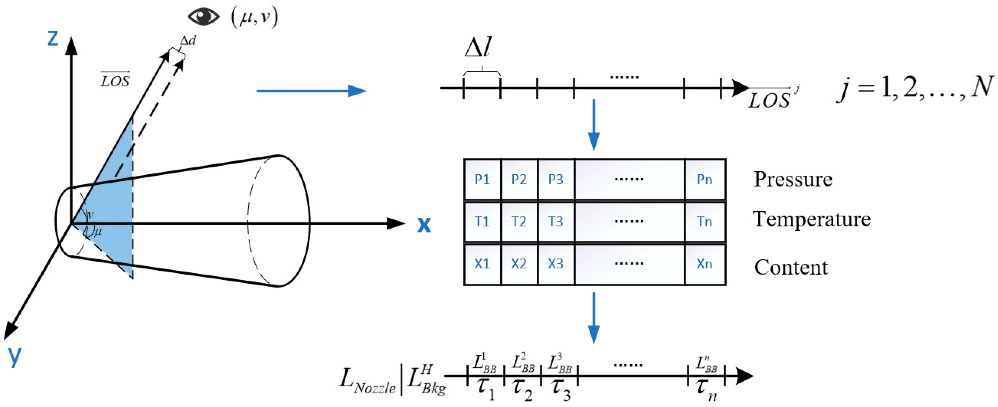
2.3. Simulation Modeling
2.3.1. Skin Radiance
2.3.2. Plume Radiance
2.3.3. Background Radiation Calculation and Instrument Performance Simulation
2.4. Materials for Simulation Case Study
3. Results
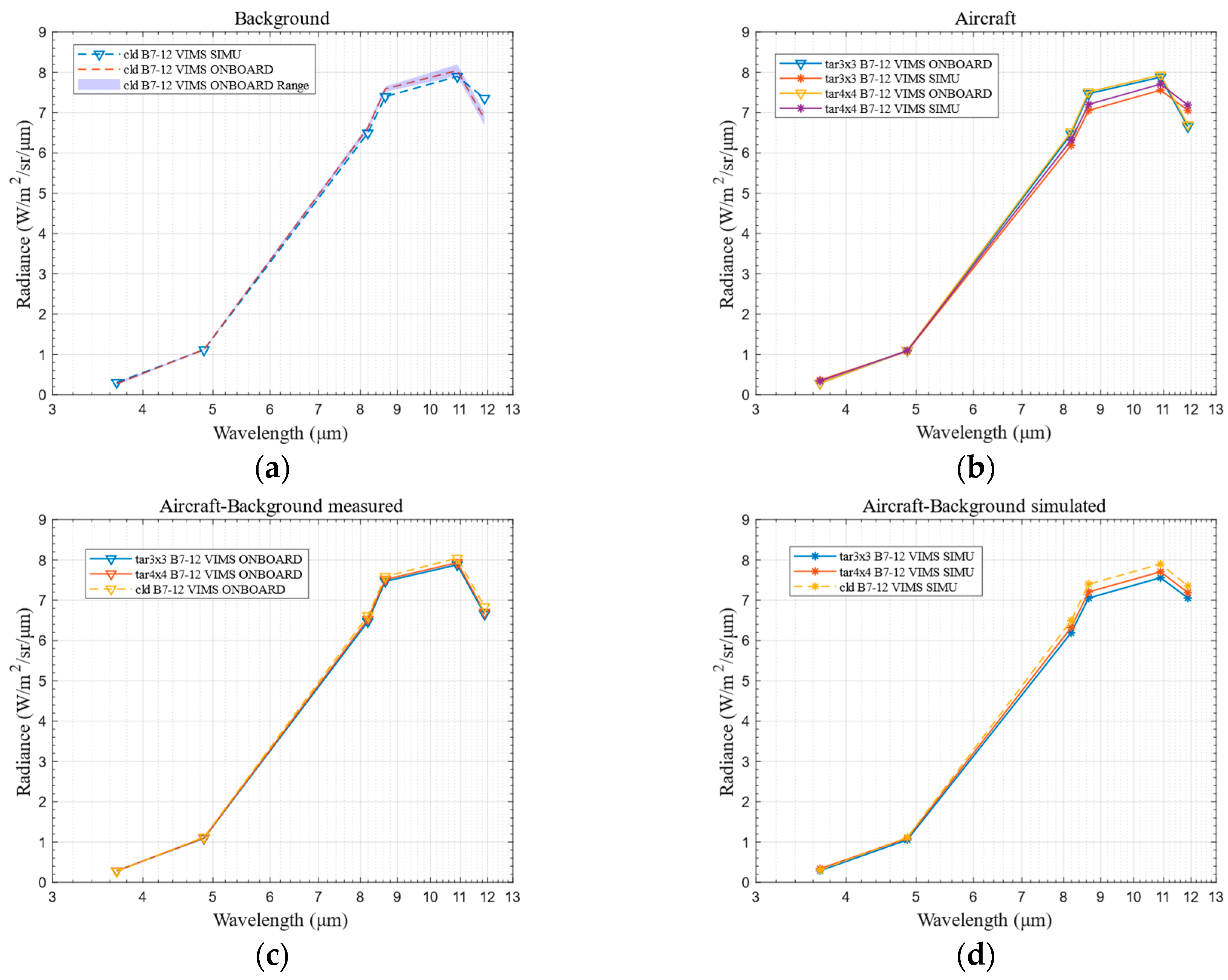
3.1. Validation of the Simulation Results
3.1.1. Space-Based Simulation Validation
3.1.2. Plume Simulation Validation
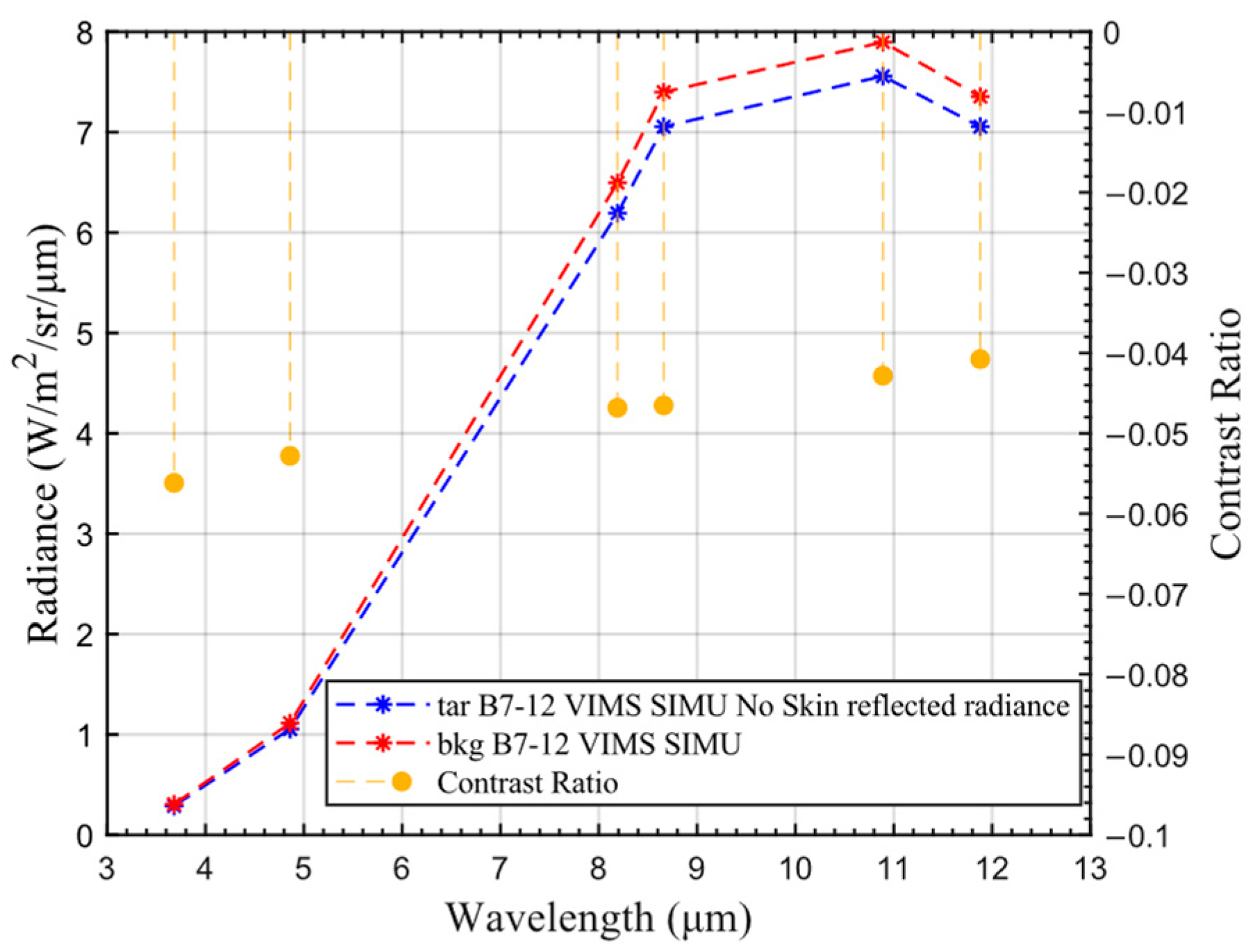
3.2. Evaluation of the Aircraft and Background Contribution to the Observed Radiance
3.3. Analysis of the Effect of Instrument Performance on Target-Background Contrast
4. Discussions
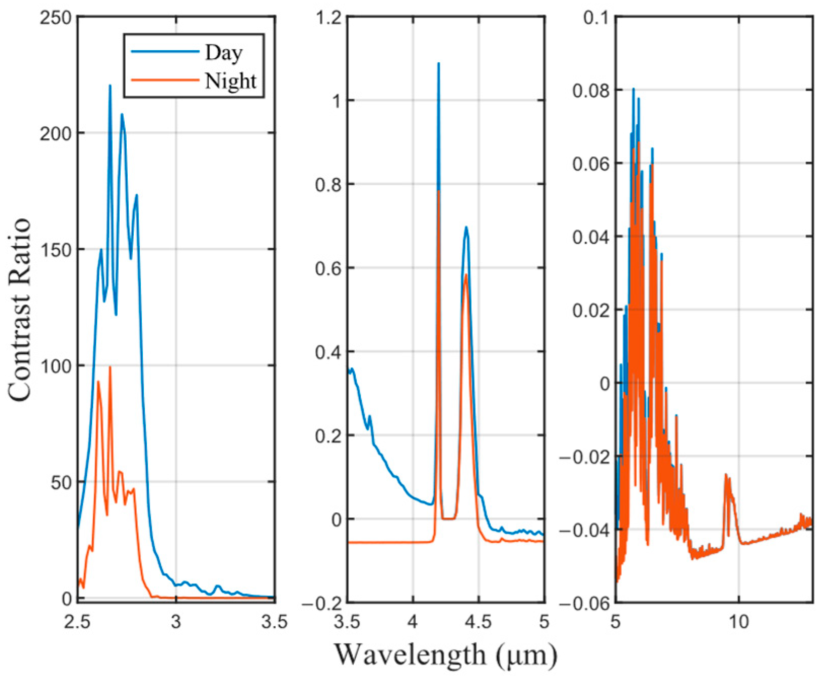
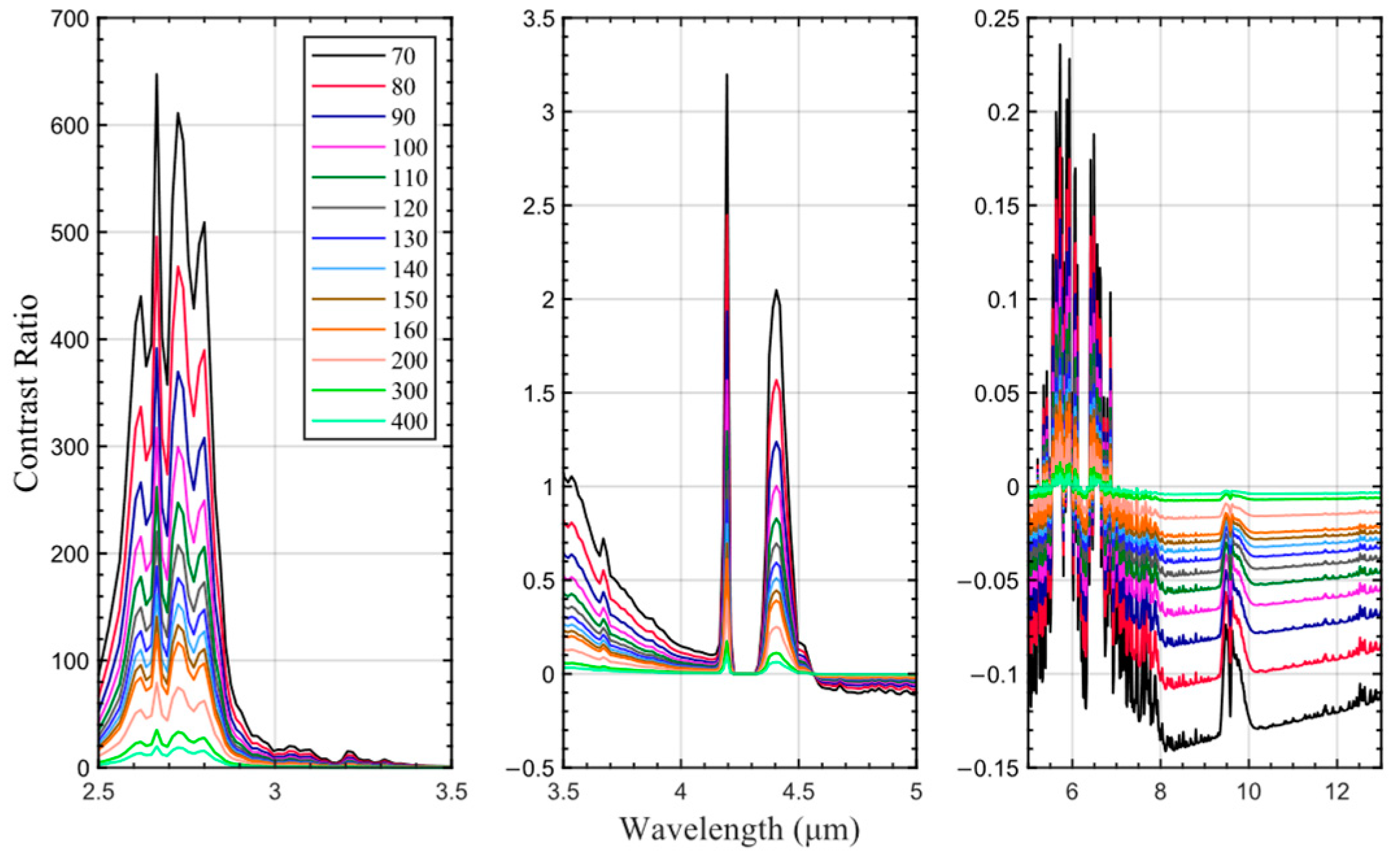
4.1. Space-Based Infrared Detection Spectral Window for Aircraft
4.2. The Challenge of Space-Based Infrared Detection of Aircraft
5. Conclusions
Author Contributions
Funding
Data Availability Statement
Acknowledgments
Conflicts of Interest
References
- Kasturi, E.; Devi, S.P.; Kiran, S.V.; Manivannan, S. Airline Route Profitability Analysis and Optimization Using BIG DATA Analyticson Aviation Data Sets under Heuristic Techniques. Procedia Comput. Sci. 2016, 87, 86–92. [Google Scholar] [CrossRef] [Green Version]
- Liu, Y.; Xu, B.; Zhi, W.; Hu, C.; Dong, Y.; Jin, S.; Lu, Y.; Chen, T.; Xu, W.; Liu, Y.; et al. Space Eye on Flying Aircraft: From Sentinel-2 MSI Parallax to Hybrid Computing. Remote Sens. Environ. 2020, 246, 111867. [Google Scholar] [CrossRef]
- Beier, K. Infrared Radiation Model for Aircraft and Reentry Vehicle. In Proceedings of the Infrared Technology XIV, San Diego, CA, USA, 15–18 August 1988; Spiro, I.J., Ed.; SPIE: Washington, DC, USA, 1988; Volume 0972, pp. 363–374. [Google Scholar]
- Iannarilli, F.J., Jr.; Wohlers, M.R. End-to-End Scenario-Generating Model for IRST Performance Analysis. In Proceedings of the Signal and Data Processing of Small Targets, Orlando, FL, USA, 1 April 1991; Drummond, O.E., Ed.; SPIE: Washington, DC, USA, 1991; Volume 1481, pp. 187–197. [Google Scholar]
- Bishop, G.J.; Caola, M.J.; Geatches, R.M.; Roberts, N.C. SIRUS Spectral Signature Analysis Code. In Proceedings of the Targets and Backgrounds IX: Characterization and Representation, Orlando, FL, USA, 21–25 April 2003; Watkins, W.R., Clement, D., Reynolds, W.R., Eds.; SPIE: Washington, DC, USA, 2003; Volume 5075, pp. 259–269. [Google Scholar]
- Johansson, M.; Dalenbring, M. SIGGE, A Prediction Tool for Aeronautical IR Signatures, and Its Applications. In Proceedings of the 9th AIAA/ASME Joint Thermophysics and Heat Transfer Conference, San Francisco, CA, USA, 5–8 June 2006; p. 3276. [Google Scholar]
- Cathala, T.; Douchin, N.; Joly, A.; Perzon, S. The Use of SE-WORKBENCH for Aircraft Infrared Signature, Taken into Account Body, Engine, and Plume Contributions. In Proceedings of the Infrared Imaging Systems: Design, Analysis, Modeling, and Testing XXI, Orlando, FL, USA, 5–9 April 2010; SPIE: Washington, DC, USA, 2010; Volume 7662, p. 76620U. [Google Scholar]
- Sonawane, H.R.; Mahulikar, S.P. Tactical Air Warfare: Generic Model for Aircraft Susceptibility to Infrared Guided Missiles. Aerosp. Sci. Technol. 2011, 15, 249–260. [Google Scholar] [CrossRef]
- Gangoli Rao, A. Infrared Signature Modeling and Analysis of Aircraft Plume. Int. J. Turbo Jet Engines 2011, 28, 187–197. [Google Scholar] [CrossRef]
- Mahulikar, S.P.; Rastogi, P.; Bhatt, A. Aircraft Signature Studies Using Infrared Cross Section and Infrared Solid Angle. J. Aircr. 2021, 59, 126–136. [Google Scholar] [CrossRef]
- Coiro, E.; Chatelard, C.; Durand, G.; Langlois, S.; Martinenq, J.-P. Experimental Validation of an Aircraft Infrared Signature Code for Commercial Airliners. In Proceedings of the 43rd AIAA Thermophysics Conference, New Orleans, LA, USA, 25–28 June 2012; p. 3190. [Google Scholar]
- Coiro, E. Global Illumination Technique for Aircraft Infrared Signature Calculations. J. Aircr. 2013, 50, 103–113. [Google Scholar] [CrossRef]
- Coiro, E.; Lefebvre, S.; Ceolato, R. Infrared Signature Prediction for Low Observable Air Vehicles. In Proceedings of the AVT-324 Specialists’ Meeting on Multi-Disciplinary Design Approaches and Performance Assessment of Future Combat Aircraft, NATO, Online, 28 September 2020. [Google Scholar]
- Yuan, H.; Wang, X.; Yuan, Y.; Li, K.; Zhang, C.; Zhao, Z. Space-Based Full Chain Multi-Spectral Imaging Features Accurate Prediction and Analysis for Aircraft Plume under Sea/Cloud Background. Opt. Express 2019, 27, 26027–26043. [Google Scholar] [CrossRef]
- Zhu, H.; Li, Y.; Hu, T.; Rao, P. An All-Attitude Motion Characterization and Parameter Analysis System for Aerial Targets. Infrared Laser Eng. 2018, 47, 168–173. [Google Scholar]
- Mahulikar, S.P.; Rao, G.A.; Kolhe, P.S. Infrared Signatures of Low-Flying Aircraft and Their Rear Fuselage Skin’s Emissivity Optimization. J. Aircr. 2006, 43, 226–232. [Google Scholar] [CrossRef]
- Mahulikar, S.; Potnuru, S.; Gangoli Rao, A. Study of Sunshine, Skyshine, and Earthshine for Aircraft Infrared Detection. J. Opt. Pure Appl. Opt. 2009, 11, 045703. [Google Scholar] [CrossRef]
- Mahulikar, S.; Vijay, S.; Potnuru, S.; Reddam, D.N.S. Aircraft Engine’s Lock-On Envelope Due to Internal and External Sources of Infrared Signature. Aerosp. Electron. Syst. IEEE Trans. 2012, 48, 1914–1923. [Google Scholar] [CrossRef]
- Baranwal, N.; Mahulikar, S.P. Infrared Signature of Aircraft Engine with Choked Converging Nozzle. J. Thermophys. Heat Transf. 2016, 30, 854–862. [Google Scholar] [CrossRef]
- Baranwal, N.; Mahulikar, S.P. IR Signature Study of Aircraft Engine for Variation in Nozzle Exit Area. Infrared Phys. Technol. 2016, 74, 21–27. [Google Scholar] [CrossRef]
- Zhang, J.; Qi, H.; Jiang, D.; Gao, B.; He, M.; Ren, Y.; Li, K. Integrated Infrared Radiation Characteristics of Aircraft Skin and the Exhaust Plume. Materials 2022, 15, 7726. [Google Scholar] [CrossRef] [PubMed]
- Huang, Y.; Cui, X. Modulation of Infrared Signatures Based on Anisotropic Emission Behavior of Aircraft Skin. Opt. Eng. 2015, 54, 123112. [Google Scholar] [CrossRef]
- Yuan, H.; Wang, X.-R.; Guo, B.-T.; Ren, D.; Zhang, W.-G.; Li, K. Performance Analysis of the Infrared Imaging System for Aircraft Plume Detection from Geostationary Orbit. Appl. Opt. 2019, 58, 1691–1698. [Google Scholar] [CrossRef] [PubMed]
- Zhu, H.; Li, Y.; Hu, T. Key Parameters Design of an Aerial Target Detection System on a Space-Based Platform. Opt. Eng. 2018, 57, 023107. [Google Scholar] [CrossRef]
- Yu, S.; Ni, X.; Li, X.; Hu, T.; Chen, F. Real-Time Dynamic Optimized Band Detection Method for Hypersonic Glide Vehicle. Infrared Phys. Technol. 2022, 121, 104020. [Google Scholar] [CrossRef]
- Zhou, X.; Ni, X.; Zhang, J.; Weng, D.; Hu, Z.; Chen, F. A Novel Detection Performance Modular Evaluation Metric of Space-Based Infrared System. Opt. Quantum Electron. 2022, 54, 274. [Google Scholar] [CrossRef]
- Ni, X.; Yu, S.; Su, X.; Chen, F. Detection Spectrum Optimization of Stealth Aircraft Targets from a Space-Based Infrared Platform. Opt. Quantum Electron. 2022, 54, 1–12. [Google Scholar] [CrossRef]
- Zhao, Y.; Dai, L.; Bai, S.; Liu, J.; Peng, H.; Wang, H. Design and implementation of full-spectrum spectral imager system. Spacecr. Recovery Remote Sens. 2018, 39, 38–50. (In Chinese) [Google Scholar]
- Qiu, X.; Zhao, H.; Jia, G.; Li, J. Atmosphere and Terrain Coupling Simulation Framework for High-Resolution Visible-Thermal Spectral Imaging over Heterogeneous Land Surface. Remote Sens. 2022, 14, 2043. [Google Scholar] [CrossRef]
- Shao, X.; Fan, H.; Lu, G.; Xu, J. An Improved Infrared Dim and Small Target Detection Algorithm Based on the Contrast Mechanism of Human Visual System. Infrared Phys. Technol. 2012, 55, 403–408. [Google Scholar] [CrossRef]
- Acharya, P.K.; Berk, A.; Anderson, G.P.; Anderson, G.P.; Larsen, N.F.; Tsay, S.C.; Stamnes, K.H. MODTRAN4: Multiple Scattering and Bidirectional Reflectance Distribution Function (BRDF) Upgrades to MODTRAN. In Proceedings of the Optical Spectroscopic Techniques and Instrumentation for Atmospheric and Space Research III, Denver, CO, USA, 18–23 July 1999; Larar, A.M., Ed.; SPIE: Washington, DC, USA, 1999; Volume 3756, pp. 354–362. [Google Scholar]
- Niu, Q.; Meng, X.; He, Z.; Dong, S. Infrared Optical Observability of an Earth Entry Orbital Test Vehicle Using Ground-Based Remote Sensors. Remote Sens. 2019, 11, 2404. [Google Scholar] [CrossRef] [Green Version]
- Niu, Q.; Yang, S.; He, Z.; Dong, S. Numerical Study of Infrared Radiation Characteristics of a Boost-Gliding Aircraft with Reaction Control Systems. Infrared Phys. Technol. 2018, 92, 417–428. [Google Scholar] [CrossRef]
- Ye, Q.; Sun, X.; Zhang, Y.; Zhang, C.; Shao, L.; Wang, Y. Modeling and Simulation of Infrared Radiation from Rocket Plume at Boosting Stage. In Proceedings of the International Symposium on Photoelectronic Detection and Imaging 2009: Advances in Infrared Imaging and Applications, Beijing, China, 24–26 May 2011; Volume 7383, pp. 355–362. [Google Scholar] [CrossRef]
- Zhou, G. Optimization of Radiation Model of Infrared Decoy with Neural Network. J. Phys. Conf. Ser. 2019, 1302, 042027. [Google Scholar] [CrossRef]
- Mahulikar, S.; Marathe, A.; Gangoli Rao, A.; Sane, S. Aircraft Plume Infrared Signature in Nonafterburning Mode. J. Thermophys. Heat Transf. 2005, 19, 413–415. [Google Scholar] [CrossRef]
- Modest, M.F. Radiative Heat Transfer; Academic Press: Cambridge, MA, USA, 2013. [Google Scholar]
- Rothman, L.S.; Gordon, I.E.; Barber, R.J.; Dothe, H.; Gamache, R.R.; Goldman, A.; Perevalov, V.I.; Tashkun, S.A.; Tennyson, J. HITEMP, the High-Temperature Molecular Spectroscopic Database. In Proceedings of the XVI Symposium on High Resolution Molecular Spectroscopy—HighRus-2009, Prague, Czech Republic, 3 September 2008; Volume 111, pp. 2139–2150. [Google Scholar] [CrossRef]
- Cota, S.A.; Kalman, L.S. Predicting Top-of-Atmosphere Radiance for Arbitrary Viewing Geometries from the Visible to Thermal Infrared. In Proceedings of the Remote Sensing System Engineering III, San Diego, CA, USA, 1–5 August 2010; Ardanuy, P.E., Puschell, J.J., Eds.; SPIE: Washington, DC, USA, 2010; Volume 7813, p. 781307. [Google Scholar]
- Guorui, J.; Huijie, Z.; Na, L. Simulation of Hyperspectral Scene with Full Adjacency Effect. In Proceedings of the IGARSS 2008-2008 IEEE International Geoscience and Remote Sensing Symposium, Boston, MA, USA, 7–11 July 2008; Volume 3, pp. III-724–III-727. [Google Scholar]
- Mouroulis, P.; Green, R.O. Spectral Response Evaluation and Computation for Pushbroom Imaging Spectrometers. In Proceedings of the Current Developments in Lens Design and Optical Engineering VIII, San Diego, CA, USA, 26–30 August 2007; Mouroulis, P.Z., Smith, W.J., Johnson, R.B., Eds.; SPIE: Washington, DC, USA, 2007; Volume 6667, p. 66670G. [Google Scholar]
- Zanoni, V.; Davis, B.; Ryan, R.; Gasser, G.; Blonski, S. Remote Sensing Requirements Development: A Simulation-Based Approach. In Proceedings of the The ISPRS Commission I Symposium, Denver, CO, USA, 9–12 July 2002. [Google Scholar]
- Merchant, C.J.; Embury, O.; Bulgin, C.E.; Block, T.; Corlett, G.K.; Fiedler, E.; Good, S.A.; Mittaz, J.; Rayner, N.A.; Berry, D.; et al. Satellite-Based Time-Series of Sea-Surface Temperature since 1981 for Climate Applications. Sci. Data 2019, 6, 223. [Google Scholar] [CrossRef] [Green Version]
- Meerdink, S.K.; Hook, S.J.; Roberts, D.A.; Abbott, E.A. The ECOSTRESS Spectral Library Version 1.0. Remote Sens. Environ. 2019, 230, 111196. [Google Scholar] [CrossRef]
- Li, N.; Lv, Z.; Wang, S.; Gong, G.; Ren, L. A Real-Time Infrared Radiation Imaging Simulation Method of Aircraft Skin with Aerodynamic Heating Effect. Infrared Phys. Technol. 2015, 71, 533–541. [Google Scholar] [CrossRef]
- EUMETSAT NWP SAF IR_SRF of GF5 VIMS. Available online: https://nwp-saf.eumetsat.int/downloads/rtcoef_rttov13/ir_srf/rtcoef_gf5_1_vims_srf.html (accessed on 8 August 2022).
- Mahulikar, S.P.; Sonawane, H.R.; Arvind Rao, G. Infrared Signature Studies of Aerospace Vehicles. Prog. Aerosp. Sci. 2007, 43, 218–245. [Google Scholar] [CrossRef]
- Abrams, M.; Hook, S.; Ramachandran, B. ASTER User Handbook. Available online: https://lpdaac.usgs.gov/documents/1319/ASTER_User_Handbook_v4.pdf (accessed on 31 August 2022).
- Luo, X.; Wu, Y.; Wang, F. Target Detection Method of UAV Aerial Imagery Based on Improved YOLOv5. Remote Sens. 2022, 14, 5063. [Google Scholar] [CrossRef]
- Yao, Y.; Wang, M.; Fan, G.; Liu, W.; Ma, Y.; Mei, X. Dictionary Learning-Cooperated Matrix Decomposition for Hyperspectral Target Detection. Remote Sens. 2022, 14, 4369. [Google Scholar] [CrossRef]
- Heiselberg, P.; Heiselberg, H. Aircraft Detection above Clouds by Sentinel-2 MSI Parallax. Remote Sens. 2021, 13, 3016. [Google Scholar] [CrossRef]
- Stair, A. MSX Design Parameters Driven by Targets and Backgrounds. Johns Hopkins Apl. Technol. Dig. 1996, 17, 11–18. [Google Scholar]
- Cawley, S.J. The Space Technology Research Vehicle 2 Medium Wave Infra Red Imager. Acta Astronautica 2003, 52, 717–726. [Google Scholar] [CrossRef]
- Li, B.; Xiao, C.; Wang, L.; Wang, Y.; Lin, Z.; Li, M.; An, W.; Guo, Y. Dense Nested Attention Network for Infrared Small Target Detection. IEEE Trans. Image Process. 2022, 14, 8. [Google Scholar] [CrossRef]


| Parameters | Values |
|---|---|
| Imaging time (UTC) | 25 June 2019 4:38:54 |
| View zenith (°) | 179.76 |
| View azimuth (°) | 164.25 |
| Band number | B7–B12 |
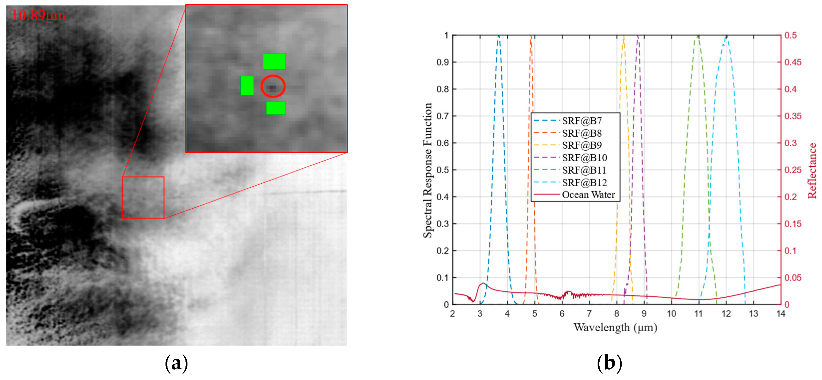
| Band range | B7:3.45–3.90μm B8:4.76–4.96μm B9:8.05–8.45μm B10:8.57–8.93μm B11:10.5–11.3μm B12:11.4–12.5μm |
| GSD (m) | 40 |
| NEΔT (K) | 0.15K@300K |
| MTF | 0.15 |
| Parameters | Values | Parameters | Values |
|---|---|---|---|
| Aircraft type | Boeing 777-246 | Wing area (m2) | 427.8 |
| Flight altitude (m) | 12,192 | Fuselage radius (m) | 3.1 |
| Flight speed (m/s) | 218.64 | Nozzle radius (m) | 0.57 |
| Fuselage Length (m) | 63.7 | Nozzle number | 2 |
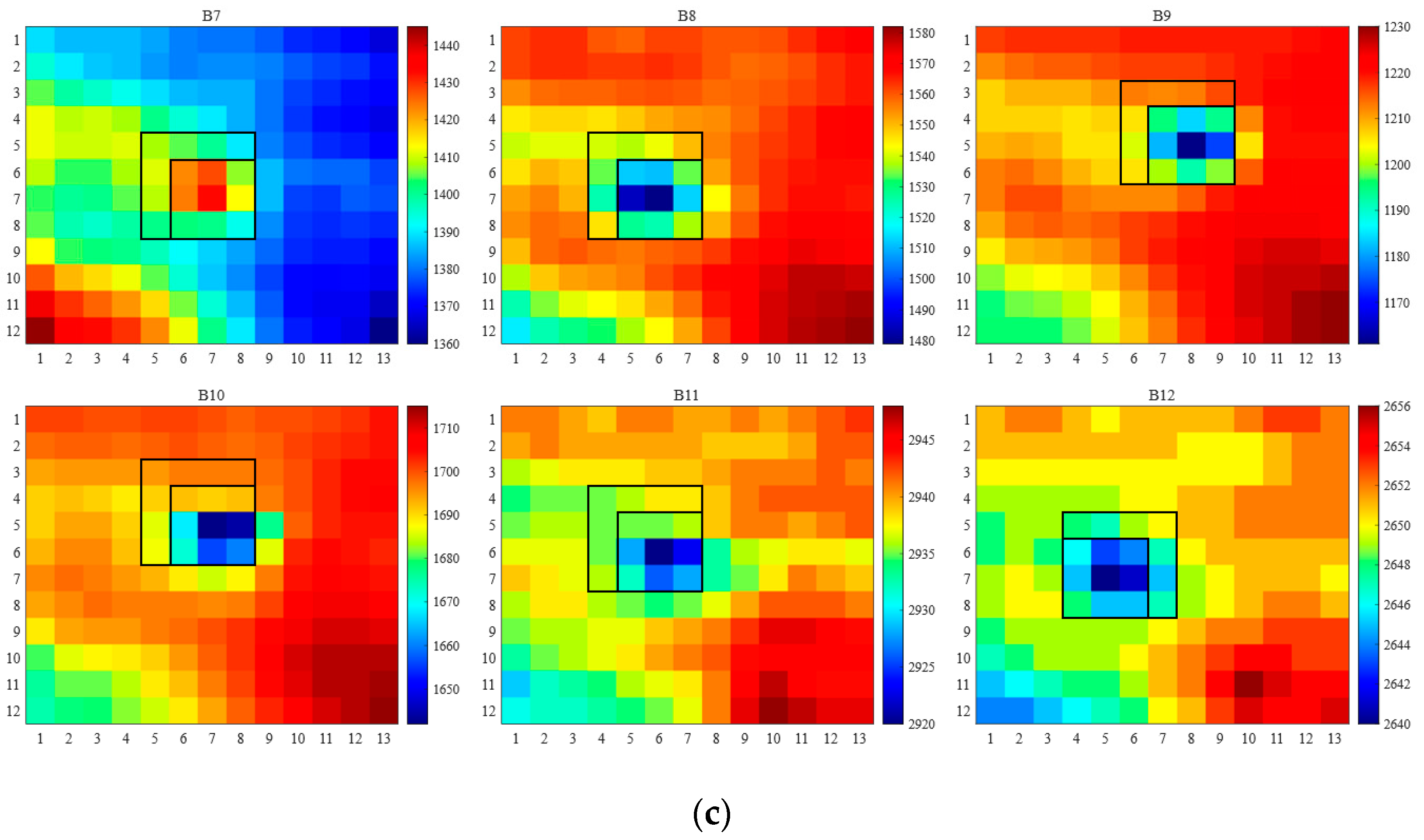
| Band | Aircraft 3 × 3 | Pure Aircraft 3 × 3 | T-B Contrast 3 × 3 | |||
| RE | AE | RE | AE | Onboard | Simulation | |
| B7 | −28.46% | −0.0810 | 161.95% | 0.8563 | 5.54% | 20.57% |
| B8 | 1.47% | 0.0161 | −20.64% | −0.1269 | −2.61% | −3.24% |
| B9 | 4.34% | 0.2804 | −69.48% | −2.7987 | −2.26% | −4.67% |
| B10 | 5.56% | 0.4152 | −73.91% | −4.0741 | −1.58% | −4.65% |
| B11 | 4.08% | 0.3218 | −60.80% | −3.1544 | −2.05% | −4.28% |
| B12 | −6.04% | −0.4017 | −40.55% | −1.471 | −2.71% | −4.08% |
| |MEAN| | 8.32% | 0.2527 | 71.22% | 2.0802 | 2.79% | 6.91% |
| Band | Aircraft 4 × 4 | Pure aircraft 4 × 4 | T-B contrast 4 × 4 | |||
| RE | AE | RE | AE | Onboard | Simulation | |
| B7 | −20.40% | −0.0573 | 123.92% | 0.7665 | 4.20% | 11.57% |
| B8 | 0.74% | 0.0081 | 5.98% | 0.0275 | −1.91% | −1.82% |
| B9 | 3.12% | 0.2039 | −67.18% | −2.5168 | −1.41% | −2.63% |
| B10 | 4.13% | 0.3106 | −72.90% | −3.8681 | −0.98% | −2.61% |
| B11 | 2.83% | 0.2248 | −55.15% | −2.5014 | 1.41% | −2.41% |
| B12 | −7.27% | −0.4871 | −15.10% | −0.3834 | 2.04% | −2.29% |
| |MEAN| | 6.42% | 0.2153 | 56.71% | 1.6773 | 1.99% | 3.89% |
Disclaimer/Publisher’s Note: The statements, opinions and data contained in all publications are solely those of the individual author(s) and contributor(s) and not of MDPI and/or the editor(s). MDPI and/or the editor(s) disclaim responsibility for any injury to people or property resulting from any ideas, methods, instructions or products referred to in the content. |
© 2023 by the authors. Licensee MDPI, Basel, Switzerland. This article is an open access article distributed under the terms and conditions of the Creative Commons Attribution (CC BY) license (https://creativecommons.org/licenses/by/4.0/).
Share and Cite
Li, J.; Zhao, H.; Gu, X.; Yang, L.; Bai, B.; Jia, G.; Li, Z. Analysis of Space-Based Observed Infrared Characteristics of Aircraft in the Air. Remote Sens. 2023, 15, 535. https://doi.org/10.3390/rs15020535
Li J, Zhao H, Gu X, Yang L, Bai B, Jia G, Li Z. Analysis of Space-Based Observed Infrared Characteristics of Aircraft in the Air. Remote Sensing. 2023; 15(2):535. https://doi.org/10.3390/rs15020535
Chicago/Turabian StyleLi, Jiyuan, Huijie Zhao, Xingfa Gu, Lifeng Yang, Bin Bai, Guorui Jia, and Zengren Li. 2023. "Analysis of Space-Based Observed Infrared Characteristics of Aircraft in the Air" Remote Sensing 15, no. 2: 535. https://doi.org/10.3390/rs15020535