Target Detection Method Based on Adaptive Step-Size SAMP Combining Off-Grid Correction for Coherent Frequency-Agile Radar

Abstract

Coherent frequency-agile radar (FAR) has a low probability of intercept (LPI) and excellent performance of electronic counter-countermeasures (ECCM) and electromagnetic compatibility, which can improve radar cooperation and survivability in complex electromagnetic environments. However, due to the nonlinearity of radar carrier frequency and the limitation of the Doppler tolerance of high-resolution range cells, the undesirable blind-speed sidelobes are generated in the two-dimensional (2D) range–velocity plane after coherent integration (CI) using the traditional methods based on a matching filter, which may degrade the target detection performance. To solve this problem, an adaptive step-size sparsity adaptive matching pursuit (SAMP) algorithm combining off-grid correction (ASSAMP-OC) is proposed in this paper, which seeks to achieve a better trade-off between recovery efficiency and detection performance. Firstly, an adaptive iteration step size based on the Spearman correlation coefficients (SCCS) is devised, which solves the problem of the traditional SAMP algorithm being insensitive to the change in iteration step size when the residuals vary slightly, and improves the recovery speed. Secondly, the off-grid correction method by combining a regularized stagewise backtracking idea and gradient descent optimization (GDO) is adopted to improve the recovery accuracy and suppress the blind-speed sidelobe energy (BSSE), which helps to reduce CI gain loss and improve the target detection performance without the prior information of the sparsity lever. Finally, simulation and experimental results demonstrate the effectiveness and efficiency of the proposed method in terms of target detection probability, target signal energy ratio after recovery, and computational cost, compared to several existing methods.

1. Introduction

The development of radar technology lies in the constant pursuit of better performance: longer radar range, higher range resolution, stronger target detection and recognition capabilities [1,2], etc. Due to the increasingly complex electromagnetic environment, on the other hand, radar survivability itself has become a key factor that must be considered in radar development [3,4]. How to improve electronic counter-countermeasures (ECCM) and radar detection performance by using new technologies has become an important topic. Modern jammers are optimized against coherent radars, in a way to achieve the effects of suppression, deception, and compound interference. In the face of complex interference, the most effective way for radar is to make the interference unable to predict the form of the radar-transmitted signal [5,6]. For example, the coherent frequency-agile radar (FAR) can quickly switch the carrier frequency of each pulse within the entire bandwidth range of the radar to counter the reconnaissance and intercept of radar signal parameters by jammers, which makes it difficult for jammers to implement accurate interference on the radar effectively. Besides the advantages of anti-interference, FAR can reduce the correlation between two consecutive pulses of clutter by transmitting frequency-agile signals, which contributes to suppressing the clutter and improving target detection, identification, and tracking performance. In summary, the coherent FAR has a high-resolution range and velocity space, as well as an excellent low probability of intercept (LPI), anti-interference performance, and electromagnetic compatibility, which can improve the cooperation and survival ability of the radar in a complex electromagnetic environment. Moreover, with the development of the technology of coherent frequency synthesizers, coherent FAR has been widely applied. Therefore, it is important to investigate the signal-processing algorithms of coherent FAR [7,8].

To improve the clutter suppression and target detection performance for coherent FAR, the coherent integration (CI) method is necessary. However, if the radiant source radar transmits the carrier frequency-agile signal, it will destroy the phase consistency of different echoes, which may reduce the CI gain, bringing huge challenges to target detection. Conventional CI methods, such as Keystone transform (KT) [9], adjacent cross-correlation function (ACCF) [10], axis rotation moving target detection (MTD) [11], etc., can only be applied to traditional radar signal processing. In the past few years, some scholars have already carried out many studies on the CI algorithms of FAR. For instance, stretch processing including a bank of Doppler filters in [12,13] is exploited to design the two-dimensional (2D) high-resolution range–velocity-matched filters. It is based on the principle of matched filtering, with the advantage that the whole calculation process is a linear operation, the calculation complexity is low, and the result is relatively stable. However, due to the fact that the carrier frequency of FAR changes irregularly, it has a problem with high blind-speed sidelobe energy (BSSE) in the 2D range–velocity plane after CI processing, which may lead to an increase in false alarm rate and weak target miss detection rate. To suppress the BSSE and enhance the detection performance, a method by pre-designing the carrier frequency sequences is proposed [14]. However, according to Parseval’s theorem, the amplitude of the highest sidelobe in the range profile generated by discrete Fourier transform should be at least greater $1/\sqrt{M}$ than that of the mainlobes, where $M$ is the number of pulses. In addition, the pre-designing carrier frequency sequence method does not consider the situation where there are multiple targets in the observation scene, and it cannot guarantee that the BSSE of multiple targets will remain at a low level after superimposing each other. Therefore, as for the matching filter method, it is limited to suppressing the BSSE by carefully selecting the agile mode for FARs. Another method, such as the radon-Fourier transform (RFT), is proposed. Its CI results are obtained by compensating the phase fluctuation according to the target motion information using the method of a 2D range–velocity search, and the BSSE can be effectively suppressed. However, this algorithm has a higher computational burden. In order to address this problem, in [15], frequency bin RFT and sub-band RFT methods for the fast implementation of RFT based on fast Chirp-Z transform are proposed. In [16], an improved RFT optimized by the particle swarm optimization (PSO) algorithm is exploited. In [17], a sub-aperture adaptive RFT method is proposed for fast weak target detection. However, those methods generally demand complex pre-processing, such as sub-band searching [15], suitable multiparameter initialization [16], and sub-aperture division [17]. In [18], a whale optimization algorithm-based RFT (WOA-RFT) for efficient CI without complex pre-processing is proposed. However, the computational cost indicates that it may still be difficult to satisfy the requirement of real-time detection.

In recent years, sparse representation has made great progress in radar detection, radar 3D imaging, and other fields, and also provides many new ideas for coherent FAR signal processing [19,20,21,22,23]. The sparse recovery algorithm is an important part of sparse representation and significantly influences the sparse representation results [24,25]. Existing recovery algorithms can be summarized into two classes: the convex optimization method and the matching pursuit (MP) method [26,27]. The computational complexity of the convex optimization method is high, such as the basis pursuit (BP) algorithm [28], which is not incommensurate with practical large-scale applications [29]. Based on the iterative greedy pursuit, the MP method can achieve sparse recovery [30] with lower computational complexity. Typical ones include the orthogonal matching pursuit (OMP) [31], the compressive sampling MP (CoSaMP) [32], and regularized OMP (ROMP) algorithms [33]. Specifically, the OMP is presented to optimize the traditional MP by orthogonalizing the atoms of the support set. The CoSaMP algorithm selects multiple atoms per iteration, which is developed from the OMP. Both of them are proposed based on the idea of backtracking; the significant difference between the two algorithms is that atoms of the ROMP already selected in each iteration are always retained, while atoms of the CoSaMP selected in each iteration may be discarded in the next iteration. Although the recovery complexity of those methods, close to O (KMN), is much less than that of the BP methods, those greedy algorithms require the prior sparsity lever of the target signal, which might not be accessible in practical applications [34].

Sparsity adaptive matching pursuit (SAMP) can reconstruct the target signal without the limitation of the sparsity lever [35,36]. However, the iteration step size of the SAMP algorithm is difficult to determine in practice and is not adaptive, which may seriously influence the recovery performance of the target signal. For example, if the iteration step size of the SAMP is large, overestimation will occur, which reduces the recovery accuracy. Otherwise, more iterations will be required, which reduces the recovery efficiency. In [37], several improved SAMP algorithms are developed, such as the reducing iteration OMP (RIOMP) [38], which combines the idea of backtracking to set up a threshold to reduce the number of iterations; the variable step-size SAMP (VSSAMP) [39], which devises the binary variable step sizes based on energy residual theory; the adaptive step-size matching pursuit (AStMP) [40,41], which can accurately estimate sparsity with the adaptive step size at each iteration; and the correlation coefficient SAMP (CCSAMP) [34], which can accelerate the conventional SAMP during each iteration without comparing the current iteration results to that of the previous iteration with varying iteration step sizes. The RIOMP and the AStMP algorithms can effectively improve the accuracy of the sparse recovery algorithm, but the number of iterations is still high. The VSSAMP algorithm devises an adaptive step size, but the step size may not be adjusted in time when the iteration residuals do not change significantly. Although the CCSAMP can address the insensitivity of the step size to the iteration residuals, the nonstationary blind-speed sidelobes may be generated due to the off-grid problems, which may result in significant degradation of target detection performance, especially in low-signal-to-clutter-ratio (SCR) environments.

The major shortcomings of the aforementioned SAMP algorithms include the high BSSE and computational costs. Aiming at these problems, an adaptive step-size SAMP algorithm combining off-grid correction (ASSAMP-OC) is proposed in this paper. The proposed algorithm mainly consists of two key steps: adaptive step size design and off-grid correction, the framework is shown in Figure 1. Moreover, the main contributions of this paper can be summarized as follows:

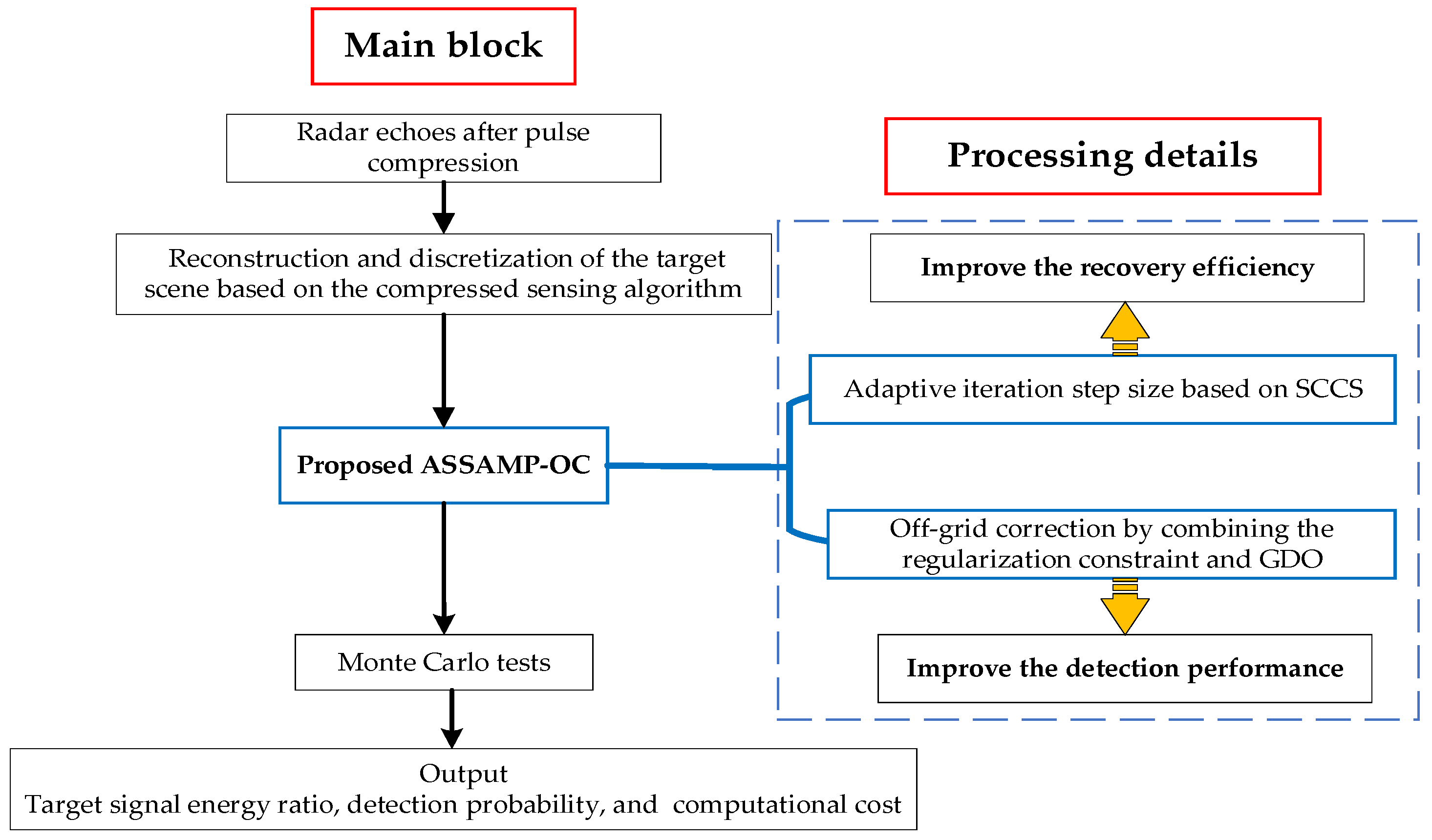
• Improving the signal recovery efficiency: An adaptive step-size method based on Spearman correlation coefficients (SCCS) is proposed to solve the problem of a large number of iterations in the traditional SAMP method. In addition, a convergence criterion based on polynomial fitting error is introduced, which is beneficial to further speed up the algorithm.
• Improving the target detection performance: The BSSE can be suppressed effectively by using off-grid correction by combining the regularization theory and gradient descent optimization (GDO), which can improve the signal recovery quality and reduce the CI gain loss without the prior information of the sparse lever.

The remaining sections of this paper are organized as follows. In Section 2, the echo signal model of FAR is presented and the target scene via a compressed sensing (CS) algorithm is reconstructed. In Section 3, the traditional SAMP is introduced, and then the ASSAMP-OC is proposed. Section 4 discusses the simulation and experimental results of the proposed ASSAMP-OC, ROMP, SAMP, CCSAMP, SAMP based on the off-grid correction (SAMP-OC), and WOA-RFT. Finally, Section 5 summarizes the conclusion.

2. Echo Signal Model and Sparse Representation

Suppose that the FAR transmits a linear frequency-modulated (LFM) signal, and the carrier frequencies of pulse trains are varied with a random frequency step. The transmitted signal of radar is expressed as:

$$s_m(t_{\mathit{f}})=\mathrm{rect}(\frac{t_{\mathit{f}}}{T_p})\exp (j2\pi {\mathit{f}}_m{t}_{\mathit{f}})\exp (j\pi {\mathit{f}}_{m}k{t}_{\mathit{f}}^2)$$

(1)

where $\mathrm{rect}(\frac{t_{\mathit{f}}}{T_p})=\left\{\begin{array}{l}1,\begin{array}{cc}& t_{\mathit{f}}\le \left|\frac{T_p}{2}\right|\end{array}\\ 0,\begin{array}{cc}& \mathrm{others}\end{array}\end{array}\right.$; $t_{\mathit{f}}$ is the fast time; $T_p$ is the pulse width; ${\mathit{f}}_m={\mathit{f}}_0+d_m\Delta \mathit{f}$ ($m=0,1,2,\dots ,M-1$) represents Random frequency, where ${\mathit{f}}_0$ is the radar carrier frequency; $d_m$ is a random integer between 0 and the floor integer $⌊B/\Delta \mathit{f}⌋$; $B$ is the synthetic bandwidth of the radar baseband; $\Delta \mathit{f}$ is the frequency step size; $m$ is the pulse number; $M$ is the total pulse number during coherent integration interval (CPI); $k$ is the frequency modulation slope.

As for the range spread target, the target signal received by the radar can be viewed as a linear superposition of the echoes of all the target scatterers with the same motion speeds in the observation scene. For simplicity, suppose that the number of target scatterers is set to 1, then the received signal after down-conversion and pulse compression (PC) can be formed as:

$$s_{\mathit{r}}{}_m(t_{\mathit{f}})=A_0\mathrm{rect}(\frac{t_{\mathit{f}}-\tau }{T_p})\sin c(k{T}_p(t_{\mathit{f}}-\tau ))\exp (-j2\pi {\mathit{f}}_m{t}_{\mathit{f}})$$

(2)

where $A_0$ denotes the amplitude of target reflectivity; $\sin c\left(\mathit{x}\right)=\sin \pi \mathit{x}/(\pi \mathit{x})$ denotes the sinc function. Suppose the target is moving radially at a constant speed: $\tau =2R(t_m)/c$ denotes the time delay; $R(t_m)=R_0+v_{0}m{T}_{\mathit{r}}$ denotes the range between radar and target; $t_m$ is the slow time; $c$ is the light speed. $R_0$ and $v_0$ denote the target radial range and velocity at the initial time, respectively; $T_{\mathit{r}}$ is the pulse repetition interval (PRI).

The echo signal on the range cell where the target is located is extracted along the slow time dimension as follows:

$$\mathit{y}(m)=A_0\exp \left(-j4\pi ({\mathit{f}}_0+d_m\Delta \mathit{f})\frac{R(t_m)}{c}\right)\exp \left(-j4\pi {\mathit{f}}_0\frac{v_{0}m{T}_{\mathit{r}}}{c}\left(1+\frac{d_m\Delta \mathit{f}}{{\mathit{f}}_0}\right)\right)$$

(3)

From Equation (3), it can be seen that as the number of pulses $m$ increases, the phase of the slow time dimension sampled signal changes unevenly, and the high blind-speed sidelobes may be generated in the 2D range–velocity plane after CI, which may lead to the degradation of the detection performance, or even the detection failure. Therefore, the traditional matched filtering-based CI method is no longer applicable.

To address this problem, we discretize target echoes of Equation (3) in the 2D range–Doppler plane. Specifically, the possible range and velocity values of the target are discretized into $\mathit{P}$ and $Q$ grid points, respectively. Equation (3) can be rewritten as follows:

$$\mathit{y}(m)={\displaystyle \sum _{p\in {\Omega }_p}{\displaystyle \sum _{q\in {\Omega }_q}\alpha (p,q)\exp \left(jp{d}_m\right)\exp (jqm{\eta }_m)}}$$

(4)

where ${\Omega }_p$ and ${\Omega }_q$ represent all possible range and velocity sets of the target, respectively. ${\eta }_m=\left(1+\frac{d_m\Delta \mathit{f}}{{\mathit{f}}_0}\right)$, $\alpha (p,q)$ indicates the scattering coefficient of the target corresponding to a grid point $(p,q)$ in the 2D range–Doppler plane, where $p=-4\pi \Delta \mathit{f}\frac{R}{c}$ and $q=-\frac{4\pi {\mathit{f}}_{0}v{T}_{\mathit{r}}}{c}$ represent the high-resolution range phase factor and velocity phase factor, respectively.

The main task of radar signal processing lies in the construction of the target scene, such as the estimation of the echo scattering coefficient $\alpha (p,q)$ in a 2D high-resolution range–Doppler plane according to the received echoes in Equation (4). Additionally, the grids should include all of the high-resolution range–velocity cells of interest, and the quantity of grids determines how precise the constructed scene is. In particular, the grid becomes denser as the required precision increases. However, practical application constraints arise because the radar system imposes a limit on the range–velocity resolution, preventing an unlimited increase in the number of grids.

After discretization, the echo scattering coefficient $\alpha (p,q)$ of the scene can be represented by a complex matrix $\Gamma$ of dimensions $\mathit{P}\times Q$ as follows:

$$\Gamma =\left[\begin{array}{ccc}a(p_0,q_0)& \cdots & a(p_0,q_{Q-1})\\ \cdots & \ddots & \cdots \\ a(p_{\mathit{P}-1},q_0)& \cdots & a(p_{\mathit{P}-1},q_{Q-1})\end{array}\right]$$

(5)

where $(p_l,q_l)$ denotes range–velocity pairs, $l=0,1,2,\dots ,\mathit{P}Q-1$.

Vectorize the columns of the matrix $\Gamma$ and then form the vector $\mathit{x}$ written as follows:

$$\mathit{x}={\left[a(p_0,q_0),\dots ,a(p_{\mathit{P}-1},q_{Q-1}),\dots ,a(p_{\mathit{P}-1},q_0),\dots ,a(p_{\mathit{P}-1},q_{Q-1})\right]}^{\mathrm{T}}$$

(6)

Assuming that the range–velocity pairs corresponding to the $l\mathrm{th}$ element of the vector $\mathit{x}\in {\mathrm{C}}^{\mathit{P}Q}$ are $(p_{l_p},q_{l_q})$, $l_p=0,1,\dots ,\mathit{P}-1, l_q=0,1,2,\dots ,Q-1$. Consequently, Equation (4) can be written as:

$$\mathit{y}(m)={\displaystyle \sum _{l_p=0}^{\mathit{P}-1}{\displaystyle \sum _{l_q=0}^{Q-1}{\mathit{x}}_l{e}^{j{p}_{l_p}{d}_m+j{q}_{l_q}m{\eta }_m}}}$$

(7)

Then, from Equation (7), the echo signals during CPI can be written in matrix form as follows:

$$\mathit{y}=\mathbf{\Phi }\mathit{x}$$

(8)

where $\mathit{y}={[\mathit{y}(0),\mathit{y}(1),\dots ,\mathit{y}(M-1)]}^T\in {\mathrm{C}}^M$ is the detected signal; $\mathbf{\Phi }=[\varphi (0),\varphi (1),\dots ,{\varphi }_{\mathit{P}Q-1}]\in {\mathrm{C}}^{M\times \mathit{P}Q}$ is the sensing matrix.

The recovery of the observed scene can be modeled to estimate the vector $\mathit{x}$ in Equation (8). The zero elements in the vector $\mathit{x}$ mean that there are no obvious target scatterers on the corresponding high-resolution range and velocity cells. Based on the location of the nonzero elements in the vector $\mathit{x}$, the information on the high-resolution range and velocity of the target can be obtained. Generally, we regard Equation (8) as a sparse representation of the echo signal based on CS theory. The traditional SAMP can achieve signal recovery results when the sensing matrix $\mathbf{\Phi }$ satisfies the restricted isometry property (RIP) [42] without the prior information of the sparse level.

3. Proposed Method

3.1. Analysis of the SAMP Algorithm

To better describe the SAMP algorithm, we define iteration step size $s$, iteration residual ${\mathit{r}}_t$, candidate set $C_t$, and support set $F_t$, where $t$ is the number of iterations. The conceptual diagram of the SAMP algorithm is shown in Figure 2.

The initialization of the SAMP algorithm can be expressed as:

$$\left\{\begin{array}{l}{\mathit{r}}_0=\mathit{y}\\ F_0=\varnothing \\ L=s_0\\ t=1\end{array}\right.$$

(9)

where $L$ is the index set size. The $L$ biggest values in $u$ are chosen; the associated set of sequence numbers is specified as $J_t$. $u$ can be expressed as:

$$u=‖{\mathbf{\Phi }}_{C_t}^{\mathrm{T}}{\mathit{r}}_{t-1}‖$$

(10)

where $‖.‖$ denotes the modal value of the vector; the set of columns of the sensing matrix $\mathbf{\Phi }$ selected by the candidate set $C_t$ is denoted by ${\mathbf{\Phi }}_{C_t}$; ${\mathit{r}}_{t-1}$ represents the residual at the $(t-1)\mathrm{th}$ iteration.

The support set $F_{t-1}$ of the previous iteration is chosen and merged with $J_t$ to construct the candidate set $C_t$ at the $t\mathrm{th}$ iteration; then, we can obtain the candidate set $C_t=F_{t-1}\cup J_t$. Let the vector ${\mathit{x}}_t$ denote the sparsity coefficient at the $t\mathrm{th}$ iteration, which can be obtained by using the least squares (LS) method as follows:

$${\mathit{x}}_t={({\mathbf{\Phi }}_{C_t}^{\mathrm{T}}{\mathbf{\Phi }}_{C_t})}^{-1}{\mathbf{\Phi }}_{C_t}^{\mathrm{T}}\mathit{y}$$

(11)

The $L\mathrm{th}$ atom with the largest absolute value from the vector ${\mathit{x}}_t$ is selected and labeled as ${\mathit{x}}_{tL}$, while the $L\mathrm{th}$ column corresponding to ${\mathbf{\Phi }}_{C_t}$ is selected and represented by ${\mathbf{\Phi }}_{F_t}$; the set of sequence numbers of ${\mathbf{\Phi }}_{F_t}$ remains in the support set $F_t=\mathrm{Max}(\left|{\mathit{x}}_t\mathit{y}\right|,L)$. Then, the residual at the $t\mathrm{th}$ iteration can be calculated as follows:

$${\mathit{r}}_t=\mathit{y}-{\mathbf{\Phi }}_{F_t}{({\mathbf{\Phi }}_{F_t}^{\mathrm{T}}{\mathbf{\Phi }}_{F_t})}^{-1}{\mathbf{\Phi }}_{F_t}^{\mathrm{T}}\mathit{y}$$

(12)

In the SAMP algorithm, if ${‖{\mathit{r}}_t‖}_2\ge {‖{\mathit{r}}_{t-1}‖}_2$, update the index set size $L=L+s$, and reform it into the SAMP algorithm for the next iteration; If $‖{\mathit{r}}_t‖\le ‖{\mathit{r}}_{end}‖$ or $t>T_{ma\mathit{x}}$, then the algorithm ends the iteration operation, and outputs the reconstructed sparsity coefficient ${\mathit{x}}_t$, where ${\mathit{r}}_{end}$ is the threshold of terminating iterations, which is close to zero, and $T_{\max }$ is the maximum number of iterations.

As for the SAMP algorithm, the vectors ${\mathit{y}}_t$ and ${\mathit{y}}_{tL}$ at the $t\mathrm{th}$ iteration can be obtained as follows:

$$\left\{\begin{array}{l}{\mathit{y}}_t={\mathbf{\Phi }}_{C_t}\mathit{x}={\mathbf{\Phi }}_{C_t}{({\mathbf{\Phi }}_{{}_{C_t}}^{\mathrm{T}}{\mathbf{\Phi }}_{{}_{C_t}})}^{-1}{\mathbf{\Phi }}_{{}_{C_t}}^{\mathrm{T}}\mathit{y}\\ {\mathit{y}}_{tL}=\mathit{y}-{\mathit{r}}_t={\mathbf{\Phi }}_{F_t}{({\mathbf{\Phi }}_{F_t}^{\mathrm{T}}{\mathbf{\Phi }}_{F_t})}^{-1}{\mathbf{\Phi }}_{F_t}^{\mathrm{T}}\mathit{y}\end{array}\right.$$

(13)

where the vectors ${\mathit{y}}_t$ and ${\mathit{y}}_{tL}$ are obtained based on the candidate set $C_t$ and the supporting candidate set $F_t$ ($F_t\subseteq C_t$). The relationship of vectors ${\mathit{y}}_t$ and ${\mathit{y}}_{tL}$ can be obtained as follows [34]:

$${\mathit{y}}_t={\mathbf{\Phi }}_{F_t}{({\mathbf{\Phi }}_{{}_{F_t}}^T{\mathbf{\Phi }}_{{}_{F_t}})}^{-1}{\mathbf{\Phi }}_{{}_{F_t}}^T\mathit{y}+{\mathit{r}}_{\mathit{r}t}={\mathit{y}}_{tL}+{\mathit{r}}_{\mathit{r}t}$$

(14)

According to Equation (14), the vectors ${\mathit{y}}_t$ and ${\mathit{y}}_{tL}$ are linearly correlated. Combined with Equation (12), the relationship between ${\mathit{r}}_{\mathit{r}t}$ and ${\mathit{r}}_t$ can be expressed as:

$$\left\{\begin{array}{l}{\mathit{r}}_{\mathit{r}t}={\mathit{r}}_t+{\mathit{y}}_t-\mathit{y}\\ ‖{\mathit{r}}_{\mathit{r}t}‖\le ‖{\mathit{r}}_t‖+‖{\mathit{y}}_t-\mathit{y}‖\end{array}\right.$$

(15)

According to Equation (15), the vectors ${\mathit{r}}_{\mathit{r}t}$ and ${\mathit{r}}_t$ decrease with iteration and approach a zero vector. Consequently, the reconstructed sparsity coefficient ${\mathit{x}}_t$ can be obtained, and the original signals can be recovered.

Based on the analysis above, although the SAMP algorithm does not require prior information of the sparsity level to recover the original signal, an iteration step size $s$ during algorithm operation is fixed, and is insensitive to the signal changes between two iterations with approximate residuals. In this case, the iteration step size $s$ of the SAMP may remain unchanged during several iterations, which may influence recovery efficiency. Specifically, the iteration number will be small, and the recovery efficiency will be improved when the iteration step size $s$ is large, but the recovery accuracy of the original signal may be reduced; the recovery accuracy of the original signal may be improved when the iteration step size $s$ is small, but the iteration number may be increased, which increases the computational complexity. Therefore, it is important to design an adaptive iteration step for signal recovery in real-world applications.

In addition, the problem of off-grids is generally present in many areas where CS algorithms are applied. As long as the estimated parameters are defined on a continuous space, the off-grid phenomenon is often unavoidable because it is impossible to know in advance the true parameters of the target to construct the grids correspondingly. For example, if the target scatterers are not located in the pre-discrete grid position after the range–velocity parameter space of the target is evenly divided into several grids, the off-grid problem will occur, resulting in a model mismatch between the predetermined sensing matrix and the target parameters, and the predetermined observation matrix cannot accurately estimate the true parameters of the target, as shown in Figure 3. In this case, the SAMP’s capability of signal recovery may be degraded, and the BSSE increases after CI processing, which leads to an increase in weak target missed detection rates, reducing the detection performance. To solve this problem, a straightforward idea is to make the grids denser, named overall and partial grid refinement methods, which will reduce the error between the real parameters of the target and the grids, as shown in Figure 4. However, since it is impossible to know in advance the true parameters of the target to construct the grids correspondingly, no matter how dense the parametric grids are, model mismatch may still occur; on the other hand, if the grids are too dense, it may lead to a stronger correlation between the columns of the sensing matrix, which significantly influences the performance of the CS-based recovery algorithm.

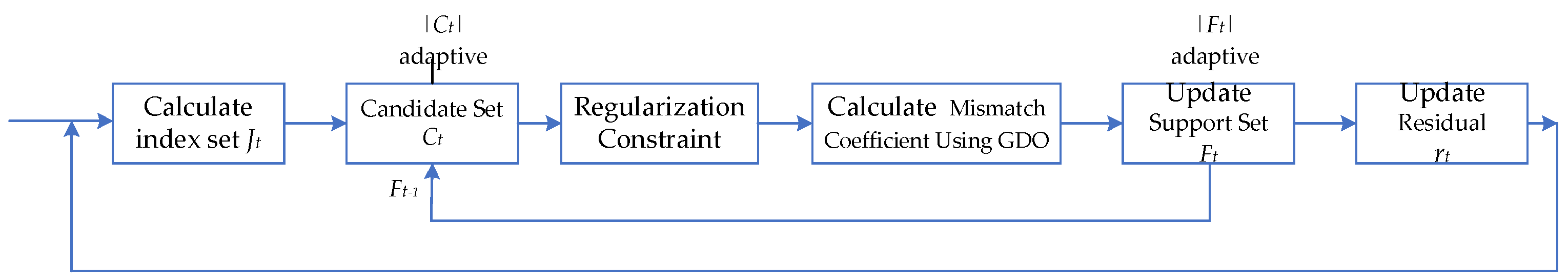
3.2. Analysis of the ASSAMP-OC Algorithm

Motivated by the disadvantages of the traditional SAMP algorithm, we propose a novel greedy algorithm, named ASSAMP-OC. The proposed method can effectively suppress the BSSE and improve detection performance without prior knowledge of the sparsity level, and the computational cost is low, which can bring an optional and efficient prospect for radar target detection under low-SCR circumstances. The proposed method mainly consists of two stages: adaptive step size design based on the SCCS and off-grid correction.

3.2.1. Adaptive Step Size Design

According to Equation (15), $‖{\mathit{r}}_t‖$ and $‖{\mathit{y}}_t-\mathit{y}‖$ gradually converge to zero as the iteration number $t$ increases, and the vector ${\mathit{r}}_{\mathit{r}t}$ tends to a zero vector. Combined with Equation (14), the vectors ${\mathit{y}}_t$ and ${\mathit{y}}_{tL}$ are linearly correlated and the vector ${\mathit{y}}_{tL}$ gradually tends to the vector ${\mathit{y}}_t$. Therefore, the recovery effect of the signal can be obtained by using the correlation coefficient between the vectors ${\mathit{y}}_t$ and ${\mathit{y}}_{tL}$. The correlation coefficient between the vectors ${\mathit{y}}_t$ and ${\mathit{y}}_{tL}$ changes with each iteration, thus it can be used to transform the iteration step size $s$, which can overcome the insensitivity problem of the iteration step size $s$ to the signal changes of the two iterations with similar residuals. In this paper, the similarity between the vectors ${\mathit{y}}_t$ and ${\mathit{y}}_{tL}$ is evaluated with the SCCS, which can be expressed as follows:

$${\rho }_t=\mathrm{SCCS}({\mathit{y}}_t,{\mathit{y}}_{tL})$$

(16)

Note that the detected signal may contain noise and clutter, which does not always satisfy the normal distribution characteristic in practical applications. Therefore, the function to determine the correlation coefficients of the vectors ${\mathit{y}}_t$ and ${\mathit{y}}_{tL}$ is used based on SCCS in this paper, instead of Pearson correlation coefficients (PCCS).

In addition, ${‖{\mathit{r}}_t‖}_2<{‖{\mathit{r}}_{t-1}‖}_2$ means that the estimated sparsity lever can better approach that of the original signal. In this case, for the SAMP algorithm, the index set size $L$ may remain for the next several iterations, which increases the iteration counter and reduces the recovery efficiency. To address this problem, the convergence criterion based on polynomial fitting errors is introduced to update the index set size $L$, which can further accelerate the signal recovery. The convergence criterion can be expressed as follows:

$$\left\{\begin{array}{l}L=L+s, \mathrm{if} {‖{\mathit{r}}_t‖}_2<{‖{\mathit{r}}_{t-1}‖}_2\mathrm{and}\left|‖{\mathit{r}}_t^{’}‖-‖{\mathit{r}}_t‖\right|\le {\varsigma }_1\\ L=L,\hspace{1em} \mathrm{if} {‖{\mathit{r}}_t‖}_2<{‖{\mathit{r}}_{t-1}‖}_2\mathrm{and}\left|‖{\mathit{r}}_t^{’}‖-‖{\mathit{r}}_t‖\right|>{\varsigma }_1\end{array}\right.$$

(17)

where ${\mathit{r}}_t^{’}$ is the fitting result of iteration residual ${\mathit{r}}_t$, which is obtained by performing the polynomial curve fitting method based on the vector $R_t=[{\mathit{r}}_0,{\mathit{r}}_1,\dots ,{\mathit{r}}_{t-1}]$. ${\varsigma }_1$ is the convergence threshold, which can be used to adjust the index set size $L$. It is noted that when the condition ${‖{\mathit{r}}_t‖}_2<{‖{\mathit{r}}_{t-1}‖}_2$ and $\left|‖{\mathit{r}}_t^{’}‖-‖{\mathit{r}}_t‖\right|>{\varsigma }_1$ is satisfied, it indicates that the estimated sparsity lever of the signal is gradually close to the real one, but the recovery accuracy does not yet satisfy our acceptable value, then we need to adjust $L=L+s$ (the estimated sparsity lever) to realize the approximate approach of the real sparsity level, which may further enhance the recovery efficiency.

3.2.2. Off-Grid Correction

Although the OMP method can realize high-accuracy recovery of echo signals, it needs the a priori information of the sparsity level. The traditional SAMP method can realize the recovery of echo signals in the absence of a priori information of sparsity level. However, it cannot solve the off-grid problem; the recovery performance is dramatically reduced, especially in a low SCR environment. To overcome this problem, in this paper, the off-grid correction method by combining the regularized atomic selection strategy and the GDO is used to improve the recovery accuracy. The off-grid correction method contributes to integrating the target signal energy and suppressing the BSSE after CI processing, which can reduce loss of the CI gain and improve the target detection performance. The proposed correction method mainly includes two stages: regularizing signals and calculating the mismatch coefficient using the GDO. The diagram of the off-grid correction process is presented in Figure 5.

• Regularized Constraint

The regularized idea to select the elements to update the candidate list is utilized at each stage with the estimated sparsity level, which can assure that the selected elements have maximum energy compared to those that are not selected. The regularized idea can be expressed as:

$$\left|S_t(i)\right|\le 2‖S_t(j)‖\begin{array}{cc}& \mathrm{for} \mathrm{all} i,j\in J_0\end{array}$$

(18)

where $[S_t,J_t]=\mathrm{supp}(\left|{\mathbf{\Phi }}^{\mathrm{T}}{\mathit{r}}_{t-1}\right|,L)=\mathrm{supp}(\left|u\right|,L)$.

According to the Formula (18), the purpose of the regularization processing is to choose $J_0\in J$ with the maximal average energy. As a consequence, the probability of the elements that possess less significance will be reduced, the recovery accuracy can be improved, and the computation complexity can also be reduced. In addition, a set $J$ is obtained from the $L$ biggest nonzero coordinates in magnitude of the observation vector $u$, or all of its nonzero coordinates, whichever set is smaller. Then, we continue to iterate and update the support set $F_t$ and the current residual ${\mathit{r}}_t$ as follows:

$$\left\{\begin{array}{l}[V_t,F_t]=\mathrm{supp}({\mathit{x}}_t,L)\\ {\mathit{r}}_t=\mathit{y}-{\mathbf{\Phi }}_{F_t}{\mathit{x}}_t\end{array}\right.$$

(19)

where ${\mathbf{\Phi }}_{F_t}$ represents the sensing matrix corresponding to the support set $F_t$.

• Acquisition of Mismatch Coefficient

Although the regularized processing contributes to improving the recovery accuracy, the off-grid problem is still present when target parameters lie off the selected grids in practical detection scenarios, and the recovery performance may degrade. To address the problem, the grid mismatch coefficient is calculated via the GDO method to adjust the sensing matrix to reduce the offset of the real position of the target scatterers from the discrete sensing matrix grid position, which may suppress the BSSE after CI processing and improve the detection performance.

To directly calculate the range mismatch coefficient $\delta \mathit{r}$ ($\delta \mathit{r}=\left[\delta {\mathit{r}}_1,\cdots ,\delta {\mathit{r}}_K\right]$, where $K$ is the signal sparsity lever) and Doppler frequency mismatch coefficient $\delta \mathit{f}$ ($\delta \mathit{f}=\left[\delta {\mathit{f}}_1,\cdots ,\delta {\mathit{f}}_K\right]$), the following joint optimization problem needs to be solved:

$$\begin{array}{ll}\left(\mathit{x},\delta \mathit{r},\delta \mathit{f}\right)=\hfill & \underset{{\theta }_k,\delta {\mathit{r}}_l,\delta {\mathit{f}}_l}{\arg \min }{‖\mathit{y}-{\displaystyle {\sum }_{l=1}^L{\mathit{x}}_l\mathbf{\Phi }\left({\mathit{r}}_l+\delta {\mathit{r}}_l,{\mathit{f}}_l+\delta {\mathit{f}}_l\right)}‖}_2\\ & \mathrm{subject} \mathrm{to} \left|\delta {\mathit{r}}_l\right|\le \Delta \mathit{r}/2,\left|\delta {\mathit{f}}_l\right|\le \Delta \mathit{f}/2\hfill \end{array}$$

(20)

where $\Delta \mathit{r}=\frac{c}{2{\mathit{f}}_0\mathit{P}}$ and $\Delta \mathit{f}=\frac{c}{2T_{\mathit{r}}Q}$ are the range and Doppler resolution after meshing, respectively. $\mathit{x}$ is the sparse coefficient, $\mathit{y}$ is the detected signal, and $\mathbf{\Phi }$ is the sensing matrix.

However, Equation (20) is a non-convex function with high computational complexity. To solve this issue, the joint optimization problem in Equation (20) can be transformed into a two-iteration optimization solution via the GDO method.

Firstly, $\mathbf{\Phi }\left({\mathit{r}}_l+\delta {\mathit{r}}_l,{\mathit{f}}_l+\delta {\mathit{f}}_l\right)$ can be expanded using Taylor’s formula as follows:

$$\mathbf{\Phi }\left({\mathit{r}}_l+\delta {\mathit{r}}_l,{\mathit{f}}_l+\delta {\mathit{f}}_l\right)\approx \mathbf{\Phi }\left({\mathit{r}}_l,{\mathit{f}}_l\right)+\frac{\partial \mathbf{\Phi }}{\partial {\mathit{r}}_l}\delta {\mathit{r}}_l+\frac{\partial \mathbf{\Phi }}{\partial v_l}\delta v_l$$

(21)

The joint optimization problem can then be decomposed into a two-time solution problem of the LS method. Calculate the mismatch coefficient of the atom corresponding to the nonzero term of $\mathit{x}$ using Equation (22), which can be formulated as follows:

$$\left[\delta {\mathit{r}}_l,\delta {\mathit{f}}_l\right]=\underset{\delta {\mathit{r}}_l,\delta {\mathit{f}}_l}{\arg \min }{‖{\mathit{y}}^{’}-\mathit{P}\mathit{w}‖}_2$$

(22)

where ${\mathit{y}}^{’}=\mathit{y}-{\displaystyle {\sum }_{l=1}^L\mathbf{\Phi }\left({\mathit{r}}_l,{\mathit{f}}_l\right){\theta }_l}$ is the residual signal before off-grid correction. $\mathit{P}=\left[{\mathit{x}}_1\frac{\partial \mathbf{\Phi }}{\partial {\mathit{r}}_1},\cdots ,{\mathit{x}}_L\frac{\partial \mathbf{\Phi }}{\partial {\mathit{r}}_L},{\mathit{x}}_1\frac{\partial \mathbf{\Phi }}{\partial v_1},\cdots ,{\mathit{x}}_L\frac{\partial \mathbf{\Phi }}{\partial v_L}\right]$ is the weighted partial derivative matrix of mismatched atoms, and $\mathit{P}\in C^{M\times 2L}$. $\mathit{w}={\left[\delta {\mathit{r}}_1,\cdots ,\delta {\mathit{r}}_L,\delta v_1,\cdots ,\delta v_L\right]}^T$ is the mismatch coefficient of range–Doppler of the target, $\mathit{w}\in C^{2L}$.

Finally, the sensing matrix can be corrected by estimating the range–Doppler mismatch coefficient $\mathit{w}$ to address the off-grid problem and improve the recovery performance. The proposed method’s pseudocode is shown as Algorithm 1:

Algorithm 1: Target Detection Method Based on Adaptive Step-Size SAMP combining Off-Grid Correction for Coherent Frequency-Agile Radar.

Input: Sensing matrix $\mathbf{\Phi }$, Observation signal $\mathit{y}$, Initial step size $s_0$ Output: Recovery signal ${\mathit{x}}_t$ 1: Initialization: ${\mathit{r}}_0=\mathit{y}$ {Initial residual} $F_0=\varnothing$ {Support set} $L=s_0$ {Index set size} $s_0=1$ {Initial iteration step size} $t=1$ {Iteration number} ${\eta }_1=0.85$ {Threshold of correlation coefficient} ${\varsigma }_1$ = 1 × 10 −3 {Convergence threshold of Polynomial fitting error} $T_{\max }=256$ {Maximum number of iterations} 2: Repeat:  (a) $[S_t,J_t]=\mathrm{supp}(\left|{\mathbf{\Phi }}^{\mathrm{T}}{\mathit{r}}_{t-1}\right|,L)=\mathrm{supp}(\left|u\right|,L)$ {Signal proxy}  (b) $\left|S_t(i)\right|\le 2‖S_t(j)‖$ for all $i,j\in J_t^0$ {Regularize signals among all subsets $J_t^0\subset J_t$, and choose $J_t^0$ with the maximal average energy ${‖S_t(J_t^0)‖}_2$}  (c) $C_t=F_{t-1}\cup J_t^0$ {Merge candidate list}  (d) Perform the off-grid correction and update the sensing matrix ${\mathbf{\Phi }}_{C_t}$ according to Equation (22)  (e) ${\mathit{x}}_t=\mathrm{argmin}‖\mathit{y}-{\mathbf{\Phi }}_{C_t}\mathit{x}‖={({\mathbf{\Phi }}_{{}_{C_t}}^{\mathrm{T}}{\mathbf{\Phi }}_{C_t})}^{-1}{\mathbf{\Phi }}_{{}_{C_t}}^{\mathrm{T}}\mathit{y}$ {LS estimation}  (f) $F_t=\max (‖{\mathit{x}}_t\mathit{y}‖,L)$ {Update support set}  (g) ${\mathit{r}}_t=\mathit{y}-{\mathbf{\Phi }}_{F_t}{({\mathbf{\Phi }}_{{}_{F_t}}^{\mathrm{T}}{\mathbf{\Phi }}_{F_t})}^{-1}{\mathbf{\Phi }}_{{}_{F_t}}^{\mathrm{T}}\mathit{y}$ {Compute residual}  (h) ${\rho }_t=\mathrm{SCCS}({\mathit{y}}_t,{\mathit{y}}_{tL})$ {Compute correlation coefficient}  (i) Update the iteration step size $s$  If ${\rho }_t\le {\eta }_1$ then   $s=s_0+(10\ast (1-{\rho }_t))$  else if${\rho }_t\le 1-{10}^{-6}$ then   $s=s_0$  else if${\rho }_t\le 1$ then   $s=1$  end if  if$‖{\mathit{r}}_t‖\le ‖{\mathit{r}}_{end}‖$$\mathrm{or} t\ge T_{\max }$ then   Output ${\mathit{x}}_t$  else if${‖{\mathit{r}}_t‖}_2\ge {‖{\mathit{r}}_{t-1}‖}_2$$\mathrm{or} {‖{\mathit{r}}_t‖}_2<{‖{\mathit{r}}_{t-1}‖}_2$$\mathrm{and} \left|‖{\mathit{r}}_t^{’}‖-‖{\mathit{r}}_t‖\right|\le {\varsigma }_1$ then   $L=L+s$  else   $t=t+1$   end if  (j) $\mathrm{Until} ‖{\mathit{r}}_t‖\le ‖{\mathit{r}}_{end}‖$$\mathrm{or} t>T_{\max }$ 3: Output the final estimated sparse signal${\mathit{x}}_t:$   ${\mathit{x}}_t={({\mathbf{\Phi }}_{{}_{F_t}}^{\mathrm{T}}{\mathbf{\Phi }}_{F_t})}^{-1}{\mathbf{\Phi }}_{{}_{F_t}}^{\mathrm{T}}\mathit{y}$

4. Simulation and Experimental Results

In this section, both simulation and experimental results are discussed to prove the effectiveness of the proposed method. Specifically, the performances of the proposed method, ROMP, SAMP, CCSAMP, RFT-WOA, and SAMP-OC are evaluated using the target detection probability $p_d$, target signal energy ratio after recovery ${\mathit{r}}_{main}$ (${\mathit{r}}_{main}=S_0/S$, $S_0$ and $S$ are the energy of target signal and the sums of echo energy after recovery), and running time $T’$. $T’$ and ${\mathit{r}}_{main}$ are used to compare the recovery efficiency and recovery accuracy of each method, respectively, and $p_d$ is used to evaluate the detection performance of each method. All the methods are carried out on Matlab 2022a software, and the experimental computer is powered by Windows 10 with Intel CPU i5-12500 (2.5 GHz) and RAM (16.0 GB).

4.1. Simulation Results

In simulation, it is assumed that the FAR transmits the LFM signal, and the simulation parameters are shown in

Table 1. Radar simulation parameter.

Parameters	Value
Carrier frequency	10 GHz
Signal bandwidth	100 MHz
Pulse width	50 μs
Sampling frequency	2.5 GHz
Pulse repetition time	300 μs
Radar system loss	4 dB
Carrier frequency step interval	30 MHz
Pulse number of CPI	128

. To simplify, the across-range cell migration (RCM) issue of radar returns within CPI is ignored. The target is moving radially at a constant speed; the average velocity is 10 m/s; the initial ranges of target scatterers are 6000 m and 6020 m, respectively; the number of target scatterers is set to 2; and the RCSs of scatterers are both 10 m². The clutter obeys the Weibull distribution; the clutter shape parameter and scale parameter are 1.5 and 1, respectively. The SCR of target echoes after pulse compression in simulation is 16.76 dB; the $p_d$ is obtained via 100 Monte Carlo trials in each circumstance; the false alarm ratio is set as ${10}^{-5}$; the maximum number of iterations $T_{\max }$ is 256 in each Monte Carlo trial.

To validate the effectiveness of the proposed method, we compare the CI results with those obtained using ROMP, SAMP, CCSAMP, RFT-WOA, and SAMP-OC. As shown in Figure 6, owing to the agility effect of radar carrier frequency, the MTD method cannot obtain a satisfactory CI gain, resulting in a target detection failure. The CI results of ROMP, SAMP, CCSAMP, RFT-WOA (maximum number of iterations is set to 50 and the number of agent individuals is set to 20), SAMP-OC, and the proposed method are provided in Figure 7, Figure 8, Figure 9, Figure 10, Figure 11, Figure 12 and Figure 13, respectively.

As shown in Figure 7, it demonstrates that there is no off-grid phenomenon, and the mapping coefficients of non-target range–Doppler positions after recovery are all zero via ROMP with the prior information of the sparsity lever. Compared to other methods, ROMP achieves better performance when the ${\mathit{r}}_{main}$ and $p_d$ are both 100% and the computational cost is only 0.0047 s, as shown in

Table 2. The comparison results with simulation data.

Methods	${\mathit{r}}_{\mathit{m}\mathit{a}\mathit{i}\mathit{n}}$	${\mathit{p}}_{\mathit{d}}$	$\mathit{T}’$/s
SAMP	0.66	0.99	0.22
CCSAMP	0.68	1	0.068
SAMP-OC	0.98	1	0.5
RFT-WOA	0.99	1	9.01
ROMP with the prior information of spare lever	1	1	0.0047
Proposed method	1	1	0.38

. However, the recovery accuracy of ROMP is dramatically influenced by the sparsity level, and the robustness is poor. As shown in Figure 8, there exist plenty of blind-speed sidelobes in the coherent processing results, which may degrade the target detection performance.

In practice, the prior information of the sparsity lever cannot be obtained in advance in CS applications; thus, ROMP suffers from significant limitations. SAMP, CCSAMP, and RFT-WOA can better achieve signal recovery and effectively suppress the BSSE after the CI processing, which helps to improve the detection performance without the sparsity lever limitation. As shown in Figure 9 and Figure 10, SAMP and CCSAMP have similar performance in integrating the target signal energy and suppressing the BSSE. For more specific information, the ${\mathit{r}}_{main}$ of these two methods are, respectively, 0.66 and 0.68; and the $p_d$ are, respectively, 0.99 and 1, which are lower than those of ROMP with the prior information of the spare lever, as shown in Table 2. This is because the real target scatterers may not be located in the pre-discrete grid positions, so the CI results via SAMP and CCSAMP all have some blind-speed sidelobes, which leads to a low ${\mathit{r}}_{main}$, and the degradation of recovery accuracy. Consequently, target detection performance decreases. In addition, as for the comparison from Figure 9, Figure 10 and Figure 11, it can be seen that RFT-WOA achieves better performance when the ${\mathit{r}}_{main}$ and $p_d$ are 0.99 and 1, respectively, which is superior to SAMP and CCSAMP. However, the computational cost of RFT-WOA is 9.01 s, which is much higher than others, such as the computational costs of SAMP and CCSAMP, which are 0.22 s and 0.068 s, respectively.

As shown in Figure 12, it can be seen that SAMP-OC can effectively suppress the BSSE and the off-grid problem can be well solved. However, the CI processing via SAMP-OC is developed based on the traditional SAMP method, which means that its iteration step size is fixed. Therefore, the recovery performance may be degraded when the iteration step size is large. As shown in Table 2, the ${\mathit{r}}_{main}$ and $p_d$ of SAMP-OC are 0.99 and 1, respectively, which is lower than that of the proposed method. As shown in Figure 13, compared to SAMP-OC, our proposed method has better suppression performance of BSSE. Moreover, as shown in Table 2, the ${\mathit{r}}_{main}$, $p_d$, and $T’$ of the proposed method are 1, 1, and 0.38 s, respectively, which are better than that of SAMP-OC, where the ${\mathit{r}}_{main}$, $p_d$, and $T’$ are 0.99, 1, and 0.5 s, respectively. In sum, the proposed method has better performance in terms of ${\mathit{r}}_{main}$ and $p_d$ compared with ROMP without the prior information of the sparsity lever, SAMP, and CCSAMP, which means that the effect of the undesirable blind-speed sidelobes in the 2D range–velocity plane after CI can be better suppressed by the proposed method. Moreover, the proposed method is superior to SAMP-OC in terms of computational costs $T’$, which means the proposed method is more efficient in signal recovery. Therefore, quantitative and qualitative results indicate that the proposed method can achieve a better trade-off between recovery efficiency and detection performance without the sparsity level limitation.

4.2. Experimental Results

To further verify the effectiveness of the proposed method, $p_d$, ${\mathit{r}}_{main}$, and $T’$ are investigated with measured clutter data by 100 Monte Carlo trials in each circumstance. In the experiment, the false alarm ratio is set as ${10}^{-5}$; the maximum number of iterations is 256 in each Monte Carlo trial. As for the RFT-WOA, the number of agent individuals is 20, and the maximum number of iterations is 100. In addition, the measured sea clutter data are collected by X-band radar with the carrier frequency ${\mathit{f}}_0={10}^{}\mathrm{GHz}$, bandwidth $B=25 \mathrm{MHz}$, sampling frequency ${\mathit{f}}_s=31.25 \mathrm{MHz}$, radar range resolution 6 m, pulse repetition frequency 10 kHz, and the pulse number during the CI period $M=128$. As for the point target, the RCS is 1 ${\mathrm{m}}^2$, and the initial range and velocity are 2.3 km and 15 m/s, respectively.

The coherent processing results via the MTD method are shown in Figure 14, which demonstrates that peaks of targets’ energy cannot be accumulated in the 2D range–Doppler plane; the target cannot be observed. Consequently, the target detection fails.

The coherent processing results via the CS-based recovery methods are shown in Figure 15, Figure 16, Figure 17, Figure 18, Figure 19 and Figure 20. As shown in Figure 15, it can be seen that ROMP has the best detection performance. However, it needs the introduction of the prior information of the sparse lever during the recovery process. As observed in Figure 16 and Figure 17, while the SAMP and CCSAMP methods can effectively integrate target energy without being limited by signal sparsity, the off-grid phenomenon persists. Consequently, blind-speed sidelobes may emerge, leading to a significant reduction in CI gain and potentially compromising target detection performance. Specifically, when the SCR is 10.44 dB, the $p_d$ of the SAMP and CCSAMP methods are 0.61 and 0.73, respectively, and the ${\mathit{r}}_{main}$ are 0.5 and 0.52, respectively, which are lower than those of ROPM with the prior information of the sparse lever, RFT-WOA, SAMP-OC, and the proposed method, as shown in

Table 3. The comparison results of detection probability $p_d$.

SCR/dB	9.8	10.44	12.87	14.12
SAMP	0.43	0.61	0.87	0.91
CCSAMP	0.47	0.73	0.93	0.96
SAMP-OC	0.55	0.85	1	1
RFT-WOA	0.47	0.86	0.99	1
ROMP with the prior information of sparse lever	0.55	0.86	1	1
Proposed method	0.55	0.86	1	1

and

Table 4. The comparison results of the target signal energy ratio after recovery ${\mathit{r}}_{main}$.

SCR/dB	9.8	10.44	12.87	14.12
SAMP	0.34	0.5	0.61	0.61
CCSAMP	0.34	0.52	0.62	0.63
SAMP-OC	0.54	0.82	0.98	1
RFT-WOA	0.37	0.83	0.99	1
ROMP with the prior information of sparse lever	0.55	0.83	1	1
Proposed method	0.55	0.83	1	1

. As shown in Figure 18 and Figure 19, RFT-WOA and SAMP-OC have better detection performance than SAMP and CCSAMP. However, RFT-WOA is the most time-consuming, as shown in

Table 5. The comparison results of computational time $T’$.

Methods	Time/s
SAMP	0.21
CCSAMP	0.1
SAMP-OC	0.48
RFT-WOA	0.93
ROMP with the prior information of sparse lever	0.007
Proposed method	0.39

. Although SAMP-OC can solve the off-grid problem, the ${\mathit{r}}_{main}$ and $p_d$ are superior to SAMP and CCSAMP; it is developed based on the traditional SAMP, which requires several iterations with a fixed iteration step size: if the step size is too large, the overestimation will occur, resulting in increases in the BSSE; otherwise, the sparse recovery processing will need more iterations, resulting in increases in the recovery complexity. As shown in Table 5, the $T’$ of the SAMP-OC is about 0.48 s, while the proposed method is about 0.39 s, which indicates that the proposed adaptive step size design is helpful to accelerate the recovery speed of the signal. In addition, although the ROMP has the best performance in terms of the $p_d$, the ${\mathit{r}}_{main}$, and $T’$, it requires the prior information of the sparsity lever as an input parameter for signal recovery, which may not be available in most practical applications. In summary, the experiment results imply that the proposed method is an excellent candidate for practical applications, and achieves a better trade-off between recovery efficiency and detection performance without the prior information of the sparsity level, especially in a low-SCR environment.

5. Conclusions

To improve the target detection performance of coherent frequency-agile radar in low-signal-to-clutter-ratio (SCR) environments, an improved SAMP algorithm is proposed in this paper. The proposed method can improve the recovery efficiency of the signal by combining the rank correlation coefficient between the signals recovered from the candidate set and the signals recovered from the convergence criterion based on the polynomial fitting error; the adaptive iterative step-size method is designed. Then, by introducing the grid mismatch correction algorithm by combining the regularized idea and the gradient descent optimization, the blind-speed sidelobe energy can be effectively suppressed, and then the coherent integration gain loss is reduced, which is helpful to improve the recovery quality and enhance the performance of target detection. Finally, simulation and experimental results verify the effectiveness of the proposed method in this paper. The results show that in the absence of a priori information about the target sparsity level, the target signal energy ratio and detection probability of the proposed method outperform those of the ROPM, SAMP, and CCSAMP methods, and the computational time is superior to that of the SAMP-OC and RFT-WOA methods, which indicates that our proposed method better realizes the balance between recovery efficiency and detection performance. Future work includes the study of the coherent integration theory for higher-order moving targets in the coherent frequency-agile radar system and the corresponding radar signal-processing algorithm based on the compressed sensing theory.

References

1. Bao, M.; Jia, B.; Li, Y.; Guo, L.; Xing, M. Coherent integration for maneuvering target detection at low SNR based on Radon-general linear chirplet transform. IEEE Geosci. Remote Sens. Lett. 2022, 19, 1–5. [Google Scholar] [CrossRef]
2. Ma, J.; Huang, P.; Yu, J.; Liang, G.; Liao, G. An efficient coherent integration method for maneuvering target detection with nonuniform pulse sampling based on filterbank framework. IEEE Geosci. Remote Sens. Lett. 2020, 17, 2045–2049. [Google Scholar] [CrossRef]
3. Zhen, D.; Zhang, Z.; Yu, W. An adaptive OFDM detection strategy for range and Doppler spread targets in non-Gaussian clutter. IEEE Access 2018, 6, 61223–61231. [Google Scholar]
4. Wang, Z.; He, Z.; He, Q.; Cheng, Z. Persymmetric range-spread targets detection in compound Gaussian sea clutter with inverse Gaussian texture. IEEE Geosci. Remote Sens. Lett. 2022, 60, 1–17. [Google Scholar] [CrossRef]
5. Li, Y.; Huang, T.; Xu, X.; Liu, Y.; Eldar, Y.C. Phase transition in frequency agile radar using compressed sensing. In Proceedings of the 2020 IEEE Radar Conference (RadarConf20), Florence, Italy, 21–25 September 2020. [Google Scholar]
6. Liu, S.; Cao, Y.; Yeo, T.S.; Wu, W.; Liu, Y. Adaptive clutter suppression in randomized stepped-frequency radar. IEEE Trans. Aerosp. Electron. Syst. 2021, 57, 1317–1333. [Google Scholar] [CrossRef]
7. Li, Y.H.; Huang, T.Y.; Xu, X.Y. Phase transitions in frequency agile radar using compressed sensing. IEEE Trans. Signal Process. 2021, 69, 4801–4818. [Google Scholar] [CrossRef]
8. Zhao, Y.N.; Zhao, Z.Q.; Tong, F.Q.; Sun, P. Joint design of transmitting waveform and receiving filter via novel riemannian idea for DFRC system. Remote Sens. 2023, 15, 3548. [Google Scholar] [CrossRef]
9. Wang, Y.; Huang, X.; Cao, R. Novel approach for ISAR cross-range scaling based on the multidelay discrete polynomial-phase transform combined with Keystone transform. IEEE Trans. Geosci. Remote Sens. 2020, 58, 1221–1231. [Google Scholar] [CrossRef]
10. Li, X.; Cui, G.; Kong, L.; Yi, W. Fast non-searching method for maneuvering target detection and motion parameters estimation. IEEE Trans. Signal Process. 2016, 64, 2232–2244. [Google Scholar] [CrossRef]
11. Chen, X.L.; Guan, J.; Huang, Y.; He, Y. Space-range-Doppler focus-based low-observable moving target detection using frequency diverse array MIMO radar. IEEE Access 2018, 6, 43892–43904. [Google Scholar] [CrossRef]
12. Huang, T.; Liu, Y.; Li, G. Randomized stepped frequency ISAR imaging. In Proceedings of the 2012 IEEE Radar Conference (RADAR), Atlanta, GA, USA, 7–11 May 2012. [Google Scholar]
13. Wehner, D. High-Resolution Radar; Radar Library, Artech House, Incorporated: Norwood, MA, USA, 1995. [Google Scholar]
14. Maric, S.; Titlebaum, E.L. A class of frequency hop codes with nearly ideal characteristics for use in multiple-access spread-spectrum communications and radar and sonar systems. IEEE Trans. Commun. 1992, 40, 1442–1447. [Google Scholar] [CrossRef]
15. Yu, J.; Xu, J.; Peng, Y.N.; Xia, X.G. Radon-Fourier transform for radar target detection (III): Optimality and fast implementations. IEEE Trans. Aerosp. Electron. Syst. 2012, 48, 991–1004. [Google Scholar] [CrossRef]
16. Qian, L.C.; Xu, J.; Xia, X.G.; Sun, W.F.; Long, T.; Peng, Y.N. Fast implementation of generalized Radon-Fourier transform for maneuvering radar target detection. Electron. Lett. 2012, 48, 1427–1428. [Google Scholar] [CrossRef]
17. Yan, L.; Zhou, X.; Long, T.; Xia, X.G.; Wang, Y.L.; Farina, A. Adaptive Radon–Fourier transform for weak radar target detection. IEEE Trans. Aerosp. Electron. Syst. 2018, 54, 1641–1663. [Google Scholar]
18. Lang, P.; Fu, X.J.; Dong, J.; Yang, J. An efficient radon Fourier transform-based coherent integration method for target detection. IEEE Geosci. Remote Sens. Lett. 2023, 20, 1–5. [Google Scholar] [CrossRef]
19. Lin, S.; Zhang, M.; Cheng, X.; Zhou, K.X.; Zhao, S.B.; Wang, H. Hyperspectral anomaly detection via sparse representation and collaborative representation. IEEE J. Sel. Top. Appl. Earth Obs. Remote Sens. 2023, 16, 946–961. [Google Scholar] [CrossRef]
20. Xu, W.W.; Zhou, Y.H.; Wang, X.K.; Chen, W.C. MoG-based robust sparse representation for seismic erratic noise suppression. IEEE Geosci. Remote Sens. Lett. 2022, 19, 1–5. [Google Scholar] [CrossRef]
21. Zhang, Y.L.; Ma, L. Radio map crowdsourcing update method using sparse representation and low rank matrix recovery for WLAN indoor positioning system. IEEE Trans. Wirel. Commun. Lett. 2021, 10, 1188–1191. [Google Scholar] [CrossRef]
22. Huang, T.; Liu, Y.; Meng, H.; Wang, X. Cognitive random stepped frequency radar with sparse recovery. IEEE Trans. Aerosp. Electron. Syst. 2013, 50, 858–870. [Google Scholar] [CrossRef]
23. Yu, Y.; Petropulu, A.; Poor, H. CSSF MIMO RADAR: Compressive-sensing and step-frequency based MIMO radar. IEEE Trans. Aerosp. Electron. Syst. 2012, 48, 1490–1505. [Google Scholar] [CrossRef]
24. Dong, J.Y.; Lyu, W.T.; Zhou, D.; Xu, W.Q. Variational Bayesian and generalized approximate message passing-based sparse Bayesian learning model for image recovery. IEEE Signal Process. Lett. 2022, 29, 2328–2332. [Google Scholar] [CrossRef]
25. Pan, T.H.; Wu, C.; Chen, Q. Sparse recovery using block sparse bayesian learning with fast marginalized likelihood maximization for near-infrared spectroscopy. IEEE Trans. Instrum. Meas. 2022, 71, 1–10. [Google Scholar]
26. Guo, Y.J.; Wen, W.K.; Wu, P.R.; Xia, M.H. A sparsity adaptive algorithm to recover NB-IoT signal from legacy LTE interference. IEEE Trans. Wirel. Commun. Lett. 2021, 10, 2703–2707. [Google Scholar] [CrossRef]
27. Hu, Y.F.; Zhao, L.Q. A fuzzy selection compressive sampling matching pursuit algorithm for its practical application. IEEE Access 2019, 7, 144101–144124. [Google Scholar]
28. Donoho, D.L. Compressed sensing. IEEE Trans. Inf. Theory 2006, 52, 1289–1306. [Google Scholar] [CrossRef]
29. Lee, B.; Ko, K.; Hong, J.; Ku, B.; Ko, H. Information bottleneck measurement for compressed sensing image recovery. IEEE Signal Process. Lett. 2022, 29, 1943–1947. [Google Scholar] [CrossRef]
30. Li, J.; Sacchi, M.D. An lp-space matching pursuit algorithm and its application to robust seismic data denoising via time-domain radon transform. Geophysics 2021, 86, 171–183. [Google Scholar] [CrossRef]
31. Zong, Z.Y.; Fu, T.; Yin, X.Y. High-dimensional generalized orthogonal matching pursuit with singular value decomposition. IEEE Geosci. Remote Sens. Lett. 2023, 20, 1–5. [Google Scholar] [CrossRef]
32. Nguyen, N.; Needell, D.; Woolf, T. Linear convergence of stochastic iterative greedy algorithms with sparse constraints. IEEE Trans. Inf. Theory 2017, 63, 6869–6895. [Google Scholar] [CrossRef]
33. Pei, L.; Jiang, H.; Li, M. Weighted double-backtracking matching pursuit for block-sparse recovery. IET Signal Process. 2016, 10, 930–935. [Google Scholar] [CrossRef]
34. Li, Y.J.; Chen, W.D. A correlation coefficient sparsity adaptive matching pursuit algorithm. IEEE Signal Process. Lett. 2023, 30, 190–194. [Google Scholar] [CrossRef]
35. Do, T.T.; Gan, L.; Nguyen, N.; Tran, T.D. Sparsity adaptive matching pursuit algorithm for practical compressed sensing. In Proceedings of the 2008 42nd Asilomar Conference on Signals, Systems and Computers, Pacific Grove, CA, USA, 26–29 October 2008. [Google Scholar]
36. Tang, C. Sparsity adaptive matching pursuit algorithm with variable proportion. Commun. Technol. 2019, 52, 1620–1625. [Google Scholar]
37. Yu, M.; Yu, X.; Zeng, S.; Yang, Q. Equal sinusoidal division of array manifold matrix based on direction-of-arrival estimation for dual-functional radar-communication. In Proceedings of the Journal of Physics: Conference Series, Kunming, China, 4–6 June 2021. [Google Scholar]
38. Wang, R.; Zhang, J.; Ren, S.; Li, Q. A reducing iteration orthogonal matching pursuit algorithm for compressive sensing. Tsinghua Sci. Technol. 2021, 1, 71–79. [Google Scholar] [CrossRef]
39. Yu, Z. Variable step-size compressed sensing-based sparsity adaptive matching pursuit algorithm for speech recovery. In Proceedings of the 33rd Chinese Control Conference, Nanjing, China, 28–30 July 2014; pp. 7344–7349. [Google Scholar]
40. Zhang, X.; Liu, Y.; Wang, X. A sparsity pre-estimated adaptive matching pursuit algorithm. J. Elect. Comput. Eng. 2021, 2021, 5598180. [Google Scholar]
41. Fu, Y.; Liu, S.; Ren, C. Adaptive step-size matching pursuit algorithm for practical sparse recovery. Circuits Syst. Signal Process. 2017, 36, 2275–2291. [Google Scholar] [CrossRef]
42. Candes, E.; Tao, T. Near-optimal signal recovery from random projections: Universal encoding strategies. IEEE Trans. Inform. Theory 2006, 52, 5406–5425. [Google Scholar] [CrossRef]
Figure 1. Overview of the proposed ASSAMP-OC architecture.
Remotesensing 15 04921 g001
Figure 2. Diagram of SAMP algorithm.
Remotesensing 15 04921 g002
Figure 3. Comparison of on-grid and off-grid phenomena.
Remotesensing 15 04921 g003
Figure 4. Comparison of grid refinement methods.
Remotesensing 15 04921 g004
Figure 5. Diagram of off−grid correction.
Remotesensing 15 04921 g005
Figure 6. CI result via MTD.
Remotesensing 15 04921 g006
Figure 7. CI and recovery results via ROMP with the prior information of sparse lever.
Remotesensing 15 04921 g007
Figure 8. CI and recovery results via ROMP (sparse lever = 14).
Remotesensing 15 04921 g008
Figure 9. CI and recovery results via SAMP.
Remotesensing 15 04921 g009
Figure 10. CI and recovery results via CCSAMP.
Remotesensing 15 04921 g010
Figure 11. CI and recovery results via RFT-WOA.
Remotesensing 15 04921 g011
Figure 12. CI and recovery results via SAMP-OC.
Remotesensing 15 04921 g012
Figure 13. CI and recovery results via the proposed method.
Remotesensing 15 04921 g013
Figure 14. CI result via MTD.
Remotesensing 15 04921 g014
Figure 15. CI and recovery results via ROMP with the prior information of sparse lever.
Remotesensing 15 04921 g015
Figure 16. CI and recovery results via SAMP.
Remotesensing 15 04921 g016
Figure 17. CI and recovery results via CCSAMP.
Remotesensing 15 04921 g017
Figure 18. CI and recovery results via SAMP-OC.
Remotesensing 15 04921 g018
Figure 19. CI and recovery results via RFT-WOA.
Remotesensing 15 04921 g019
Figure 20. CI and recovery results via the proposed method.
Remotesensing 15 04921 g020