
Automatic Mapping of Potential Landslides Using Satellite Multitemporal Interferometry

 , ,
, ,  ,
,
Abstract
:1. Introduction
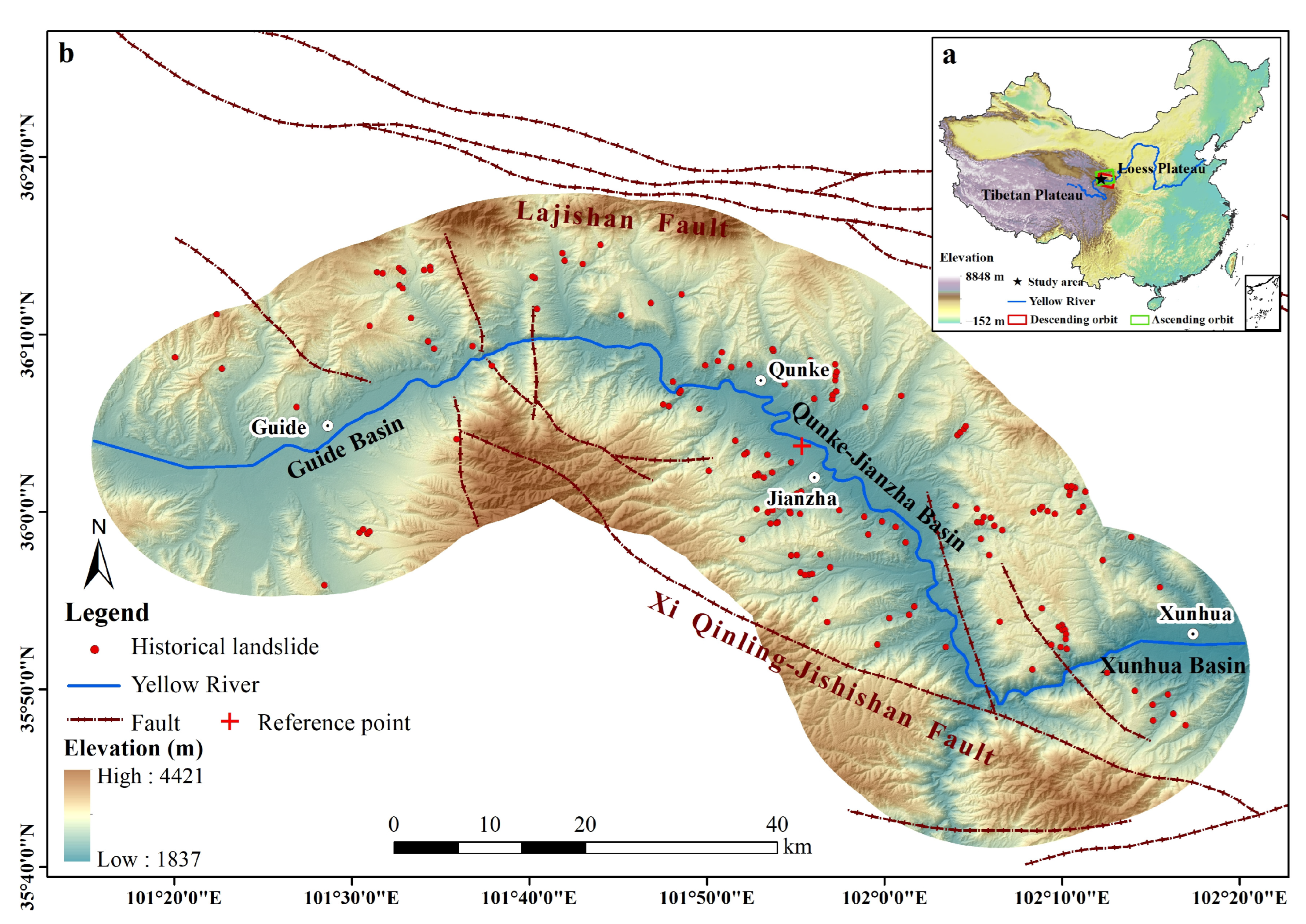
2. Study Area
3. Data and Methods
3.1. Ground Deformation Detection Using MTI
3.2. Hot Spot Analysis
3.3. Modeling Algorithms
3.3.1. CNN Model
3.3.2. RF Model
3.4. Modeling Factors
3.4.1. Discretizing of Continuous Data
3.4.2. Topographic and Geomorphic Factors
3.4.3. Hydrological Factors
3.4.4. Geological Factors
3.4.5. Human Activity Factors
3.4.6. IPTA Time Series Deformation Trend
4. Results
4.1. Ground Deformation Detection Using InSAR Technology
4.2. Extraction of Potential Landslide Candidates via Hot Spot Analysis
4.3. Modeling Process
4.3.1. Preparation of Potential Landslide Inventory
4.3.2. Selection of Conditioning Factors
4.3.3. Model Performance Evaluation Index
4.4. The Potential Landslides Classification Model
5. Discussion
5.1. Advantages of the Approach
5.2. Limitations and Further Directions of the Approach
6. Conclusions
Author Contributions
Funding
Data Availability Statement
Conflicts of Interest
References
- Confuorto, P.; Di Martire, D.; Infante, D.; Novellino, A.; Papa, R.; Calcaterra, D.; Ramondini, M. Monitoring of remedial works performance on landslide-affected areas through ground- and satellite-based techniques. CATENA 2019, 178, 77–89. [Google Scholar] [CrossRef]
- Bekaert, D.; Handwerger, A.; Agram, P.; Kirschbaum, D. InSAR-based detection method for mapping and monitoring slow-moving landslides in remote regions with steep and mountainous terrain: An application to Nepal. Remote Sens. Environ. 2020, 249, 111983. [Google Scholar] [CrossRef]
- Chen, C.; Xie, M.-W.; Jiang, Y.-J.; Jia, B.-N.; Du, Y. A new method for quantitative identification of potential landslide. Soils Found 2021, 61, 1475–1479. [Google Scholar] [CrossRef]
- Shen, Y.; Da, K.; Wu, M.; Zhou, G.; Wang, M.; Wang, T.; Xu, Q. Rapid and automatic detection of new potential landslide based on phase-gradient DInSAR. IEEE Geosci. Remote Sens. Lett. 2022, 19, 1–5. [Google Scholar]
- Sowers, G.F.; Royster, D.L. Field investigation. Spec. Rep. 1978, 176, 81–111. [Google Scholar]
- Zhang, Y.; Meng, X.; Chen, G.; Qiao, L.; Zeng, R.; Chang, J. Detection of geohazards in the Bailong River Basin using synthetic aperture radar interferometry. Landslides 2016, 13, 1273–1284. [Google Scholar] [CrossRef]
- Zhang, L.; Dai, K.; Deng, J.; Ge, D.; Liang, R.; Li, W.; Xu, Q. Identifying Potential Landslides by Stacking-InSAR in South-western China and Its Performance Comparison with SBAS-InSAR. Remote. Sens. 2021, 13, 3662. [Google Scholar] [CrossRef]
- Zhang, J.; Gong, Y.; Huang, W.; Wang, X.; Ke, Z.; Liu, Y.; Huo, A.; Adnan, A.; Abuarab, M.E.-S. Identification of Potential Landslide Hazards Using Time-Series InSAR in Xiji County, Ningxia. Water 2023, 15, 300. [Google Scholar] [CrossRef]
- Ciampalini, A.; Raspini, F.; Lagomarsino, D.; Catani, F.; Casagli, N. Landslide susceptibility map refinement using PSInSAR data. Remote. Sens. Envrion. 2016, 184, 302–315. [Google Scholar] [CrossRef]
- Li, C.; Fu, Z.; Wang, Y.; Tang, H.; Yan, J.; Gong, W.; Yao, W.; Criss, R.E. Susceptibility of reservoir-induced landslides and strategies for increasing the slope stability in the Three Gorges Reservoir Area: Zigui Basin as an example. Eng. Geol. 2019, 261, 105279. [Google Scholar] [CrossRef]
- Reichenbach, P.; Rossi, M.; Malamud, B.D.; Mihir, M.; Guzzetti, F. A review of statistically-based landslide susceptibility models. Earth Sci. Rev. 2018, 180, 60–91. [Google Scholar] [CrossRef]
- Zhao, F.; Meng, X.; Zhang, Y.; Chen, G.; Su, X.; Yue, D. Landslide Susceptibility Mapping of Karakorum Highway Combined with the Application of SBAS-InSAR Technology. Sensors 2019, 19, 2685. [Google Scholar] [CrossRef] [PubMed]
- He, Y.; Wang, W.; Zhang, L.; Chen, Y.; Chen, Y.; Chen, B.; He, X.; Zhao, Z. An identification method of potential landslide zones using InSAR data and landslide susceptibility. Geomat. Nat. Hazards Risk 2023, 14. [Google Scholar] [CrossRef]
- Merghadi, A.; Yunus, A.P.; Dou, J.; Whiteley, J.; ThaiPham, B.; Bui, D.T.; Avtar, R.; Abderrahmane, B. Machine learning methods for landslide susceptibility studies: A comparative overview of algorithm performance. Earth Sci. Rev. 2020, 207, 103225. [Google Scholar] [CrossRef]
- Naidu, S.; Sajinkumar, K.; Oommen, T.; Anuja, V.; Samuel, R.A.; Muraleedharan, C. Early warning system for shallow landslides using rainfall threshold and slope stability analysis. Geosci. Front. 2018, 9, 1871–1882. [Google Scholar] [CrossRef]
- Shiau, J.; Keawsawasvong, S. Multivariate adaptive regression splines analysis for 3D slope stability in anisotropic and het-erogenous clay. J. Rock Mech. Geotech. Eng. 2023, 15, 1052–1064. [Google Scholar] [CrossRef]
- Wasowski, J.; Bovenga, F. Remote sensing of landslide motion with emphasis on satellite multi-temporal interferometry applications: An overview. Landslide Hazards Risks Disasters 2022, 365–438. [Google Scholar]
- Zhang, Y.; Meng, X.; Dijkstra, T.; Jordan, C.; Chen, G.; Zeng, R.; Novellino, A. Forecasting the magnitude of potential landslides based on InSAR techniques. Remote. Sens. Environ. 2020, 241, 111738. [Google Scholar] [CrossRef]
- Wasowski, J.; Bovenga, F. Investigating landslides and unstable slopes with satellite Multi Temporal Interferometry: Current issues and future perspectives. Eng. Geol. 2014, 174, 103–138. [Google Scholar] [CrossRef]
- Tomás, R.; Pagán, J.I.; Navarro, J.A.; Cano, M.; Pastor, J.L.; Riquelme, A.; Cuevas-González, M.; Crosetto, M.; Barra, A.; Monserrat, O.; et al. Semi-Automatic Identification and Pre-Screening of Geological–Geotechnical Deformational Processes Using Persistent Scatterer Interferometry Datasets. Remote. Sens. 2019, 11, 1675. [Google Scholar] [CrossRef]
- Peng, J.; Ma, R.; Lu, Q.; Li, X.; Shao, T. Geological hazards effects of uplift of Qinghai-Tibet Plateau. Adv. Earth Sci. 2004, 19, 457–466. (In Chinese) [Google Scholar]
- Yin, Z.; Qin, X.; Zhao, W.; Wei., G. Characteristics of landslides of landslides in upper reaches of Yellow River with multiple data of remote sensing. J. Eng. Geol. 2013, 21, 779–787. (In Chinese) [Google Scholar]
- Yin, Z.; Qin, X.; Zhao, X.; Li, X.; Cheng, G.; Wei, G.; Shi, L.; Yuan, C. Temporal and Spatial Evolution and Triggering Mechanism of Landslide and Debris Flow in the Upper Reaches of the Yellow River; Science Press: Beijing, China, 2016. (In Chinese) [Google Scholar]
- Guo, X.; Wei, J.; Song, Z. Luminescence dating of a dammed lake formed by Ashegong landslide on the northeastern Tibetan Plateau. Quat. Int. 2022, 629, 74–80. [Google Scholar] [CrossRef]
- Shi, X.; Yang, C.; Zhang, L.; Jiang, H.; Liao, M.; Zhang, L.; Liu, X. Mapping and characterizing displacements of active loess slopes along the upstream Yellow River with multi-temporal InSAR datasets. Sci. Total Environ. 2019, 674, 200–210. [Google Scholar] [CrossRef] [PubMed]
- Qin, X.; Yin, Z.; Zhao, W. Xijitan Landslide in Guide Basin in the Upper Reaches of the Yellow River and its Dammed Lakes. Geophys. Remote Sens. 2015, 4, 2169-0049. [Google Scholar]
- Wei, G.; Yin, Z.; Ma, J.; Zhang, T. An analysis of forming stages and evolution process of the Ashigong landslide cluster in the upper reaches of the Yellow River. Hydrogeol. Eng. Geol. 2016, 43, 133–140. (In Chinese) [Google Scholar]
- Werner, C.; Wegmüller, U.; Strozzi, T.; Wiesmann, A. Interferometric point target analysis for deformation mapping. In Proceedings of the IGARSS 2003, Toulouse, France, 21–25 July 2003. [Google Scholar]
- Zhao, C.; Kang, Y.; Zhang, Q.; Lu, Z.; Li, B. Landslide Identification and Monitoring along the Jinsha River Catchment (Wudongde Reservoir Area), China, Using the InSAR Method. Remote. Sens. 2018, 10, 993. [Google Scholar] [CrossRef]
- Mantovani, M.; Devoto, S.; Piacentini, D.; Prampolini, M.; Soldati, M.; Pasuto, A. Advanced SAR Interferometric Analysis to Support Geomorphological Interpretation of Slow-Moving Coastal Landslides (Malta, Mediterranean Sea). Remote. Sens. 2016, 8, 443. [Google Scholar] [CrossRef]
- Getis, A.; Ord, J.K. The Analysis of Spatial Association by Use of Distance Statistics. Geogr. Anal. 2010, 24, 189–206. [Google Scholar] [CrossRef]
- Ord, J.K.; Getis, A. Local Spatial Autocorrelation Statistics: Distributional Issues and an Application. Geogr. Anal. 1995, 27, 286–306. [Google Scholar] [CrossRef]
- Lu, P.; Casagli, N.; Catani, F.; Tofani, V. Persistent Scatterers Interferometry Hotspot and Cluster Analysis (PSI-HCA) for detection of extremely slow-moving landslides. Int. J. Remote. Sens. 2011, 33, 466–489. [Google Scholar] [CrossRef]
- Silverman, B. Density Estimation for Statistics and Data Analysis; Chapman & Hall: London, UK, 1986. [Google Scholar]
- Yi, Y.; Zhang, Z.; Zhang, W.; Jia, H.; Zhang, J. Landslide susceptibility mapping using multiscale sampling strategy and convolutional neural network: A case study in Jiuzhaigou region. CATENA 2020, 195, 104851. [Google Scholar] [CrossRef]
- LeCun, Y.; Jackel, L.; Bottou, L.; Brunot, A.; Cortes, C.; Denker, J.; Drucker, H.; Guyon, I.; Miller, U.; Sackinger, E.; et al. Comparison of Learning Algorithms for Handwritten Digit Recognition. In Proceedings of the International Conference on Artificial Neural Network, Perth, Australia, 27 November–1 December 1995; Volume 60, pp. 53–60. [Google Scholar]
- Sameen, M.I.; Pradhan, B.; Lee, S. Application of convolutional neural networks featuring Bayesian optimization for landslide susceptibility assessment. CATENA 2020, 186, 104249. [Google Scholar] [CrossRef]
- Ngo, P.; Panahi, M.; Khosravi, K.; Ghorbanzadeh, O.; Kariminejad, N.; Cerda, A.; Lee, S. Evaluation of deep learning algo-rithms for national scale landslide susceptibility mapping of Iran. Geosci. Front. 2021, 12, 505–519. [Google Scholar]
- Fang, Z.; Wang, Y.; Peng, L.; Hong, H. Integration of convolutional neural network and conventional machine learning classifiers for landslide susceptibility mapping. Comput. Geosci 2020, 139, 104470. [Google Scholar] [CrossRef]
- Youssef, A.M.; Pradhan, B.; Dikshit, A.; Al-Katheri, M.M.; Matar, S.S.; Mahdi, A.M. Landslide susceptibility mapping using CNN-1D and 2D deep learning algorithms: Comparison of their performance at Asir Region, KSA. Bull. Eng. Geol. Environ. 2022, 81, 165. [Google Scholar] [CrossRef]
- Nair, V.; Hinton, G.E. Rectified linear units improve restricted Boltzmann machines. In Proceedings of the ICML-10: 27th International Conference on Machine Learning, Haifa, Israel, 21–24 June 2010; pp. 807–814. [Google Scholar]
- Hinton, G.E.; Srivastava, N.; Krizhevsky, A.; Sutskever, I.; Salakhutdinov, R.R. Improving neural networks by preventing co-adaptation of feature detectors. arXiv 2012, arXiv:1207.0580. [Google Scholar]
- Zhou, X.; Wen, H.; Zhang, Y.; Xu, J.; Zhang, W. Landslide susceptibility mapping using hybrid random forest with Ge-oDetector and RFE for factor optimization. Geosci. Front. 2021, 12, 101211. [Google Scholar] [CrossRef]
- Sun, D.; Wen, H.; Wang, D.; Xu, J. A random forest model of landslide susceptibility mapping based on hyperparameter optimization using Bayes algorithm. Geomorphology 2020, 362, 107201. [Google Scholar] [CrossRef]
- Stumpf, A.; Kerle, N. Object-oriented mapping of landslides using Random Forests. Remote. Sens. Environ. 2011, 115, 2564–2577. [Google Scholar] [CrossRef]
- Breiman, L. Random forests. Mach. Learn. 2001, 45, 5–32. [Google Scholar] [CrossRef]
- Wang, Y.; Fang, Z.; Hong, H. Comparison of convolutional neural networks for landslide susceptibility mapping in Yanshan County, China. Sci. Total Environ. 2019, 666, 975–993. [Google Scholar] [CrossRef]
- Deng, H.; Wu, L.Z.; Huang, R.Q.; Guo, X.G.; He, Q. Formation of the Siwanli ancient landslide in the Dadu River, China. Landslides 2016, 14, 385–394. [Google Scholar] [CrossRef]
- Liu, J.; Duan, Z. Quantitative Assessment of Landslide Susceptibility Comparing Statistical Index, Index of Entropy, and Weights of Evidence in the Shangnan Area, China. Entropy 2018, 20, 868. [Google Scholar] [CrossRef]
- Xiao, T.; Yin, K.; Yao, T.; Liu, S. Spatial prediction of landslide susceptibility using GIS-based statistical and machine learning models in Wanzhou County, Three Gorges Reservoir, China. Acta Geochim. 2019, 38, 654–669. [Google Scholar] [CrossRef]
- Rosati, S.; Balestra, G.; Giannini, V.; Mazzetti, S.; Russo, F.; Regge, D. ChiMerge discretization method: Impact on a computer aided diagnosis system for prostate cancer in MRI. In Proceedings of the IEEE International Symposium on Medical Measurements and Applications (MeMeA) Proceedings, Turin, Italy, 7–9 May 2015; pp. 297–302. [Google Scholar]
- Kerber, R. Chimerge: Discretization of numeric attributes. In Proceedings of the Tenth National Conference on Artificial Intelli-gence, San Jose, CA, USA, 12–16 July 1992; pp. 123–128. [Google Scholar]
- Peker, N.; Kubat, C. Application of Chi-square discretization algorithms to ensemble classification methods. Expert Syst. Appl. 2021, 185, 115540. [Google Scholar] [CrossRef]
- Li, F.; Yang, M.; Li, Y.; Zhang, M.; Wang, W.; Yuan, D.; Tang, D. An improved clear cell renal cell carcinoma stage prediction model based on gene sets. BMC Bioinform. 2020, 21, 232. [Google Scholar] [CrossRef]
- Conforti, M.; Pascale, S.; Robustelli, G.; Sdao, F. Evaluation of prediction capability of the artificial neural networks for mapping landslide susceptibility in the Turbolo River catchment (northern Calabria, Italy). CATENA 2014, 113, 236–250. [Google Scholar] [CrossRef]
- Moosavi, V.; Niazi, Y. Development of hybrid wavelet packet-statistical models (WP-SM) for landslide susceptibility map-ping. Landslides 2016, 13, 97–114. [Google Scholar] [CrossRef]
- Guo, Z.; Yin, K.; Fu, S.; Huang, F.; Gui, L.; Xia, H. Evaluation of Landslide Susceptibility Based on GIS and WOE⁃ BP Model. Earth Sci. 2019, 44, 4299–4312. [Google Scholar]
- Kutlug Sahin, E.; Colkesen, I. Performance analysis of advanced decision tree-based ensemble learning algorithms for land-slide susceptibility mapping. Geocarto Int. 2021, 36, 1253–1275. [Google Scholar] [CrossRef]
- Dou, J.; Yunus, A.P.; Bui, D.T.; Merghadi, A.; Sahana, M.; Zhu, Z.; Chen, C.-W.; Khosravi, K.; Yang, Y.; Pham, B.T. Assessment of advanced random forest and decision tree algorithms for modeling rainfall-induced landslide susceptibility in the Izu-Oshima Volcanic Island, Japan. Sci. Total Environ. 2019, 662, 332–346. [Google Scholar] [CrossRef] [PubMed]
- Aghdam, I.N.; Varzandeh, M.H.M.; Pradhan, B. Landslide susceptibility mapping using an ensemble statistical index (Wi) and adaptive neuro-fuzzy inference system (ANFIS) model at Alborz Mountains (Iran). Environ. Earth Sci. 2016, 75, 553. [Google Scholar] [CrossRef]
- Juliev, M.; Mergili, M.; Mondal, I.; Nurtaev, B.; Pulatov, A.; Hübl, J. Comparative analysis of statistical methods for landslide susceptibility mapping in the Bostanlik District, Uzbekistan. Sci. Total Environ. 2018, 653, 801–814. [Google Scholar] [CrossRef] [PubMed]
- Oh, H.-J.; Kadavi, P.R.; Lee, C.-W.; Lee, S. Evaluation of landslide susceptibility mapping by evidential belief function, logistic regression and support vector machine models. Geomat. Nat. Hazards Risk 2018, 9, 1053–1070. [Google Scholar] [CrossRef]
- Mokarram, M.; Roshan, G.; Negahban, S. Landform classification using topography position index (case study: Salt dome of Korsia-Darab plain, Iran). Model. Earth Syst. Environ. 2015, 1, 1–7. [Google Scholar] [CrossRef]
- Kadavi, P.R.; Lee, C.-W.; Lee, S. Application of Ensemble-Based Machine Learning Models to Landslide Susceptibility Mapping. Remote. Sens. 2018, 10, 1252. [Google Scholar] [CrossRef]
- Saleem, N.; Huq, M.E.; Twumasi, N.Y.D.; Javed, A.; Sajjad, A. Parameters Derived from and/or Used with Digital Elevation Models (DEMs) for Landslide Susceptibility Mapping and Landslide Risk Assessment: A Review. ISPRS Int. J. Geo Inf. 2019, 8, 545. [Google Scholar] [CrossRef]
- Shirvani, Z. A Holistic Analysis for Landslide Susceptibility Mapping Applying Geographic Object-Based Random Forest: A Comparison between Protected and Non-Protected Forests. Remote. Sens. 2020, 12, 434. [Google Scholar] [CrossRef]
- Park, S.; Kim, J. Landslide Susceptibility Mapping Based on Random Forest and Boosted Regression Tree Models, and a Comparison of Their Performance. Appl. Sci. 2019, 9, 942. [Google Scholar] [CrossRef]
- Kincal, C.; Kayhan, H. A Combined Method for Preparation of Landslide Susceptibility Map in Izmir (Türkiye). Appl. Sci. 2022, 12, 9029. [Google Scholar] [CrossRef]
- Jebur, M.N.; Pradhan, B.; Tehrany, M.S. Optimization of landslide conditioning factors using very high-resolution airborne laser scanning (LiDAR) data at catchment scale. Remote. Sens. Environ. 2014, 152, 150–165. [Google Scholar] [CrossRef]
- Zhang, K.; Wu, X.; Niu, R.; Yang, K.; Zhao, L. The assessment of landslide susceptibility mapping using random forest and decision tree methods in the Three Gorges Reservoir area, China. Environ. Earth Sci. 2017, 76, 405. [Google Scholar] [CrossRef]
- Chapi, K.; Singh, V.P.; Shirzadi, A.; Shahabi, H.; Bui, D.T.; Pham, B.T.; Khosravi, K. A novel hybrid artificial intelligence approach for flood susceptibility assessment. Environ. Model. Softw. 2017, 95, 229–245. [Google Scholar] [CrossRef]
- Ballerine, C. Topographic Wetness Index Urban Flooding Awareness Act Action Support: Will & DuPage Counties, Illinois; Illinois State Water Survey: Champaign, IL, USA, 2017. [Google Scholar]
- Borga, M.; Dalla Fontana, G.; Cazorzi, F. Analysis of topographic and climatic control on rainfall-triggered shallow land-sliding using a quasi-dynamic wetness index. J. Hydrol. 2002, 268, 56–71. [Google Scholar] [CrossRef]
- Zhao, Y.; Wang, R.; Jiang, Y. GIS-based logistic regression for rainfall-induced landslide susceptibility mapping under dif-ferent grid sizes in Yueqing, Southeastern China. Eng. Geol. 2019, 259, 105147. [Google Scholar] [CrossRef]
- Huang, F.; Yin, K.; Huang, J.; Gui, L.; Wang, P. Landslide susceptibility mapping based on self-organizing-map network and extreme learning machine. Eng. Geol. 2017, 223, 11–22. [Google Scholar] [CrossRef]
- Youssef, A.M.; Pourghasemi, H.R. Landslide susceptibility mapping using machine learning algorithms and comparison of their performance at Abha Basin, Asir Region, Saudi Arabia. Geosci. Front. 2020, 12, 639–655. [Google Scholar] [CrossRef]
- Zhou, B.; Hu, G.; Peng, J.; Lv, B. Landslide risk assessment of Lagan Gorge-Sigou Gorge section in the upper reaches of the Yellow River Based on GIS. South North Water Transf. Water Sci. Technol. 2010, 8, 36–38+48. (In Chinese) [Google Scholar]
- Bucci, F.; Santangelo, M.; Cardinali, M.; Fiorucci, F.; Guzzetti, F. Landslide distribution and size in response to Quaternary fault activity: The Peloritani Range, NE Sicily, Italy. Earth Surf. Process. Landf. 2016, 41, 711–720. [Google Scholar] [CrossRef]
- Guo, X.; Wei, J.; Lu, Y.; Song, Z.; Liu, H. Geomorphic Effects of a Dammed Pleistocene Lake Formed by Landslides along the Upper Yellow River. Water 2020, 12, 1350. [Google Scholar] [CrossRef]
- Nedbal, V.; Brom, J. Impact of highway construction on land surface energy balance and local climate derived from LANDSAT satellite data. Sci. Total Environ. 2018, 633, 658–667. [Google Scholar] [CrossRef] [PubMed]
- Karra, K.; Kontgis, C.; Statman-Weil, Z.; Mazzariello, J.C.; Mathis, M.; Brumby, S. Global land use/land cover with Sentinel 2 and deep learning. IEEE Geosci. Remote Sens. Soc. 2021, 4704–4707. [Google Scholar] [CrossRef]
- Cigna, F.; Del Ventisette, C.; Liguori, V.; Casagli, N. Advanced radar-interpretation of InSAR time series for mapping and characterization of geological processes. Nat. Hazards Earth Syst. Sci. 2011, 11, 865–881. [Google Scholar] [CrossRef]
- Iannacone, J.P.; Corsini, A.; Berti, M.; Morgan, J.; Falorni, G. Characterization of Longwall Mining Induced Subsidence by Means of Automated Analysis of InSAR Time-Series. In Engineering Geology for Society and Territory; Springer: Berlin/Heidelberg, Germany, 2015; Volume 5, pp. 973–977. [Google Scholar]
- Berti, M.; Corsini, A.; Franceschini, S.; Iannacone, J.P. Automated classification of Persistent Scatterers Interferometry time series. Nat. Hazards Earth Syst. Sci. 2013, 13, 1945–1958. [Google Scholar] [CrossRef]
- Lu, P.; Bai, S.; Tofani, V.; Casagli, N. Landslides detection through optimized hot spot analysis on persistent scatterers and distributed scatterers. ISPRS J. Photogramm. Remote. Sens. 2019, 156, 147–159. [Google Scholar] [CrossRef]
- Zhang, Y.; Meng, X.; Jordan, C.; Novellino, A.; Dijkstra, T.; Chen, G. Investigating slow-moving landslides in the Zhouqu region of China using InSAR time series. Landslides 2018, 15, 1299–1315. [Google Scholar] [CrossRef]
- Liang, J.; Dong, J.; Zhang, S.; Zhao, C.; Liu, B.; Yang, L.; Yan, S.; Ma, X. Discussion on InSAR Identification Effectivity of Potential Landslides and Factors That Influence the Effectivity. Remote. Sens. 2022, 14, 1952. [Google Scholar] [CrossRef]
- Dou, J.; Yunus, A.P.; Bui, D.T.; Merghadi, A.; Sahana, M.; Zhu, Z.; Chen, C.-W.; Han, Z.; Pham, B.T. Improved landslide assessment using support vector machine with bagging, boosting, and stacking ensemble machine learning framework in a mountainous watershed, Japan. Landslides 2020, 17, 641–658. [Google Scholar] [CrossRef]
- He, Q.; Wang, M.; Liu, K. Rapidly assessing earthquake-induced landslide susceptibility on a global scale using random forest. Geomorphology 2021, 391, 107889. [Google Scholar] [CrossRef]
- Yu, L.; Cao, Y.; Zhou, C.; Wang, Y.; Huo, Z. Landslide Susceptibility Mapping Combining Information Gain Ratio and Support Vector Machines: A Case Study from Wushan Segment in the Three Gorges Reservoir Area, China. Appl. Sci. 2019, 9, 4756. [Google Scholar] [CrossRef]
- Hong, H.; Liu, J.; Zhu, A. Modeling landslide susceptibility using LogitBoost alternating decision trees and forest by penalizing attributes with the bagging ensemble. Sci. Total Environ. 2020, 718, 137231. [Google Scholar] [CrossRef] [PubMed]
- Kalantar, B.; Ueda, N.; Saeidi, V.; Ahmadi, K.; Halin, A.; Shabani, F. Landslide susceptibility mapping: Machine and en-semble learning based on remote sensing big data. Remote Sens. 2020, 12, 1737. [Google Scholar] [CrossRef]
- Bui, D.T.; Tuan, T.A.; Klempe, H.; Pradhan, B.; Revhaug, I. Spatial prediction models for shallow landslide hazards: A comparative assessment of the efficacy of support vector machines, artificial neural networks, kernel logistic regression, and logistic model tree. Landslides 2015, 13, 361–378. [Google Scholar] [CrossRef]
- Frattini, P.; Crosta, G.; Carrara, A. Techniques for evaluating the performance of landslide susceptibility models. Eng. Geol. 2010, 111, 62–72. [Google Scholar] [CrossRef]
- Arabameri, A.; Saha, S.; Roy, J.; Chen, W.; Blaschke, T.; Bui, D.T. Landslide Susceptibility Evaluation and Management Using Different Machine Learning Methods in The Gallicash River Watershed, Iran. Remote. Sens. 2020, 12, 475. [Google Scholar] [CrossRef]
- Liang, Z.; Wang, C.; Khan, K.U.J. Application and comparison of different ensemble learning machines combining with a novel sampling strategy for shallow landslide susceptibility mapping. Stoch. Environ. Res. Risk Assess 2020, 35, 1243–1256. [Google Scholar] [CrossRef]
- Saha, S.; Roy, J.; Pradhan, B.; Hembram, T.K. Hybrid ensemble machine learning approaches for landslide susceptibility mapping using different sampling ratios at East Sikkim Himalayan, India. Adv. Space Res. 2021, 68, 2819–2840. [Google Scholar] [CrossRef]
- Gao, H.; Fam, P.S.; Tay, L.T.; Low, H.C. Comparative landslide spatial research based on various sample sizes and ratios in Penang Island, Malaysia. Bull. Eng. Geol. Environ. 2020, 80, 851–872. [Google Scholar] [CrossRef]
- Bragagnolo, L.; Rezende, L.; da Silva, R.; Grzybowski, J. Convolutional neural networks applied to semantic segmentation of landslide scars. CATENA 2021, 201, 1. [Google Scholar] [CrossRef]
- Zeng, X.; Wen, S.; Zeng, Z.; Huang, T. Design of memristor-based image convolution calculation in convolutional neural network. Neural Comput. Appl. 2016, 30, 503–508. [Google Scholar] [CrossRef]
- Sui, D.Z. Tobler’s first law of geography: A big idea for a small world? Ann. Assoc. Am. Geogr. 2004, 94, 269–277. [Google Scholar] [CrossRef]
- Jiang, Z.; Wang, M.; Liu, K. Comparisons of Convolutional Neural Network and Other Machine Learning Methods in Landslide Susceptibility Assessment: A Case Study in Pingwu. Remote. Sens. 2023, 15, 798. [Google Scholar] [CrossRef]
- Rouyet, L.; Lauknes, T.R.; Christiansen, H.H.; Strand, S.M.; Larsen, Y. Seasonal dynamics of a permafrost landscape, Adventdalen, Svalbard, investigated by InSAR. Remote. Sens. Environ. 2019, 231, 111236. [Google Scholar] [CrossRef]
- Van Den Eeckhaut, M.; Poesen, J.; Verstraeten, G.; Vanacker, V.; Moeyersons, J.; Nyssen, J.; Van Beek, L.P.H. The Effec-tiveness of Hillshade Maps and Expert Knowledge in Mapping Old Deep-Seated Landslides. Geomorphology 2005, 67, 351–363. [Google Scholar] [CrossRef]
- Xun, Z.; Zhao, C.; Kang, Y.; Liu, X.; Liu, Y.; Du, C. Automatic Extraction of Potential Landslides by Integrating an Optical Remote Sensing Image with an InSAR-Derived Deformation Map. Remote Sens. 2022, 14, 2669. [Google Scholar] [CrossRef]
- Ye, Z.; Yang, K.; Lin, Y.; Guo, S.; Sun, Y.; Chen, X.; Lai, R.; Zhang, H. A comparison between Pixel-based deep learning and Object-based image analysis (OBIA) for individual detection of cabbage plants based on UAV Visible-light images. Comput. Electron. Agric. 2023, 209, 107822. [Google Scholar] [CrossRef]
- Tang, Y.; Feng, F.; Guo, Z.; Feng, W.; Li, Z.; Wang, J.; Sun, Q.; Ma, H.; Li, Y. Integrating principal component analysis with statistically-based models for analysis of causal factors and landslide susceptibility mapping: A comparative study from the loess plateau area in Shanxi (China). J. Clean. Prod. 2020, 277, 124159. [Google Scholar] [CrossRef]
- Zhu, J.; Hu, J.; Li, Z.; Sun, Q.; Zheng, W. Recent progress in landslide monitoring with InSAR. Acta Geod. Et Car-Tographica Sin. 2022, 5, 2001. [Google Scholar]
- Cigna, F.; Bateson, L.; Jordan, C.; Dashwood, C. Simulating SAR geometric distortions and predicting Persistent Scatterer densities for ERS-1/2 and ENVISAT C-band SAR and InSAR applications: Nationwide feasibility assessment to monitor the landmass of Great Britain with SAR imagery. Remote Sens. Environ. 2014, 152, 441–466. [Google Scholar] [CrossRef]
- Li, Y.; Zuo, X.; Zhu, D.; Wu, W.; Yang, X.; Guo, S.; Shi, C.; Huang, C.; Li, F.; Liu, X. Identification and Analysis of Landslides in the Ahai Reservoir Area of the Jinsha River Basin Using a Combination of DS-InSAR, Optical Images, and Field Surveys. Remote Sens. 2022, 14, 6274. [Google Scholar] [CrossRef]
- Wang, Y.; Cui, X.; Che, Y.; Li, P.; Jiang, Y.; Peng, X. Automatic Identification of Slope Active Deformation Areas in the Zhouqu Region of China With DS-InSAR Results. Front. Environ. Sci. 2022, 10, 883427. [Google Scholar] [CrossRef]
- Li, Z.; Dai, K.; Deng, J.; Liu, C.; Shi, X.; Tang, G.; Yin, T. Identifying Potential Landslides in Steep Mountainous Areas Based on Improved Seasonal Interferometry Stacking-InSAR. Remote Sens. 2023, 15, 3278. [Google Scholar] [CrossRef]
- Cao, N.; Lee, H.; Jung, H.C. A Phase-Decomposition-Based PSInSAR Processing Method. IEEE Trans. Geosci. Remote. Sens. 2016, 54, 1074–1090. [Google Scholar] [CrossRef]
- Dong, J.; Zhang, L.; Tang, M.; Liao, M.; Xu, Q.; Gong, J.; Ao, M. Mapping landslide surface displacements with time series SAR interferometry by combining persistent and distributed scatterers: A case study of Jiaju landslide in Danba, China. Remote Sens. Environ. 2018, 205, 180–198. [Google Scholar] [CrossRef]
- Jia, H.; Wang, Y.; Ge, D.; Deng, Y.; Wang, R. Improved offset tracking for predisaster deformation monitoring of the 2018 Jinsha River landslide (Tibet, China). Remote. Sens. Environ. 2020, 247, 111899. [Google Scholar] [CrossRef]
- Wang, Q.; Yu, W.; Xu, B.; Wei, G. Assessing the Use of GACOS Products for SBAS-InSAR Deformation Monitoring: A Case in Southern California. Sensors-Basel 2019, 19, 3894. [Google Scholar] [CrossRef]
- Abe, T.; Iwahana, G.; Efremov, P.V.; Desyatkin, A.R.; Kawamura, T.; Fedorov, A.; Zhegusov, Y.; Yanagiya, K.; Tadono, T. Surface displacement revealed by L-band InSAR analysis in the Mayya area, Central Yakutia, underlain by continuous permafrost. Earth Planets Space 2020, 72, 1–16. [Google Scholar] [CrossRef]
- Su, X.; Zhang, Y.; Meng, X.; Rehman, M.U.; Khalid, Z.; Yue, D. Updating Inventory, Deformation, and Development Characteristics of Landslides in Hunza Valley, NW Karakoram, Pakistan by SBAS-InSAR. Remote. Sens. 2022, 14, 4907. [Google Scholar] [CrossRef]
- Li, H.; He, Y.; Xu, Q.; Deng, J.; Li, W.; Wei, Y.; Zhou, J. Sematic segmentation of loess landslides with STAPLE mask and fully connected conditional random field. Landslides 2023, 20, 367–380. [Google Scholar] [CrossRef]


| Models | Accuracy | Precision | Recall | AUC |
|---|---|---|---|---|
| RF | 0.67 | 0.64 | 0.74 | 0.73 |
| CNN | 0.75 | 0.75 | 0.82 | 0.75 |
Disclaimer/Publisher’s Note: The statements, opinions and data contained in all publications are solely those of the individual author(s) and contributor(s) and not of MDPI and/or the editor(s). MDPI and/or the editor(s) disclaim responsibility for any injury to people or property resulting from any ideas, methods, instructions or products referred to in the content. |
© 2023 by the authors. Licensee MDPI, Basel, Switzerland. This article is an open access article distributed under the terms and conditions of the Creative Commons Attribution (CC BY) license (https://creativecommons.org/licenses/by/4.0/).
Share and Cite
Zhang, Y.; Li, Y.; Meng, X.; Liu, W.; Wang, A.; Liang, Y.; Su, X.; Zeng, R.; Chen, X. Automatic Mapping of Potential Landslides Using Satellite Multitemporal Interferometry. Remote Sens. 2023, 15, 4951. https://doi.org/10.3390/rs15204951
Zhang Y, Li Y, Meng X, Liu W, Wang A, Liang Y, Su X, Zeng R, Chen X. Automatic Mapping of Potential Landslides Using Satellite Multitemporal Interferometry. Remote Sensing. 2023; 15(20):4951. https://doi.org/10.3390/rs15204951
Chicago/Turabian StyleZhang, Yi, Yuanxi Li, Xingmin Meng, Wangcai Liu, Aijie Wang, Yiwen Liang, Xiaojun Su, Runqiang Zeng, and Xu Chen. 2023. "Automatic Mapping of Potential Landslides Using Satellite Multitemporal Interferometry" Remote Sensing 15, no. 20: 4951. https://doi.org/10.3390/rs15204951