Signal Occlusion-Resistant Satellite Selection for Global Navigation Applications Using Large-Scale LEO Constellations

Abstract

With the continuous construction of large-scale Low Earth Orbit (LEO) constellations, their potential for Global Navigation Satellite System (GNSS) applications has been emphasized. This study aims to derive an optimal positioning configuration formula based on the ratio of high-elevation and low-elevation satellites, which can improve the positioning accuracy and overcome the accuracy loss due to signal occlusion. A genetic algorithm is used to solve the optimal positioning configuration problem for large-scale satellite selection. Through a simulation using Starlink satellites currently in orbit, it is verified that the traditional recursive algorithm cannot be applied to satellite selection for large-scale constellations. The proposed formula has a similar accuracy to the Quasi-Optimal algorithm when there is no signal occlusion and the satellites are uniformly selected. However, the accuracy of the latter deteriorates significantly under signal occlusion. Our algorithm can effectively overcome this problem. Moreover, we discuss the effect of different types of obstructions on the accuracy loss. We find that the Quasi-Optimal algorithm is more sensitive to a single large-angle obstruction than multiple small-angle obstructions. Our proposed formula can reduce the localization accuracy degradation caused by signal occlusions in both scenarios.

1. Introduction

With many large-scale Low Earth Orbit (LEO) constellation projects launched, such as Iridium, SpaceX, OneWeb, and Hongyan, LEO satellites have recently received attention concerning their prospects of augmenting the Global Navigation Satellite System (GNSS). The large-scale LEO constellation greatly increases the number of visible satellites, which offers both opportunities and challenges for the GNSS system. More satellites enable more favorable geometric configurations for positioning, thus reducing the Geometric Dilution of Precision (GDOP) and improving the positioning results under occluded conditions. However, they also impose new burdens and challenges on the receivers. Therefore, how the optimal number of satellites can be selected from a large pool of candidates and how the receiver computation load can be balanced with the positioning accuracy is an urgent problem to be solved.

As GNSS satellite constellations continue to expand, the investigation into selecting appropriate satellites from among the visible ones has gained momentum. Several distinct technical approaches have emerged from this research. The initial approach involves determining the optimal satellite combination by assessing the influence of currently observable satellites on the overall GDOP. Subsequently, a recursive strategy is employed to finalize the optimal satellite constellation [1,2,3,4,5,6,7,8,9].

Contrastingly, the second technical approach acquires satellite selection outcomes directly by leveraging the geometric interactions among satellites. The principal strength of this method lies in its rapid and convenient nature. However, it does exhibit a certain deficiency in theoretical underpinning, relying more on empirical algorithms. Notably, within this category, the Quasi-Optimal algorithm, which eliminates satellites sharing a common line of sight [10,11], and the Fast algorithm [12], which achieves the optimal configuration of 4–8 satellites through exhaustive computer enumeration, stand out as the most prominent examples. These algorithms have subsequently formed the basis for a series of investigations into optimization selection methods [13,14,15].

The third approach involves delving into the theoretical examination of the GDOP. Prior research encompasses scrutinizing the closed-form formulation of the GDOP for multi-GNSS systems [16,17], investigating the correlation between the GDOP and user-to-satellite unit vectors [18] and refining the outcomes of approximate closed-form formulations using the PDOP (Position Dilution of Precision) [19]. Notably, optimal GDOP configurations have been explored as well. For instance, Xue et al. conducted an analysis of optimal GDOP configurations in underwater scenarios devoid of observation constraints [20]. Their findings underscored the pivotal roles that symmetry and uniformity play in achieving accurate positioning results. Moreover, Meng et al. and Xue et al. extended this line of inquiry by scrutinizing the optimal positioning configuration of a dual GNSS system under a 5-satellite scenario [21,22].

As technology continues to advance in the realm of artificial intelligence, there has been a progressive surge in studies exploring the application of intelligent algorithms to tackle GDOP challenges. For example, this surge includes the utilization of modified genetic algorithms [23], the implementation of end-to-end neural networks employing point cloud segmentation [24,25], the integration of adaptive simulated annealing particle swarm optimization algorithms [26], the application of improved particle swarm optimization algorithms [27], the utilization of the easy binary particle swarm optimization with a queen informant (EPSOq) algorithm to address GDOP optimization distribution [28], and the combination of unsupervised learning with the Fast algorithm to tackle satellite distribution challenges [29].

Simultaneously, research endeavors focused on incorporating additional parameters, such as Receiver Autonomous Integrity Monitoring (RAIM) [30,31,32] and a Weighted Geometric Dilution of Precision (WGDOP) system [33,34], among other considerations [35,36,37,38], are also on the rise.

The recursive method is difficult to apply in large-scale satellite constellations, and it requires too much computing power to move from high resolution to low resolution. The traditional algorithm assumes that the satellite positions are uniformly distributed, which lacks a theoretical basis. It is also incapable of handling the influence of obstructions in a complex working environment. The optimal distributions of satellites derived from theoretical analyses are symmetric with respect to the observing point. However, satellites at a negative angle cannot be observed under the GNSS observing scenarios. Therefore, there is a need to investigate the theory and obtain the preferred satellite distribution combinations under GNSS operation. A suitable optimization method is also examined to minimize the influence of obstructions according to the theory. The biggest problem with intelligent algorithms at present is that algorithms with fast computational speed require training and specify the number of satellites to be finally selected during training, while algorithms that do not require pre-training have poor budget speeds and are not well adapted to scenarios where large-scale LEO satellite constellations are used. Therefore, in the field of large-scale LEO satellite constellation positioning in the foreseeable future, it is necessary to derive configurations with the lowest GDOP through theoretical research and, at the same time, based on the results of the theoretical research, to propose an effective and efficient positioning satellite selection algorithm that can mitigate the influence of obstructions.

The remainder of this study is organized as follows. Section 2 briefly introduces the criterion of the GDOP, traditional recursive algorithms for mathematically intractable GDOP problems, and the concept of classical genetic algorithm. In Section 3, configurations with the lowest GDOP are mathematically derived. A satellite selection algorithm incorporating a genetic algorithm is presented based on the derived formulas to overcome the effect of obstruction. In Section 4, real-world Starlink satellite data are used to analyze the performance of the proposed algorithm. Lastly, in Section 5, the content of this study is summarized, and the conclusions are presented.

2. The Geometric Dilution of Precision and Genetic Algorithm

2.1. GDOP Criterion

The apparent distance $\rho$ between the receiver and the satellite at a given instant of time is known as the pseudorange. The pseudorange ${\rho }_c^{\left(k\right)}$ is eliminated by compensating for satellite clock error and residual errors as much as possible, as in the following equation.

$$\begin{array}{c}\hfill {\rho }_c^{\left(k\right)}=r^{\left(k\right)}+c·\delta t_u+{\tilde{\epsilon }}_{\rho }^{\left(k\right)}\end{array}$$

(1)

${\tilde{\epsilon }}_{\rho }^{\left(k\right)}$ represents a comprehensive impact of residual errors.

Let $\mathit{x}=(x,y,z)$ and ${\mathit{x}}^{\left(k\right)}=\left(x^{\left(k\right)},y^{\left(k\right)},z^{\left(k\right)}\right)$ be the vectors representing the location of the receiver and the $k^{th}$ satellite at the time of measurement and signal emission, respectively, where $k=1,2,\dots ,K$. The true range between the receiver and the satellite is then given by

$$\begin{array}{c}\hfill \begin{array}{cc}\hfill r^{\left(k\right)}& =\sqrt{{\left(x^{\left(k\right)}-x\right)}^2+{\left(y^{\left(k\right)}-y\right)}^2+{\left(z^{\left(k\right)}-z\right)}^2}\hfill \\ & =∥{\mathit{x}}^{\left(k\right)}-\mathit{x}∥\hfill \end{array}\end{array}$$

(2)

Thus,

$$\begin{array}{c}\hfill {\rho }_c^{\left(k\right)}=∥{\mathit{x}}^{\left(k\right)}-\mathit{x}∥+b+{\tilde{\epsilon }}_{\rho }^{\left(k\right)}\end{array}$$

(3)

where b is a parameter that accounts for the receiver clock bias $c·\delta t_{\mathrm{u}}$.

Given K pseudorange measurements from different satellites, each of which is a nonlinear equation, as in Equation (2), we have four unknowns to solve: three components of $\mathit{x}$ and b. Therefore, we need at least four equations to determine the unknowns. This implies that the receiver position can be computed only if pseudoranges from at least four satellites are simultaneously available, and in general, no additional information is needed to estimate the receiver clock bias.

A straightforward way to solve the K nonlinear Equation (2) is to linearize it around an initial guess of the user position and then apply an iterative method. We use the Newton–Raphson method for this purpose. Suppose ${\mathit{x}}_0=\left(x_0,y_0,z_0\right)$ and $b_0$ are the initial estimates of the user position and receiver clock bias, respectively. Therefore, from Equation (3), we can obtain the corrected pseudorange measurement for the $k^{th}$ satellite, denoted by ${\rho }_c^{\left(k\right)}$. This is compared with the approximate pseudorange value ${\rho }_0^{\left(k\right)}$ that corresponds to ${\mathit{x}}_0$ and $b_0$.

$$\begin{array}{c}\hfill {\rho }_0^{\left(k\right)}=∥{\mathit{x}}^{\left(k\right)}-{\mathit{x}}_0∥+b_0\end{array}$$

(4)

We can write $\mathit{x}={\mathit{x}}_0+\delta \mathit{x}$ and $b=b_0+\delta b$, denoting $\delta \mathit{x}$ and $\delta b$ as the corrections to the initial estimates. We can then set up a linear system of equations to solve for $\delta \mathit{x}$ and $\delta b$.

$$\begin{array}{cc}\hfill \delta {\rho }^{\left(k\right)}& ={\rho }_c^{\left(k\right)}-{\rho }_0^{\left(k\right)}\hfill \\ & =∥{\mathit{x}}^{\left(k\right)}-{\mathit{x}}_0-\delta \mathit{x}∥-∥{\mathit{x}}^{\left(k\right)}-{\mathit{x}}_0∥+\left(b-b_0\right)+{\tilde{\epsilon }}_{\rho }^{\left(k\right)}\hfill \\ & \approx -\frac{\left({\mathit{x}}^{\left(k\right)}-{\mathit{x}}_0\right)}{∥{\mathit{x}}^{\left(k\right)}-{\mathit{x}}_0∥}·\delta \mathit{x}+\delta b+{\tilde{\epsilon }}_{\rho }^{\left(k\right)}\hfill \\ & =-{\mathbf{1}}^{\left(k\right)}·\delta \mathit{x}+\delta b+{\tilde{\epsilon }}_{\rho }^{\left(k\right)}\hfill \end{array}$$

(5)

We use the Taylor series expansion to approximate the vector form of the equations. In Equation (5), ${\mathbf{1}}^{\left(k\right)}$ denotes the unit vector pointing from the receiver’s initial estimated position to the $k^{th}$ satellite, and each component of ${\mathbf{1}}^{\left(k\right)}$ is the direction cosine of the vector from the receiver’s estimated position to the satellite direction.

$$\begin{array}{c}\hfill {\mathbf{1}}^{\left(k\right)}=\frac{1}{∥{\mathit{x}}^{\left(k\right)}-{\mathit{x}}_0∥}{\left(x^{\left(k\right)}-x_0,y^{\left(k\right)}-y_0,z^{\left(k\right)}-z_0\right)}^{\mathrm{T}}\end{array}$$

(6)

The K linear Equation (6) can be expressed in matrix notation as

$$\begin{array}{c}\hfill \delta \rho =\left. [\begin{array}{c}\delta {\rho }^{\left(1\right)}\\ \delta {\rho }^{\left(2\right)}\\ ⋮\\ \delta {\rho }^{\left(K\right)}\end{array}\right]=\left. [\begin{array}{cc}{\left(-{\mathbf{1}}^{\left(1\right)}\right)}^{\mathrm{T}}& 1\\ {\left(-{\mathbf{1}}^{\left(2\right)}\right)}^{\mathrm{T}}& 1\\ ⋮& \\ {\left(-{\mathbf{1}}^{\left(K\right)}\right)}^{\mathrm{T}}& 1\end{array}\right]\left. [\begin{array}{c}\delta \mathit{x}\\ \delta b\end{array}\right]+{\tilde{\epsilon }}_{\rho }\end{array}$$

(7)

There are four unknowns in the K (at least 4) linear equations: $\delta \mathit{x}$ and $\delta b$. Moreover, Equation (7) can be reduced to

$$\begin{array}{c}\hfill \delta \rho =\mathit{G}\left. [\begin{array}{c}\delta \mathit{x}\hfill \\ \delta b\hfill \end{array}\right]+{\tilde{\epsilon }}_{\rho }\end{array}$$

(8)

$$\begin{array}{c}\hfill \begin{array}{cc}\hfill \mathit{F}& =\left. [\begin{array}{c}{\left(-{\mathbf{1}}^{\left(1\right)}\right)}^{\mathrm{T}}\\ {\left(-{\mathbf{1}}^{\left(2\right)}\right)}^{\mathrm{T}}\\ ⋮\\ {\left(-{\mathbf{1}}^{\left(K\right)}\right)}^{\mathrm{T}}\end{array}\right]\hfill \\ \hfill \mathit{G}& =\left. [\mathit{F}{\mathit{k}}_K\right]=\left. [\begin{array}{cc}{\left(-{\mathbf{1}}^{\left(1\right)}\right)}^{\mathrm{T}}& 1\\ {\left(-{\mathbf{1}}^{\left(2\right)}\right)}^{\mathrm{T}}& 1\\ ⋮& \\ {\left(-{\mathbf{1}}^{\left(K\right)}\right)}^{\mathrm{T}}& 1\end{array}\right],{\mathbf{k}}_K={\left. [\begin{array}{ccc}1\hfill & \dots \hfill & 1\hfill \end{array}\right]}^{\mathrm{T}}\hfill \end{array}\end{array}$$

(9)

$\mathit{G}$ is indicated as the $K\times 4$ geometry matrix that characterizes the geometric configuration of the user and the satellites. This is called the geometry matrix. If $K=4$, we can directly solve for the four unknowns using these four equations.

This happens when the equations are linearly dependent on each other, making $\mathit{G}$ a singular matrix. When the elevation angles of all the satellites observed at the user’s location are equal, and the rank of $\mathit{G}$ is three. The same problem arises when all of the line-of-sight vectors are coplanar. In this case, the satellites appear to be aligned in the sky view, which is unlikely in a GPS system of 24 or more satellites, and can change rapidly.

We can find the least squares solution to refine the initial estimate in Equation (8) when K is usually larger than 4 using the orthogonality principle. The new and improved user position and clock difference values are

$$\begin{array}{c}\hfill \begin{array}{c}\widehat{x}={\mathit{x}}_0+\delta \widehat{\mathit{x}}\hfill \\ \widehat{b}=b_0+\delta \widehat{b}\hfill \end{array}\end{array}$$

(10)

The system of observation equations can be linearized around the updated user position and clock bias estimates by repeating the solution of the equations until the change in the estimates is sufficiently small. Each iteration involves a new computation of the following parameters: (i) the GPS time t at which the signal is received, (ii) for each satellite, the signal travel time $t_r$, the transmission time $\left(t-t_r\right)$, and the corresponding satellite position as well as Equation (3), and (iii) the geometry matrix $\mathit{G}$. This estimation process converges fast and usually requires only two to four iterations.

In the above least squares computation, there is an implicit assumption that all measurements have equal accuracy. However, in reality, this assumption is hardly valid. The measurement errors from satellites with lower elevation satellites are usually larger than those from satellites with higher elevation angles. In fact, the measured pseudoranges are not only unequal in accuracy but also correlated with each other when applying a model to all observations referring to an epoch. If ionospheric and tropospheric delay models are applied, the delay errors in the zenith direction are proportional for all measurements, thus creating a correlation. Differential correction measurements are also correlated. In general, the stronger the correlation of the pseudorange error, the smaller the estimated position error is. In an extreme case, the common error of all measurements is absorbed in the computation of the clock bias and does not affect the position computation, but highly correlated parameters do not regularly lead to the correct determination of range/height. This can be seen in Equation (8).

Ideally, the mean vector and covariance matrix can characterize the errors in pseudorange measurements. With this structure, the minimum mean square error position estimate can be obtained, and the position error variance can be determined. However, it is usually very difficult to describe the measurement error in this way. For simplicity, the measurement errors from different satellites were assumed to be zero-mean, uncorrelated, and homoscedastic. Under such conditions, Equation (1) can be written as

$$\begin{array}{c}\hfill \begin{array}{c}\mathrm{E}\left({\tilde{\epsilon }}_{\rho }\right)=0\hfill \\ \mathrm{Cov}\left({\tilde{\epsilon }}_{\rho }\right)=\mathrm{E}\left({\tilde{\epsilon }}_{\rho }{\tilde{\epsilon }}_{\rho }^{\mathrm{T}}\right)={\sigma }_{\mathrm{URE}}^{2}I\hfill \end{array}\end{array}$$

(11)

where $\mathrm{E}\left(·\right)$ denotes the mean or expected value, $\mathrm{Cov}\left(·\right)$ denotes the covariance, I is the identity matrix, and ${\sigma }_{\mathrm{URE}}$ is the standard deviation of the user range error (URE) common to each satellite, which is simplified as $\sigma$. Strictly speaking, this assumption has not been verified in many cases [39].

The quality of position estimation is described based on the receiver-to-satellite geometry matrix $\mathit{G}$. The covariance matrix is

$$\begin{array}{c}\hfill \mathrm{Cov}\left. [\begin{array}{c}\mathrm{\Delta }\mathit{x}\hfill \\ \mathrm{\Delta }b\hfill \end{array}\right]=\mathrm{Cov}\left. [\begin{array}{c}\widehat{\mathit{x}}\hfill \\ \widehat{b}\hfill \end{array}\right]={\sigma }^2{\left({\mathit{G}}^{\mathrm{T}}\mathit{G}\right)}^{-1}\end{array}$$

(12)

The variances of the position errors in x, y, and z directions are denoted by ${\sigma }_x^2$, ${\sigma }_y^2$ and ${\sigma }_z^2$, respectively, and the variance of the clock bias estimates is denoted by $\sigma b^2$. Let $\mathit{H}={\left({\mathit{G}}^{\mathrm{T}}\mathit{G}\right)}^{-1}$. Using $H_{ii}$ to denote the $i^{th}$ element on the diagonal of the matrix $\mathit{H}$, Equation (12) can be written as

$$\begin{array}{c}\hfill {\sigma }_x^2={\sigma }^2{H}_{11};{\sigma }_y^2={\sigma }^2{H}_{22};{\sigma }_z^2={\sigma }^2{H}_{33};{\sigma }_b^2={\sigma }^2{H}_{44}\end{array}$$

(13)

Position error (Root Mean Square) $=\sqrt{{\sigma }_x^2+{\sigma }_y^2+{\sigma }_z^2}$

$$=\sigma \sqrt{H_{11}+H_{22}+H_{33}}$$

(14)

Equations (13) and (14) show that the position estimation depends on two factors: (i) the magnitude of the variance of the user range error ${\sigma }^2$ and (ii) a term that depends solely on the receiver-satellite geometry configuration matrix $\mathit{H}$, which is completely determined by matrix $\mathit{G}$. The Dilution Of Precision (DOP) is defined based on the above equation to describe the effect of the receiver-satellite geometry factor.

$$\begin{array}{c}\hfill \begin{array}{c}\mathrm{PDOP}=\sqrt{H_{11}+H_2+H_{33}}\\ \mathrm{TDOP}=\sqrt{H_{44}}\\ \mathrm{GDOP}=\sqrt{H_{11}+H_2+H_{33}+H_{44}}=\mathrm{trace}\left(\mathit{H}\right)\end{array}\end{array}$$

(15)

The DOP gives a simple description of the user-satellite geometric configuration. In general, the smaller the DOP and $\sigma$, the higher the accuracy of the position computation. If the receiver is limited in the number of satellites it can track simultaneously, the user pays the price for larger root mean square positioning errors caused by larger DOP values. Early GPS receivers could track only four satellites at a time, and PDOP or GDOP were often used as the criteria for selecting the “best four satellites”.

The role of the accuracy factor in GPS positioning is often misunderstood: a smaller DOP value does not imply a smaller position error, and vice versa. The larger the GDOP, the more spread out the positioning error, and it is possible to obtain a position estimate with a larger error or a smaller error. The root mean square of the localization error and GDOP are linearly related.

2.2. Recursive Algorithm

Suppose that m satellites are observed, ${\mathit{G}}_m$ is their observation matrix, and ${\mathit{G}}_m^T{\mathit{G}}_m={{\mathit{G}}_{m-1}^i}^T{\mathit{G}}_{m-1}^i+g_i^T{g}_i$. ${\mathit{G}}_{m-1}^i$ is the observation matrix that excludes the $i^{th}$ satellite from the m satellites. Thus,

$$\begin{array}{c}\hfill {\mathit{H}}_m={\left({\mathit{G}}_m^T{\mathit{G}}_m\right)}^{-1}\end{array}$$

(16)

according to the Sherman-Morrison formula, which is

$$\begin{array}{c}\hfill \begin{array}{cc}\hfill {\mathit{H}}_{m-1}^i& ={\left({{\mathit{G}}_{m-1}^i}^T{\mathit{G}}_{m-1}^i\right)}^{-1}\hfill \\ & ={\left({\mathit{G}}_m^T{\mathit{G}}_m-g_i^T{g}_i\right)}^{-1}\hfill \\ & ={\mathit{H}}_m+{\mathit{H}}_m{g}_i^T{\left(1-g_i{\mathit{H}}_m{g}_i^T\right)}^{-1}{g}_i{\mathit{H}}_m\hfill \end{array}\end{array}$$

(17)

Let scalar $1-g_i{\mathit{H}}_m{g}_i^T={\lambda }_{mi}$. The differences in GDOP between the $m-1$ satellites and the m satellites are

$$\begin{array}{c}\hfill \begin{array}{cc}\hfill {GDO{P}_{m-1}^i}^2& =\mathrm{trace}{\mathit{H}}_{m-1}^i\hfill \\ & =GDO{P}_m^2+\mathrm{trace}\left({\mathit{H}}_m{g}_i^T{g}_i{\mathit{H}}_m/{\lambda }_{mi}\right)\hfill \\ \hfill {GDO{P}_{m-1}^i}^2& -GDO{P}_m^2=\mathrm{trace}\left({\mathit{H}}_m{g}_i^T{g}_i{\mathit{H}}_m/{\lambda }_{mi}\right)\hfill \end{array}\end{array}$$

(18)

The change in $GDO{P}^2$ caused by the $i^{th}$ satellite is $\mathrm{trace}\left({\mathit{H}}_m{g}_i^T{g}_i\mathit{H}{}_m{\lambda }_{mi}\right)$. Let $\Delta {\mathit{G}}_i=\mathrm{trace}\left({\mathit{H}}_m{g}_i^T{g}_i\mathit{H}{}_m/{\lambda }_{mi}\right)$. The larger $\Delta {\mathit{G}}_i$ is, the larger the $i^{th}$ satellite’s contribution to $GDO{P}_m$ is. This suggests that the $i^{th}$ satellite should not be excluded. We can design a Satellite Selection Algorithm by iteratively removing a satellite with the smallest contribution.

The recursive algorithm process is as follows:

1.

Calculate the current satellites’ positions through ephemeris data.

2.

Calculate all visible satellites’ contribution values $\Delta {\mathit{G}}_i$.

3.

Rank the visible satellites in the order of $\Delta {\mathit{G}}_i$.

4.

If the $\Delta {\mathit{G}}_i$ of each visible satellite is larger than or equal to a threshold, the selection result is all visible satellites. Otherwise, proceed to the next step.

5.

Remove the satellites whose $\Delta {\mathit{G}}_i$ value is smaller than the threshold, and the rest of the satellites are selected [3].

2.3. Genetic Algorithm

The genetic algorithm is a parameter optimization algorithm commonly used to solve complex nonlinear problems. It only requires the information of the objective function and a certain search space, and it is not sensitive to the initial value, nor constrained by the smoothness of the search space. The encoded population is the basis of evolution in the genetic operation, and the fitness function is the evaluation criterion of the algorithm. The encoded space replaces the parameter space of the problem in the iterative process of the genetic algorithm to create individuals. Finally, the globally optimal solution can be obtained by providing the calculation criteria of the objective function and the upper and lower bounds of the parameters for the target optimization problem.

1.

Encoding and generating the initial population

Depending on the nature of the problem, we select the appropriate coding method and generate an initial population of N chromosomes with a defined length randomly:

$$\begin{array}{c}\hfill {pop}_i\left(t\right),t=1,i=1,2,3,\cdots ,N\end{array}$$

(19)

2.

Calculate the fitness value for each chromosome

Calculate the fitness of each chromosome ${pop}_i\left(t\right)$ in the population $pop\left(t\right)$:

$$\begin{array}{c}\hfill f_i=fitness\left({pop}_i\left(t\right)\right)\end{array}$$

(20)

3.

Determine whether the algorithm has converged. If so, output the search results; otherwise, continue with the following steps;

4.

Perform selection

The fitness value of each individual determines the likelihood of selection:

$$\begin{array}{c}\hfill P_i=\frac{f_i}{{\sum }_{i=1}^N{f}_i},i=1,2,3,\cdots ,N\end{array}$$

(21)

Using the probability distribution given by Equation (21), we randomly sample some chromosomes from the current generation population ${pop}_i\left(t\right)$ and pass them on to the next generation population, forming a novel population.

$$\begin{array}{c}\hfill \mathrm{newpop}(t+1)=\left\{\mathrm{pop}{}_j\left(t\right)|j=1,2\cdots N\right\}\end{array}$$

(22)

5.

Perform crossover

We mate the chromosomes with probability $P_c$ and obtain a population of N chromosomes $crosspop(t+1)$.

6.

Perform mutation

With a small probability $P_m$, we mutate the genes of a chromosome to form a new population $\mathrm{mutpop}(t+1)$. This new population is the offspring of the completed genetic operation, denoted $pop\left(t\right)=mutpop(t+1)$, which in turn serves as the parent of the next genetic operation, and we return it as 2.

We can use different methods to terminate the algorithm. The simplest termination condition is to specify the maximum number of genetic (iterative) generations, and stop the algorithm when it reaches this limit. We output the best individual in the current population as the optimal solution of the problem. Another judgmental method is to terminate the algorithm by using a certain criterion to determine that the population has reached maturity and has no further evolutionary trend, such as when the variance of the adaptations of all of the individuals in the population, when the difference between the average adaptations of consecutive generations is less than a very small threshold, or when the optimal value meets the desired accuracy. A similar method is to terminate the algorithm when either the variance of the fitness of all individuals in the population or the difference between consecutive generations is less than a very small threshold, or when the best value satisfies accuracy.

Table 1. Operating parameters of the basic genetic algorithm.

Parameter	Value
Population size	Number of bottom satellites to be selected
Max Generations	100
Function Tolerance	${10}^{-6}$
Crossover probability	0.8
Mutation probability	0.01
perturbation function	Gaussian perturbation function $x_i=x_i+(1-\frac{g}{G})·N(0,1)$. $x_i$

shows operating parameters of the basic genetic algorithm.

3. Methodology

3.1. Configurations with the Lowest GDOP

For a single-point positioning configuration that consists of K satellites, the GDOP optimal problem can be described as an unconstrained extremum problem. Their extremum points satisfy a set of matrix condition equations.

$$\begin{array}{c}\hfill {\mathit{G}}^{\mathrm{T}}\mathit{G}=\left. [\begin{array}{cc}\frac{K}{m}\mathbf{I}\in {\mathfrak{R}}^{m\times m}& \mathbf{0}\\ \mathbf{0}& K\end{array}\right]\end{array}$$

(23)

${\mathfrak{R}}^{m\times m}$ means that the satellite is visible in the $m\times m$ dimension space.

(1)

Since the matrix Equation (23) is a nonlinear equation, it may have a finite number of solutions, no solutions, or infinite solutions.

(2)

GDOP is a continuous function; that is, in the vicinity of the “ideal extreme point”, its GDOP will increase continuously without any sudden change.

(3)

GDOP minimization requires a symmetry condition ${\mathbf{Fk}}_K=0$, which is difficult to satisfy for most 3D applications. This means that, when the control points are distributed on a hemisphere or the same plane, GDOP cannot reach a theoretical minimum value [20,22].

For the satellite positioning system, as users can only receive signals whose elevation angles are above the mask angle, the configuration that can be selected has to satisfy the condition $z\ge z_{min}$ ($z_{min}$ refers to the minimum normalized height coordinate at which the elevation angle is equal to the mask angle). In the discussion, the configuration parameter is given by

$$\begin{array}{c}\hfill \mathbf{F}=\left. [\begin{array}{ccc}{x}_1& y_1& z_1\\ x_2& y_2& z_2\\ ⋮& ⋮& ⋮\\ x_n& y_n& z_n\end{array}\right]\end{array}$$

(24)

Under the observation-constrained condition $z_1^2+z_2^2+\cdots +z_n^2=n/3$ and $z_1+z_2+\cdots +z_n=n{z}_{min}$, it is not possible to achieve both conditions simultaneously. Consequently, the configuration can only converge to $z_1+z_2+\cdots +z_n\to n{z}_{min}$ as closely as possible. The convergence to $n{z}_{min}$ represents the best approximation that can be attained within the given constraints.The nonlinear system of equations to analyze the minimum value of GDOP reads as follows:

$$\begin{array}{c}\hfill \left\{\begin{array}{c}{x}_k^2+y_k^2+z_k^2=1,k=1,2,\dots ,n\hfill \\ x_1{y}_1+x_2{y}_2+\cdots +x_n{y}_n=0\hfill \\ x_1{z}_1+x_2{z}_2+\cdots +x_n{z}_n=0\hfill \\ y_1{z}_1+y_2{z}_2+\cdots +y_n{z}_n=0\hfill \\ x_1^2+y_1^2+x_2^2+y_2^2+\cdots +x_n^2+y_n^2=2n/3\hfill \\ z_1^2+z_2^2+\cdots +z_n^2=n/3\hfill \\ x_1+x_2+\cdots +x_n=0\hfill \\ y_1+y_2+\cdots +y_n=0\hfill \\ z_1+z_2+\cdots +z_n\to n{z}_{min}\hfill \end{array}\right.\end{array}$$

(25)

When $n_1$ points are selected to be uniformly distributed on the circumference of $z=z_{min}$, and the remaining $n_2$ points are located on the circumference of $z=z_{up}$, $x_1{y}_1+x_2{y}_2+\cdots +x_n{y}_n=0$, $x_1{z}_1+x_2{z}_2+\cdots +x_n{z}_n=0$, $y_1{z}_1+y_2{z}_2+\cdots +y_n{z}_n=0$, $x_1+x_2+\cdots +x_n=0$, and $y_1+y_2+\cdots +y_n=0$ are satisfied simultaneously. $z_1^2+z_2^2+\cdots +z_n^2=n/3$ must be true if $x_1^2+y_1^2+z_1^2\cdots +x_n^2+y_n^2+z_n^2=n$ and $x_1^2+y_1^2+x_2^2+y_2^2+\cdots +x_n^2+y_n^2=2n/3$. Equation (25) is transformed into

$$\begin{array}{c}\hfill \left\{\begin{array}{c}{x}_k^2+y_k^2+z_k^2=1,k=1,2,\dots ,n\hfill \\ z_1^2+z_2^2+\cdots +z_{n-2}^2+z_{n-1}^2+z_n^2=n/3\hfill \\ z_1+z_2+\cdots +z_n\to n{z}_{min}\hfill \end{array}\right.\end{array}$$

(26)

If $R=\frac{n_1}{n_2}$, Equation (26) can be transformed into

$$\begin{array}{c}\hfill \left\{\begin{array}{c}{x}_k^2+y_k^2+z_k^2=1,k=1,2,\dots ,n\hfill \\ n\frac{R}{1+R}{z}_{min}^2+n\frac{1}{1+R}{z}_{up}^2=n/3\hfill \\ \frac{R}{1+R}n{z}_{min}+\frac{1}{1+R}n{z}_{up}\to n{z}_{min}\hfill \end{array}\right.\end{array}$$

(27)

By rounding n on both sides of Equation (27), we can obtain

$$\begin{array}{c}\hfill \left\{\begin{array}{c}{x}_k^2+y_k^2+z_k^2=1,k=1,2,\dots ,n\hfill \\ \frac{R}{1+R}{z}_{min}^2+\frac{1}{1+R}{z}_{up}^2=1/3\hfill \\ \frac{R}{1+R}{z}_{min}+\frac{1}{1+R}{z}_{up}\to z_{min}\hfill \end{array}\right.\end{array}$$

(28)

$$\begin{array}{c}\hfill \frac{R}{1+R}{z}_{min}^2+\frac{1}{1+R}{z}_{up}^2=1/3\end{array}$$

(29)

$$\begin{array}{c}\hfill z_{up}=\sqrt{\frac{1}{3}\left(1+R\right)-R\times z_{min}^2}⩽1\end{array}$$

(30)

$$\begin{array}{c}\hfill \begin{array}{c}\frac{1}{3}\left(1+R\right)⩽1\\ R⩽2\end{array}\end{array}$$

(31)

R should be as large as possible so that $\frac{R}{1+R}{z}_{min}+\frac{1}{1+R}{z}_{up}\to z_{min}$, so $R=2$ is used in the algorithm for simplicity of calculation. These theoretical findings may also be consistent with earlier computer simulation investigations under eight satellites. The theoretical analysis carried out in this paper explains the causes of the best configurations obtained by a global search in previous studies, and provides guidance for the design of future satellite selection algorithms.

Previous studies on optimal geometric configurations in satellite positioning algorithms have mainly relied on empirical speculation. For instance, Ref. [40] proposed a 1:3 ratio for satellite allocation based on optimal configuration analysis involving four satellites. In a similar vein, Ref. [12] conducted an analysis of optimal satellite configuration for a limited number of satellites (less than eight) by employing computer simulations that encompassed each data point. Theoretical analysis was conducted considering the case of restricted satellite positioning, leading to the derivation of a relationship between the allocation ratio of high and low satellites and the concept of a mask angle. Based on this theoretical foundation, a fast satellite selection algorithm for positioning with the LEO constellation was developed.

3.2. A Satellite Selection Algorithm Incorporating a Genetic Algorithm to Overcome the Effect of Obstruction

For observation-constrained satellites, the typical two-dimensional solution—i.e., satellites uniformly distributed on the circumference—is obviously not achievable. A reasonable way of dealing with this is to hold the following equations: $x_1+x_2+\cdots +x_n=0$, $y_1+y_2+\cdots +y_n=0$, and $x_1{y}_1+x_2{y}_2+\cdots +x_n{y}_n=0$. If the minimum value cannot be selected directly, we can calculate it by minimizing the following objective function:

$$\begin{array}{c}\hfill {\left(\sum _{i=1}^n{x}_i\right)}^4+{\left(\sum _{i=1}^n{y}_i\right)}^4+{\left(\sum _{i=1}^n{x}_i{y}_i\right)}^2\end{array}$$

(32)

This transforms the original problem into a parametric optimization problem for nonlinear problems, and a genetic algorithm can be used to solve it. In this paper, we use Equation (32) as the fitness function of the algorithm.

For m visible satellites, selecting n satellites from them produces $C_m^n$ schemes. Each particle represents a scheme. For large-scale satellite constellations, the combination of satellite selection results by an exhaustive search is not feasible and requires too much computation. A genetic selection algorithm can reduce the effect of obstruction on the geometric position satellite selection method and deliver a selection with a smaller GDOP. Meanwhile, by setting a ratio for high and low satellites, the number of satellites for selection can be effectively reduced, improving the algorithm’s speed and performance. The basic process is shown in Figure 1, and the specific steps are as follows:

• Step 1: Calculate the overall visible m satellites’ elevation $\theta$ and azimuth $\omega$ by dividing all the satellites in view into two regions: $m_1$: ($0^{\circ }$–${30}^{\circ }$) and $m_2$ (${30}^{\circ }$–${90}^{\circ }$), known as the low elevation area and the high elevation area.
• Step 2: Selecting $n_1=\lfloor n/\left(1+R\right)\rfloor$ satellites with elevation angles ranked from high to low from the high elevation area according to the ratio $R=2$.
• Step 3: Encoding $m_2=m-m_1$ visible satellites and generating an $n_2=n-n_1$ initial population
• Step 4: Calculate the fitness value for each chromosome.
• Step 5: If the algorithm has converged, the algorithm will select a final satellite combination, stop searching, and proceed to Step 7.
• Step 6: Apply selection, crossover, and mutation, and repeat Step 5.
• Step 7: Export the result from the satellite selection process.

4. Result Analysis and Discussion

In this section, we perform simulations to investigate the performance of the proposed satellite selection algorithm. The satellite data were obtained from 4448 Starlink satellites that were observable in orbit on 19 July 2023. The simulated receiver was placed in Houston (29.76°N, 95.36°W). During the simulation, the receiver remained stationary while continuously acquiring and tracking the visible satellite signals. The simulation lasted 24 h, and we recorded the number of observable satellites every 2 min.

Figure 2 shows a plot of the number of satellites that can be observed versus the time of day, using 2 min intervals for observation.

The simulation results show that the number of observable satellites varied from 171 to 270 satellites, and the average number of observable satellites in a day was 195.8. Considering that Starlink plans to launch more than 40,000 satellites, its future constellation size is much larger than what can be observed in the current simulation. Therefore, in this study, we selected the moment with the highest number of observable satellites in each hour and obtained a total of 24 time points for satellite selection.

4.1. Random 60° Obstruction Simulations-One Single Large-Angle Obstruction

In order to simulate the randomly generated obstruction, we divided the satellites in the azimuthal region of 0–360° into six regions with 60° as a division, and for 24 points, we randomly removed the observable satellites in one region as being occluded.

As shown in Figure 3 and

Table 2. Hourly maximum visibility of satellites compared with random obstruction.

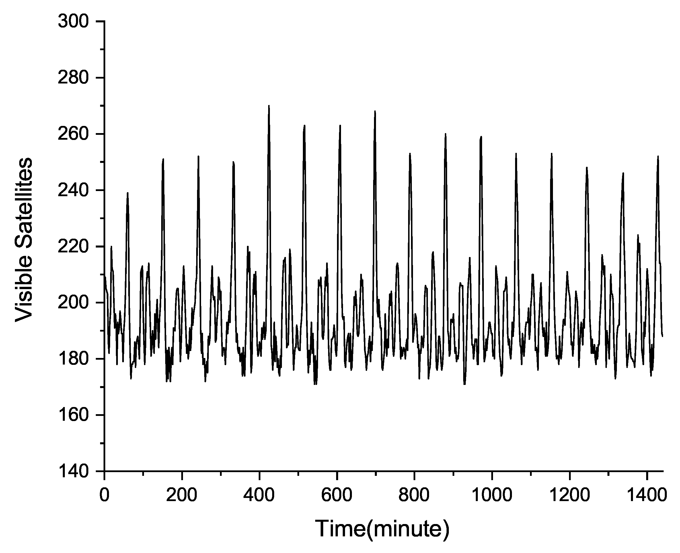
Time (hour)	Maximum Number of Satellites Observed per Hour	Maximum Number of Satellites Observed per Hour (with Random Obstruction)
1	239	195
2	232	201
3	251	208
4	232	187
5	252	218
6	250	213
7	220	190
8	270	227
9	263	212
10	214	183
11	263	218
12	268	234
13	214	181
14	253	217
15	260	215
16	216	183
17	259	219
18	253	216
19	210	177
20	253	215
21	248	210
22	217	183
23	246	208
24	252	201

, with the support of a sufficiently large number of LEO satellites under observing conditions, the GDOP of the final localization is lower than 0.3 in order of magnitude, but in the real environment, localizing all observable satellites greatly increases the computational complexity. At the same time, it also imposes an unnecessary burden on the satellite network and reduces the algorithm’s real-time performance. Therefore, it is important to choose the most suitable satellites for a receiver with high accuracy. Therefore, selecting as many satellites as possible within a suitable range for a receiver with high accuracy has high engineering significance.

In order to evaluate the performance of the proposed satellite selection algorithm, we set up a comparative trial with the recursive algorithm, a Quasi-Optimal algorithm, and the algorithm proposed in this study.

As described in Section 2.2, the recursive algorithm takes the variation of the GDOP (which is in a way similar to the slope of a specific satellite) as the influence value of each satellite and retains the few satellites with the highest influence values to construct the final satellite selection result. The Quasi-Optimal algorithm employs an approximate geometric leveling selection strategy. In the trial, the final combination size of the satellites was fixed at 10 to 80 in intervals of 10. The GDOP results of the three algorithms were compared. An Intel(R) Core(TM) i5-8500 CPU @ 3.00 GHz with 16 GB of RAM was used as the simulation hardware for a computation load comparison.

Table 3. Time consumed by each algorithm in the trial.

Algorithm	Consumed Time (s)
Quasi_Optimal Algorithm	$4.323\times {10}^{-3}$
Recursive Algorithm	10.326 (form 200 to 10)
Proposed Algorithm	0.132

shows the time consumed by each algorithm during a single satellite selection.

Figure 4 and

Table 4. Average GDOP per day of different satellite sizes constructed by each algorithm under random obstruction or without obstruction.

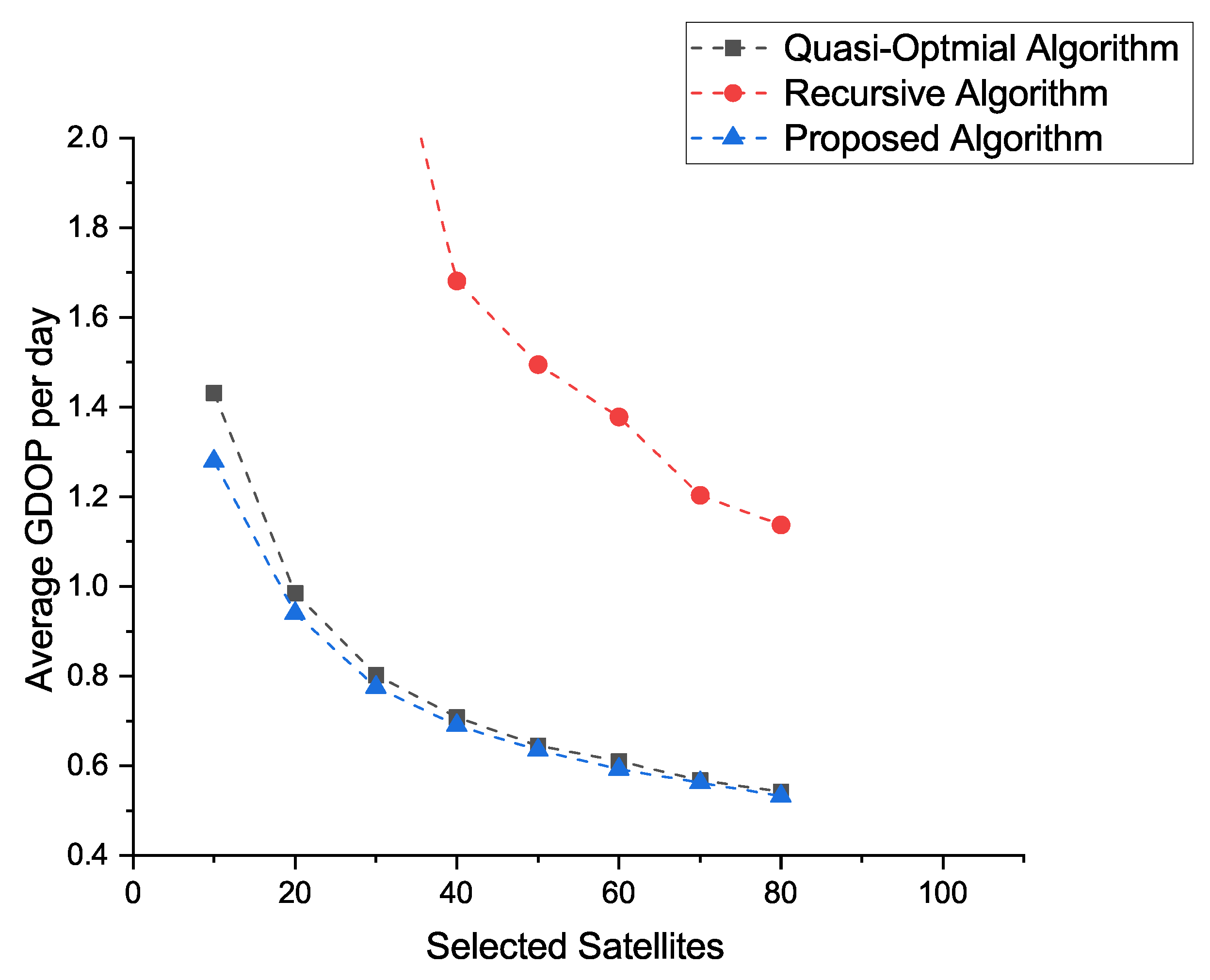
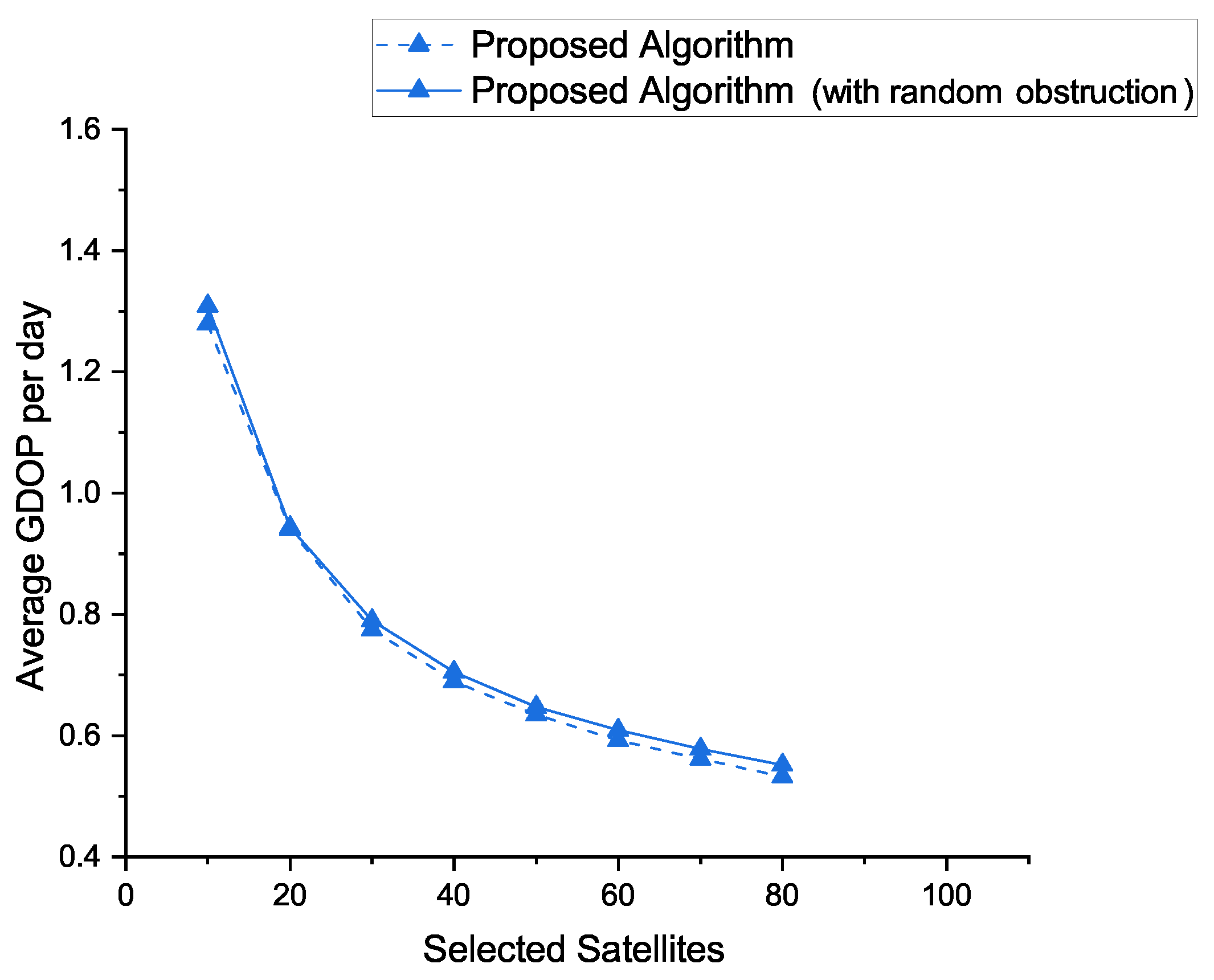
Satellites	Quasi_Optimal Algorithm	Recursive Algorithm	Proposed Algorithm	Quasi_Optimal Algorithm (with Random Obstruction)	Recursive Algorithm (with Random Obstruction)	Proposed Algorithm (with Random Obstruction)
10	1.431	1855.158	1.279	1.882	782.354	1.308
20	0.985	32.339	0.940	1.082	9.481	0.943
30	0.802	2.398	0.775	0.919	1.848	0.790
40	0.708	1.682	0.690	0.800	1.516	0.705
50	0.645	1.495	0.634	0.735	1.340	0.647
60	0.610	1.378	0.592	0.690	1.176	0.609
70	0.567	1.203	0.562	0.649	1.066	0.578
80	0.542	1.137	0.532	0.625	0.923	0.551

show that the recursive algorithm has a better performance in the case of observation constraints. It performs better under observation constraints because it is difficult for it to evaluate the impact of each satellite on localization when excluding many of them, and it erroneously excludes important ones during the process. However, this also means that it cannot be well applied when selecting a small number of satellites out of a large number for localization. Therefore, its application should be limited to scenarios where the number of observable satellites is close to that of the number to be selected.

As shown in Figure 5, in the unobstructed environment, the proposed algorithm has a similar performance to the Quasi-Optimal algorithm, which has no significant advantage. Except for the case of selecting 10 satellites, the daily average GDOP difference of the proposed algorithm with the Quasi-Optimal algorithm is below 0.05. Meanwhile, the Quasi-Optimal algorithm is based on purely geometric positional computation, which is much more computationally efficient, so the proposed algorithm does not have a significant advantage under unobstructed conditions.

Figure 6 shows the significant increase in the average GDOP when using the Quasi-Optimal algorithm based on randomly 60°-azimuthal satellites occluded by obstructions. The daily average GDOP difference decreases as the number of satellites increases, which shows a clear performance impact. For example, the difference is around 0.08 with 60–80 satellites, around 0.10 with 20–50 satellites, and 0.45 with 10 satellites with fewer observations. This indicates that obstruction has a significant impact on the performance of current classical geometric satellite selection algorithms, which implies limitations in engineering applications.

Figure 7 shows a comparison of the performance of the proposed algorithm in an occluded and an open field. If there are no obstructions, the proposed algorithm is effective for overcoming the limitation that some of the satellites cannot be observed due to environmental signal blocking. There is basically no big difference between the average daily GDOP of the two conditions, which shows that they have similar performance under unobstructed conditions. However, the average daily GDOP difference for different numbers of satellites varies: It is only 0.02 for most cases, except for the 10-satellite case where the difference is 0.03. However, there is a situation in which the daily average GDOP is higher in an unoccluded environment than in an occluded environment; this is probably due to the fact that the genetic algorithm used is not specially optimized for this problem, and the local convergence phenomenon affects the final results.

As shown in Figure 8, the proposed algorithm improves the performance of GDOP in an occluded environment. The average daily GDOP difference is 0.57 with 10 satellites, 0.14 with 20 satellites, 0.13 with 30 satellites, around 0.09 with 40–60 satellites, and around 0.07 with 70–80 satellites. Based on these results, it can be concluded that the proposed algorithm can effectively improve the localization accuracy under a single large-angle obstruction.

4.2. Random 240° Obstruction Simulations-Multiple Small-Angle Obstructions

To compare the performance of the two algorithms more effectively, we conducted an experiment of occluding a 240° angle. We divided the horizon into 36 regions with a 10° azimuth angle each and randomly removed the visible satellites in 24 regions. We then applied the Quasi-Optimal algorithm and the proposed algorithm to the remaining satellites, and present the results in Figure 9 and

Table 5. The effect of obstruction at a 240° angle on the maximum number of visible satellites per hour. GDOP values when selecting 10 satellites using the Quasi-Optimal algorithm and the proposed algorithm.

Time (hour)	Maximum Visible Satellites per Hour	10 Satellites GDOP (Proposed Algorithnm)	10 Satellites GDOP (Quasi-Optimal Algorithm)
1	98	1.249	1.432
2	80	1.252	1.423
3	74	1.293	2.422
4	63	1.373	2.625
5	86	1.252	1.522
6	93	1.321	1.351
7	74	1.242	1.660
8	88	1.224	1.720
9	91	1.231	1.485
10	72	1.274	1.523
11	85	1.165	1.432
12	95	1.329	1.829
13	77	1.351	1.774
14	89	1.293	1.388
15	96	1.353	1.531
16	64	1.340	1.461
17	86	1.285	2.044
18	77	1.306	1.555
19	71	1.274	1.389
20	74	1.435	1.539
21	79	1.417	2.243
22	72	1.262	1.884
23	80	1.323	1.782
24	92	1.177	1.279

.

Figure 9 shows the case of selecting 10 satellites after applying the algorithm with a 240° obstruction. The GDOP difference of both algorithms is lower than 0.3 after 12 h; this is due to the fact that multiple small-angle obstruction more easily take a uniform distribution with respect to a single large-angle obstruction, so the satellites are more likely to take a uniform distribution. The daily average GDOP difference when selecting 10 satellites is 0.386, which is lower than that of the case of a single large-angle occluded case; however, the proposed algorithm shows a higher stability in the case of multiple small-angle obstructions.

5. Conclusions

The significant increase of visible LEO satellites not only improves positioning accuracy, but also poses a challenge to low-cost receivers. In this study, we derived the optimal configuration of positioning satellites and transformed it into an optimization problem, which we solved with a genetic algorithm. We verified the performance advantages of our algorithm by simulating data from Starlink satellites in orbit.

The following conclusions can be drawn from the static and low-dynamic single-epoch positioning results of the Quasi-Optimal algorithm, the recursive algorithm, and the proposed algorithm:

(a)

The recursive algorithm cannot be well applied when selecting a small number of satellites out of a large number for localization. Therefore, its application is more appropriate in scenarios where the number of observable satellites is close to that of the number to be selected.

(b)

Obstruction has a significant impact on the performance of current classical geometric satellite selection algorithms, such as the Quasi-Optimal algorithm, which limits engineering applications.

(c)

The proposed algorithm can overcome the limitation that some of the satellites cannot be observed due to obstructions.

(d)

It is easier to obtain a uniform distribution for multiple small-angle obstructions compared with a single large-angle obstruction, which makes the performance difference between the Quasi-Optimal algorithm and the proposed algorithm smaller than when there is a single large-angle obstruction, but the proposed algorithm still has a higher stability.

In the future, the addition of visible satellites in commercial large-scale LEO satellite constellations will increase the accuracy of localization and enhance the positioning ability under obstructions. This will render the proposed algorithm even more advantageous. Key areas for further research include optimizing the parameters of the genetic algorithm to avoid falling into local optima and improving the algorithm’s computational speed.

References

- Phatak, M. Recursive method for optimum GPS satellite selection. IEEE Trans. Aerosp. Electron. Syst. 2001, 37, 751–754. [Google Scholar] [CrossRef]
- Liu, M.; Fortin, M.A.; Landry, R., Jr. A Recursive Quasi-optimal Fast Satellite Selection Method for GNSS Receivers. In Proceedings of the 22nd International Technical Meeting of the Satellite Division of the Institute of Navigation (Ion Gnss 2009), Savannah, GA, USA, 22–25 September 2009; pp. 2061–2071. [Google Scholar]
- Li, G.; Xu, C.; Zhang, P.; Hu, C. A Modified Satellite Selection Algorithm Based on Satellite Contribution for GDOP in GNSS. In Lecture Notes in Electrical Engineering; Springer: Berlin/Heidelberg, Germany, 2012; Volume 176, pp. 415–421. [Google Scholar] [CrossRef]
- Teng, Y.; Wang, J. New Characteristics of Geometric Dilution of Precision (GDOP) for Multi-GNSS Constellations. J. Navig. 2014, 67, 1018–1028. [Google Scholar] [CrossRef]
- Ou, G.; Li, G.; Peng, A. Fast satellite selection method for multi-constellation Global Navigation Satellite System under obstacle environments. IET Radar Sonar Navig. 2014, 8, 1051–1058. [Google Scholar] [CrossRef]
- Nie, Z.; Gao, Y.; Wang, Z.; Ji, S. A new method for satellite selection with controllable weighted PDOP threshold. Surv. Rev. 2017, 49, 285–293. [Google Scholar] [CrossRef]
- Zhang, P. Research on satellite selection algorithm in ship positioning based on both geometry and geometric dilution of precision contribution. Int. J. Adv. Robot. Syst. 2019, 16, 172988141983024. [Google Scholar] [CrossRef]
- Abedi, A.A.; Mosavi, M.R.; Mohammadi, K. A new recursive satellite selection method for multi-constellation GNSS. Surv. Rev. 2020, 52, 330–340. [Google Scholar] [CrossRef]
- Shi, J.; Li, K.; Chai, L.; Liang, L.; Tian, C.; Xu, K. Fast satellite selection algorithm for GNSS multi-system based on Sherman–Morrison formula. GPS Solut. 2023, 27, 44. [Google Scholar] [CrossRef]
- Park, C.W.; How, J.P. Quasi-Optimal Satellite Selection Algorithm for Real-Time Applications. In Proceedings of the 14th International Technical Meeting of the Satellite Division of The Institute of Navigation (ION GPS 2001), Salt Lake City, UT, USA, 11–14 September 2001; pp. 3018–3028. [Google Scholar]
- Zheng, Z.-y.; Huang, C.; Feng, C.-g.; Zhang, F.-p. Selection of GPS satellites for the optimum geometry. Chin. Astron. Astrophys. 2004, 28, 80–87. [Google Scholar] [CrossRef]
- Zhang, M.; Zhang, J. A Fast Satellite Selection Algorithm: Beyond Four Satellites. IEEE J. Sel. Top. Signal Process. 2009, 3, 740–747. [Google Scholar] [CrossRef]
- Li, F.; Li, Z.; Gao, J.; Yao, Y. A Fast Rotating Partition Satellite Selection Algorithm Based on Equal Distribution of Sky. J. Navig. 2019, 72, 1053–1069. [Google Scholar] [CrossRef]
- Yang, L.; Gao, J.; Li, Z.; Li, F.; Chen, C.; Wang, Y. New Satellite Selection Approach for GPS/BDS/GLONASS Kinematic Precise Point Positioning. Appl. Sci. 2019, 9, 5280. [Google Scholar] [CrossRef]
- Jang, J.; Park, D.; Sung, S.; Lee, Y.J. HDOP and VDOP Analysis in an Ideal Placement Environment for Dual GNSSs. Sensors 2022, 22, 3475. [Google Scholar] [CrossRef]
- Teng, Y.; Wang, J. A closed-form formula to calculate geometric dilution of precision (GDOP) for multi-GNSS constellations. GPS Solut. 2016, 20, 331–339. [Google Scholar] [CrossRef]
- Meng, F.; Wang, S.; Zhu, B. Research of Fast Satellite Selection Algorithm for Multi-constellation. Chin. J. Electron. 2016, 25, 1172–1178. [Google Scholar] [CrossRef]
- Blanco-Delgado, N.; Duarte Nunes, F.; Seco-Granados, G. On the relation between GDOP and the volume described by the user-to-satellite unit vectors for GNSS positioning. GPS Solut. 2017, 21, 1139–1147. [Google Scholar] [CrossRef]
- Verma, P.; Hajra, K.; Banerjee, P.; Bose, A. Evaluating PDOP in Multi-GNSS Environment. IETE J. Res. 2019, 68, 1705–1712. [Google Scholar] [CrossRef]
- Xue, S.; Yang, Y. Positioning configurations with the lowest GDOP and their classification. J. Geod. 2015, 89, 49–71. [Google Scholar] [CrossRef]
- Teng, Y.; Wang, J.; Huang, Q. Mathematical minimum of Geometric Dilution of Precision (GDOP) for dual-GNSS constellations. Adv. Space Res. 2016, 57, 183–188. [Google Scholar] [CrossRef]
- Xue, S.; Yang, Y. Understanding GDOP minimization in GNSS positioning: Infinite solutions, finite solutions and no solution. Adv. Space Res. 2017, 59, 775–785. [Google Scholar] [CrossRef]
- Song, J.; Xue, G.; Kang, Y. A Novel Method for Optimum Global Positioning System Satellite Selection Based on a Modified Genetic Algorithm. PLoS ONE 2016, 11, e0150005. [Google Scholar] [CrossRef]
- Huang, P.; Rizos, C.; Roberts, C. Satellite selection with an end-to-end deep learning network. GPS Solut. 2018, 22, 108. [Google Scholar] [CrossRef]
- Singh, P.; Joshi, J.; Dey, A.; Sharma, N. GNSS Satellite Selection-based on Per-satellite Parameters Using Deep Learning. IETE J. Res. 2022, 1–12. [Google Scholar] [CrossRef]
- Wang, E.; Sun, C.; Wang, C.; Qu, P.; Huang, Y.; Pang, T. A satellite selection algorithm based on adaptive simulated annealing particle swarm optimization for the BeiDou Navigation Satellite System/Global Positioning System receiver. Int. J. Distrib. Sens. Netw. 2021, 17, 155014772110317. [Google Scholar] [CrossRef]
- Guan, X.; Chai, H.; Xiao, G.; Han, J.; Han, S.; Shufeng, M. A fast satellite selection algorithm for multi-GNSS marine positioning based on improved particle swarm optimisation. Surv. Rev. 2021, 54, 554–565. [Google Scholar] [CrossRef]
- Zhao, D.; Cai, C.; Li, L. A binary discrete particle swarm optimization satellite selection algorithm with a queen informant for Multi-GNSS continuous positioning. Adv. Space Res. 2021, 68, 3521–3530. [Google Scholar] [CrossRef]
- Biswas, S.K. Unsupervised learning-based satellite selection algorithm for GPS–NavIC multi-constellation receivers. GPS Solut. 2022, 26, 61. [Google Scholar] [CrossRef]
- Luo, S.; Wang, L.; Tu, R.; Zhang, W.; Wei, J.; Chen, C. Satellite selection methods for multi-constellation advanced RAIM. Adv. Space Res. 2020, 65, 1503–1517. [Google Scholar] [CrossRef]
- Wang, H.; Cheng, Y.; Cheng, C.; Li, S.; Li, Z. Research on Satellite Selection Strategy for Receiver Autonomous Integrity Monitoring Applications. Remote Sens. 2021, 13, 1725. [Google Scholar] [CrossRef]
- Zhao, W.; Duan, L.; Jian, X. A Satellite Selection Strategy of SURF IA in Airport Intelligent Monitoring. Math. Probl. Eng. 2022, 2022, 8966814. [Google Scholar] [CrossRef]
- Rajasekhar, C.; Srilatha Indira Dutt, V.; Sasibhushana Rao, G. Weighted GDoP for improved position accuracy using NavIC and GPS hybrid constellation over Indian sub-continent. Int. J. Intell. Netw. 2021, 2, 42–45. [Google Scholar] [CrossRef]
- Du, H.; Hong, Y.; Xia, N.; Zhang, G.; Yu, Y.; Zhang, J. A Navigation Satellites Selection Method Based on ACO with Polarized Feedback. IEEE Access 2020, 8, 168246–168261. [Google Scholar] [CrossRef]
- Xia, N.; Zhi, Q.; He, M.; Hong, Y.; Du, H. A navigation satellite selection algorithm for optimized positioning based on Gibbs sampler. Int. J. Distrib. Sens. Netw. 2020, 16, 155014772092962. [Google Scholar] [CrossRef]
- Liu, X.; Zhang, S.; Zhang, Q.; Zheng, N.; Zhang, W.; Ding, N. A novel partial ambiguity resolution based on ambiguity dilution of precision- and convex-hull-based satellite selection for instantaneous multiple global navigation satellite systems positioning. J. Navig. 2022, 75, 832–848. [Google Scholar] [CrossRef]
- Yoshida, S. Study on Cloud-Based GNSS Positioning Architecture with Satellite Selection Algorithm and Report of Field Experiments. IEICE Trans. Commun. 2022, 105, 388–398. [Google Scholar] [CrossRef]
- Niu, X.; Dai, Y.; Liu, T.; Chen, Q.; Zhang, Q. Feature-based GNSS positioning error consistency optimization for GNSS/INS integrated system. GPS Solut. 2023, 27, 89. [Google Scholar] [CrossRef]
- Misra, P.; Enge, P. Global Positioning System: Signals, Measurements, and Performance, 2nd ed.; Ganga-Jamuna Press: Lincoln, MA, USA, 2012; pp. 199–232. [Google Scholar]
- Wei, M.; Liu, Z.; Li, C.; Yang, R.; Li, B.; Xu, Q. A Combined Satellite Selection Algorithm. In Proceedings of the 2018 International Conference on Security, Pattern Analysis, and Cybernetics (SPAC), Jinan, China, 14–17 December 2018; pp. 477–480. [Google Scholar] [CrossRef]