Simulation of Thermal Infrared Brightness Temperatures from an Ocean Color and Temperature Scanner Onboard a New Generation Chinese Ocean Color Observation Satellite

Abstract

Since 2002, China has launched four Haiyang-1 (HY-1) satellites equipped with the Chinese Ocean Color and Temperature Scanner (COCTS), which can observe the sea surface temperature (SST). The planned new generation ocean color observation satellites also carry a sensor for observing the SST represented by the payload in this paper. We analyze the spectral brightness temperature (BT) difference between the payload and the Moderate Resolution Imaging Spectroradiometer (MODIS) onboard Terra for the thermal infrared channels (11 and 12 µm) based on atmospheric radiative transfer simulation. The bias and standard deviation (SD) of spectral BT difference for the 11 µm channel are −0.12 K and 0.15 K, respectively, and those for the 12 µm channel are −0.10 K and 0.03 K, respectively. When the total column water vapor (TCWV) decreases from the oceans near the equator to high-latitude oceans, the spectral BT difference of the 11 µm channel varies from a positive deviation to a negative deviation, and that of the 12 µm channel basically remains stable. By correcting the MODIS BT observation using the spectral BT differences, we produce the simulated BT data for the thermal infrared channels of the payload, and then validate it using the Infrared Atmospheric Sounding Interferometer (IASI) carried on METOP-B. The validation results show that the bias of BT difference between the payload and IASI is −0.22 K for the 11 µm channel, while it is −0.05 K for the 12 µm channel. The SD of both channels is 0.13 K. In this study, we provide the simulated BT dataset for the 11 and 12 µm channels of a payload for the retrieval of SST. The simulated BT dataset corrected may be used to develop SST-retrieval algorithms.

1. Introduction

Haiyang-1 (HY-1) satellites are the first generation of China’s ocean color series satellites. HY-1A was the first experimental satellite, launched on 15 May 2002. HY-1B was the successor of HY-1A and was launched on 11 April 2007. HY-1C was the first operational satellite, launched on 7 September 2018. HY-1D was designed to perform complementary observations with HY-1C in the morning and afternoon and was launched on 11 June 2020. Both HY-1A and HY-1B are in orbit at a height of 798 km and a tilting angle of 98.8°. A descending node local time of HY-1A is 8:53–10:10 a.m. and that of HY-1B is about 10:30 a.m. Both HY-1C and HY-1D are in orbit at a height of 782 km and a tilting angle of 98.5°. A descending node local time of HY-1C is approximately at 10:30 a.m. and that of HY-1D is about at 1:30 a.m. All four satellites are equipped with the Chinese Ocean Color and Temperature Scanner (COCTS) capable of observing the sea surface temperature (SST). The ground pixel resolution of the COCTS is approximately 1.1 km, with a swath width of about 2900 km. The COCTS is a ten-band sensor, including eight visible bands and two thermal infrared bands with the center wavelengths about 11 and 12 µm, respectively.

The new generation ocean color observation satellite is planned to be launched, and it will also carry a sensor for observing the SST represented by the payload in this paper. The payload still includes two thermal infrared channels at 11 and 12 µm. For pre-researching the SST-retrieval algorithm, the brightness temperature (BT) data of these two channels are essential. Generally, the physical properties and performance characteristics of the sensor are determined through a series of comprehensive and systematic tests before launch, as well as the calibration algorithm before launch and in orbit [1,2,3,4]. In the absence of pre-launch test data, and under the premise that the spectral characteristics of the two thermal infrared channels of the payload are close to the corresponding channels (M15 and M16) of the Suomi National Polar-orbiting Partnership (S-NPP)/Visible Infrared Imaging Radiometer (VIIRS) satellite, we created a simulated BT dataset for the 11 and 12 µm channels of the payload and provided the test data for pre-research of the SST-retrieval algorithm. In this study, we conduct BT simulation research using the spectral response functions (SRFs) of the S-NPP/VIIRS instead of the payload.

Considering that the 11 and 12 µm channels of the Terra/Moderate Resolution Imaging Spectroradiometer (MODIS) have shown a stable long-term trend [5], and with continuous updates in calibration and algorithm improvements, it has resolved issues encountered during on-orbit operation and currently provides high-quality data products [6]. Therefore, based on atmospheric radiative transfer simulation, we corrected the MODIS BT observation using the spectral BT differences between the payload and MODIS, and created a simulated BT dataset for the thermal infrared channels of the payload. In Section 2, an overview of the datasets is provided. Section 3 describes the method of the BT simulation. Section 4 presents the results, including the analysis of spectral BT differences and creation of a simulated BT dataset. Section 5 evaluates the simulated BT. Section 6 concludes the study.

2. Datasets

The datasets consist of Terra/MODIS data products, METOP-B/Infrared Atmospheric Sounding Interferometer (IASI) data, and the fifth generation of global atmospheric reanalysis products (ERA5) distributed by the European Centre for Medium-Range Weather Forecasts (ECMWF). In this study the time of the datasets used were the 1st, 8th, 15th, and 22nd of each month in 2019. The spatial coverage was global oceans.

2.1. Terra/MODIS Data

Terra was successfully launched in December 1999. The orbit altitude is 705 km, and the tilting angle is 98.5°. The local time at the descending node is 10:30 a.m. MODIS onboard Terra achieves a swath width of 2330 km with a scanning pattern of ±55°. It provides global coverage every one to two days. MODIS has 36 spectral channels. The spectrum ranges from 0.4 to 14.4 µm [7].

In this study, the MODIS data products used include MOD021KM, MOD03, and MOD35_L2 [8,9,10]. All are 5-min granule, and the spatial resolution is 1 km. The data format is HDF. The MOD021KM data product contains calibrated radiances and solar reflectance for all bands. The MOD03 data product contains geolocation information, such as longitude, latitude, satellite zenith angle (SZA), land–water mask, etc. The MOD35_L2 contains a cloud mask and quality assurance for the cloud mask, etc. These three MODIS data products are versioned as Collection 6.1.

2.2. METOP-B/IASI Spectral Radiance Data

METOP-B is a polar satellite launched in September 2012. Its orbital altitude is 827 km and the tilting angle is 98.7°. The local time at the descending node is 9:30 a.m. [11]. IASI onboard METOP-B is used for measuring the infrared atmospheric spectra. IASI consists of a Fourier Transform Spectrometer and an Infrared Imager. The spectral range of IASI is from 3.62 µm to 15.5 µm, and a spectral sampling resolution of that is 0.25 cm⁻¹, which results in 8461 spectral samples [12].

In this study, we use the radiance data from the EUMETSAT Polar System (EPS) IASI Level 1C data product. The data product is accessed in EPS native format [13]. The data contain longitude, latitude, time, spectral radiance, wavenumber, SZA, etc. [14].

2.3. ECMWF ERA5 Data

ERA5 data products are distributed by ECMWF. In this study, we use ERA5 hourly data on pressure levels and on single levels, regridded to a 0.25° latitude–longitude grid. The data are accessed in NetCDF. The vertical resolution of ERA5 hourly data on pressure levels is 37 pressure levels, and the main variables include geopotential, atmospheric temperature, relative humidity, ozone mass mixing ratio, wind, etc. The main variables of the ERA5 hourly data on single levels include 2 m temperature of air, skin temperature, 10 m wind, total column water vapor (TCWV), etc. [15].

3. Methods

3.1. Data Preprocessing

We used the flag information from the cloud mask data provided by the MOD35_L2 product to select daytime and nighttime clear-sky ocean pixels, respectively. Since ERA5 data are used for the atmospheric radiative transfer simulation, the radiance data and the SZA of the selected ocean pixels from the MOD021KM product were projected onto a latitude–longitude grid of 0.25° × 0.25°, the same as the spatial resolution of ERA5 data using the geolocation information from the MOD03 product. Figure 1a,b show the MODIS 11 and 12 µm BT images on 15 January 2019.

For the ocean pixels selected, longitude, latitude, skin temperature, and horizontal and vertical wind-speed components were extracted from the ERA5 surface parameter product. The longitude, latitude, geopotential, ozone mixing ratio, relative humidity, specific humidity, and atmospheric temperature profiles are also extracted from the ERA5 atmospheric parameter product. In order to show the demos of MODTRAN profiles, a position is randomly selected in the tropical, midlatitude, and subarctic regions, respectively. Figure 2, Figure 3 and Figure 4 show, in turn, examples of atmospheric temperature profiles, zone profiles, and specific humidity profiles for simulation on the three positions. Subgraphs a–d in Figure 2, Figure 3 and Figure 4, respectively, represent the profiles at 22:00 on 1 January, 1 April, 1 July, and 1 October 2019.

3.2. Simulation of Atmospheric Infrared Radiative Transfer

The MODerate resolution atmospheric TRANsmission (MODTRAN) model, developed by Spectral Sciences Incorporated and the Air Force Research Laboratory, is a tool used to solve the radiative transfer equation using a narrow-band method. It simulates the process of radiance passing through the Earth’s atmosphere. The input file for MODTRAN is an ASCII format file consisting of a series of formatted cards (CARDS). CARD1, CARD1A, CARD2, CARD3, CARD4, and CARD5 are the six mandatory cards that must be input. They define the model’s algorithm type, scattering model, atmospheric profile input parameters, aerosols and clouds, observation geometry, spectral range and resolution, and program loop settings, respectively. MODTRAN can simulate physical quantities such as atmospheric transmittance, radiance, and BT at the top of the atmosphere.

3.3. BT Simulation of Ocean Color and Temperature Scanner

The simulated BT of the payload is obtained by correcting the observed BT of MODIS using the spectral BT difference between the payload and MODIS. Figure 5 shows the flowchart of the simulated BT process for the payload.

According to the flowchart in Figure 5, for the selected ocean pixels we simulate the 11 and 12 µm BT of the payload and MODIS, respectively. The input of MODTRAN simulation includes SZA, ERA5 surface parameters, ERA5 atmospheric parameters, and the spectral response function. By calculating the BT difference simulated by MODTRAN between the payload and MODIS for each channel, the observed BT of the two thermal infrared channels of MODIS is corrected. Finally, the 11 and 12 µm simulated BT dataset of the payload are created.

4. Results

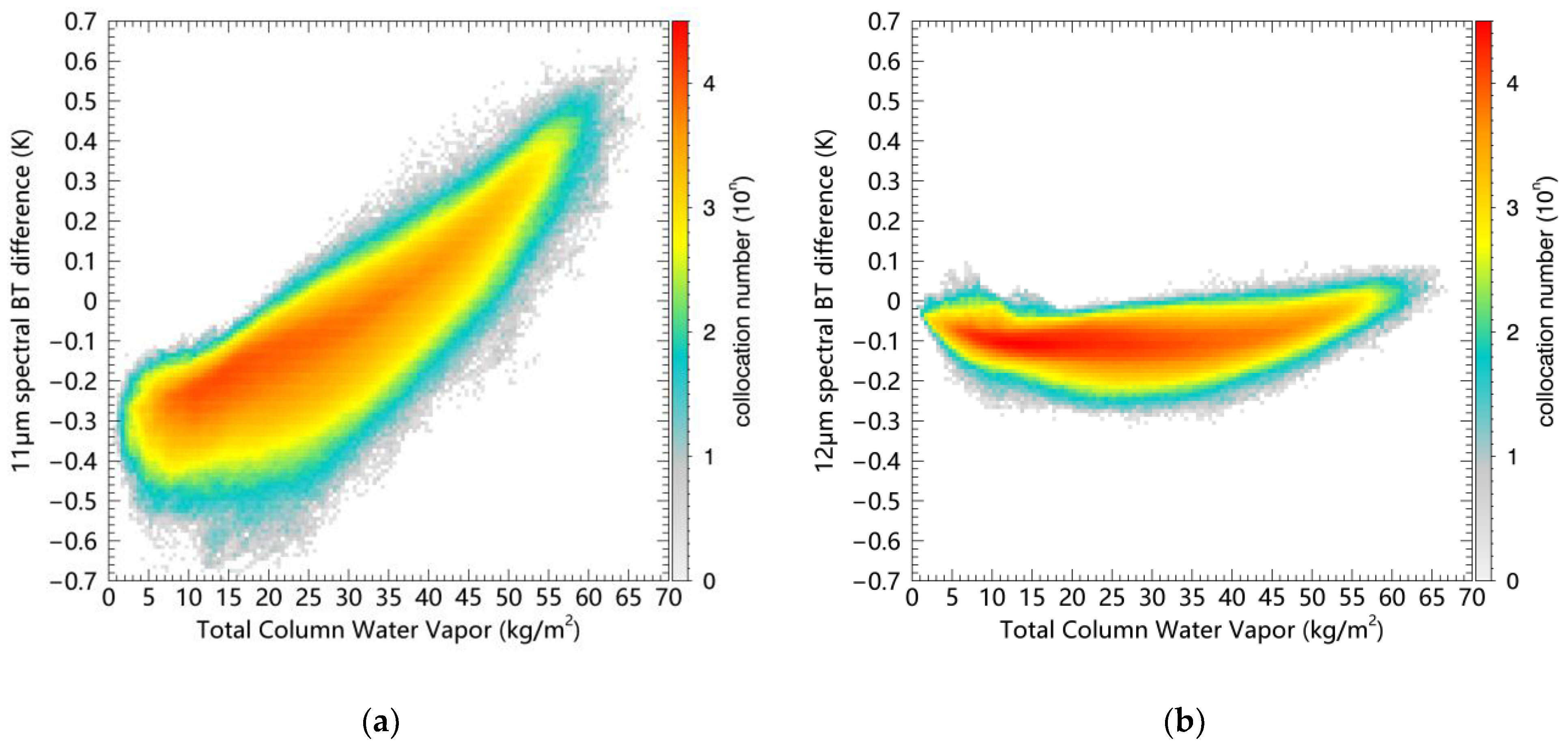
4.1. Spectral BT Difference

By comparing the MODTRAN profiles between the payload and MODIS, we know that only the spectral response functions are different. So, the spectral differences can be quantitatively characterized using atmospheric radiative transfer simulations with MODTRAN. Figure 6 and Figure 7 display the scatter plots of the payload BT against MODIS BT simulated by MODTRAN for the 11 and 12 µm channels, respectively. Figure 6a and Figure 7a show the scatter plots during the day, and Figure 6b and Figure 7b show scatter plots at night. The collocation number in an interval of 0.25 K BT is indicated by the color. The scattered points in the 11 µm channel deviate more from the diagonal line than the 12 µm channel. Figure 8 and Figure 9 display the histogram of the differences of BT simulated by MODTRAN between the payload and MODIS in the 11 and 12 µm channels, respectively. The interval of the BT difference is 0.025 K (Figure 8a and Figure 9a show daytime results and Figure 8b and Figure 9b show nighttime results). It can also be clearly seen that the BT differences in the 11 µm channel are concentrated between −0.6 K and 0.6 K, while the BT differences in the 12 µm channel are concentrated between −0.3 K and 0 K. The dynamic range of the 11 µm BT differences is wider. With regard to statistics, the bias and standard deviation (SD) of the 11 µm BT differences are −0.12 K and 0.15 K, respectively, while those of the 12 µm BT differences are −0.10 K and 0.03 K, respectively.

The global and latitudinal distribution characteristics of spectral BT differences between the payload and MODIS were analyzed. Figure 10 and Figure 11 show the global and latitudinal distribution of the BT differences in the 11 µm channel, respectively. Figure 12 and Figure 13 show the global and latitudinal distribution of the BT differences in the 12 µm channel, respectively. Figure 10a, Figure 11a, Figure 12a and Figure 13a represent daytime results and Figure 10b, Figure 11b, Figure 12b and Figure 13b represent nighttime results.

According to Figure 10 and Figure 11, the spectral BT differences between the payload and MODIS in the 11 µm channel exhibit the highest positive deviation near the equator. As the latitude moves from the equator toward the North and South poles, the spectral BT differences first decrease and then increase, eventually presenting a negative deviation. The maximum positive deviation in the latitudinal direction is about 0.16 K and occurs around 5°N. The maximum negative deviation is about −0.28 K. In the Northern Hemisphere, this occurs around 60°N, and in the Southern Hemisphere, it occurs around 55°S. In Figure 12 and Figure 13, spectral BT differences between the payload and MODIS at the 12 µm channel exhibit an overall negative deviation. The maximum negative deviation is around 35°N and 35°S. In the Northern Hemisphere, as the latitude moves from around 35°N toward the North Pole or the equator, the latitudinal spectral BT differences decrease gradually. Similar variation trends can also be observed in the Southern Hemisphere. The latitudinal spectral BT differences vary from −0.12 K to 0 K.

Next, we analyzed the relationship of the spectral BT differences and TCWV. The TCWV data are extracted from the ERA5 hourly data on single levels. Figure 14 shows the global distribution of TCWV. By comparing Figure 10 with Figure 14, it can be seen that the 11 µm spectral BT differences show negative deviation in the lower TCWV regions and positive deviation in the higher TCWV regions. By comparing Figure 12 with Figure 14, we know that TCWV has little effect on the 12 µm spectral BT differences. Figure 15a,b shows the variations of the 11 and 12 µm spectral BT differences with TCWV, respectively. The 11 µm BT differences are relatively larger in lower and higher TCWV regions and vary from a negative deviation to positive deviation with increasing TCWV. The 12 µm BT differences basically remain stable with increasing TCWV.

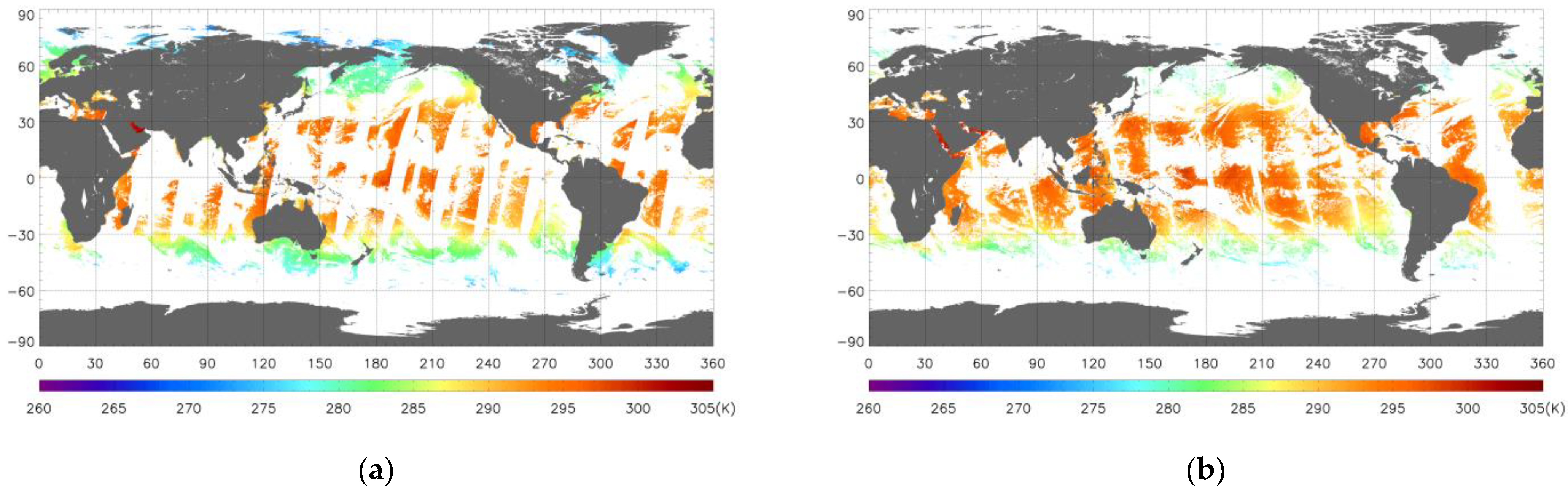
4.2. Simulated BT of the Payload

The simulated BT of the payload was produced by correcting the MODIS BT observed using the spectral BT differences between the payload and MODIS. The expression that represents the relationship among the simulated BT of the payload, MODIS BT observation, and the spectral BT differences is Equation (1), where ${BT}_{simulated}$ represents the simulated BT of the payload, ${BT}_{MODIS}$ represents the MODIS BT observation, and $∆{BT}_{spectral}$ represents the spectral BT differences. As the spatial resolution of $∆{BT}_{spectral}$ is 0.25°, not equal to the spatial resolution of ${BT}_{MODIS}$, $∆{BT}_{spectral}$ needs to be interpolated to the same spatial resolution as ${BT}_{MODIS}$.

$${BT}_{simulated}={BT}_{MODIS}+∆{BT}_{spectral}$$

(1)

We created the 11 and 12 µm simulated BT dataset of the payload, respectively. There are 13,802 files in the dataset of each channel. We took the 11 and 12 µm simulated BT images of the payload on 22 September 2019 as an example, as shown in Figure 16 and Figure 17 (Figure 16a and Figure 17a show daytime results and Figure 16b and Figure 17b show nighttime results).

5. Discussion

To retrieve SST from infrared remote sensing, the 11 and 12 µm BTs are essential parameters. The accuracy of the BTs will affect the quality of SST inversion. In order to evaluate the accuracy of the 11 and 12 µm simulated BTs of the payload, we selected the METOP-B/IASI as the reference sensor. IASI is selected by the Global Space-based Inter-Calibration System (GSICS) as a reference sensor [16]. IASI has a high spectral resolution and accurate and stable calibration accuracy and orbit stability. It was calibrated using the observations of internal black bodies and cold space [17,18]. Before launch, it was calibrated and corrected by comparison with an external large area reference blackbody (HBB) [18,19]. After launch, IASI data were routinely monitored and validated to ensure the characterization of IASI [17]. In addition, IASI on the METOP series satellites also has the advantage of long-term data continuity. Figure 18 shows the curves of the BTs measured by IASI between 9 µm and 13.5 µm, and the two simulated spectral response curves of the payload.

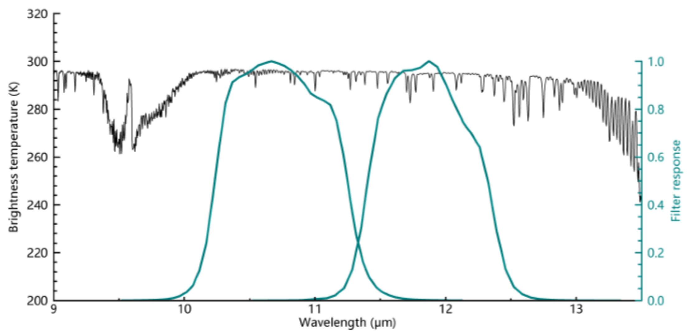
5.1. IASI Convolution BT

The IASI data include the radiance for 8461 channels every 0.25 cm⁻¹. Using Equation (2), we calculate the IASI-convolved radiance by convolving the IASI radiance with the SRFs of the simulated channels of the payload [20].

$$R_i=\frac{{\int }_a^{b}R\left(\lambda \right)F_i\left(\lambda \right)d\lambda }{{\int }_a^b{F}_i\left(\lambda \right)d\lambda }$$

(2)

where i is the channel number, $R\left(\lambda \right)$ is the IASI radiance, $F_i\left(\lambda \right)$ is the payload spectral response function, $R_i$ is the IASI-convolved radiance, and $a$ and $b$ are the initial value and final value of the payload in wavelength.

This convolution process yields the IASI-convolved radiance of the two simulated payload channels. Using the radiance and BT look-up table based on the Planck equation, the IASI-convolved radiance is converted to BT. Figure 19 shows the IASI daytime and nighttime BT images for the 11 µm channel on 8 May 2019.

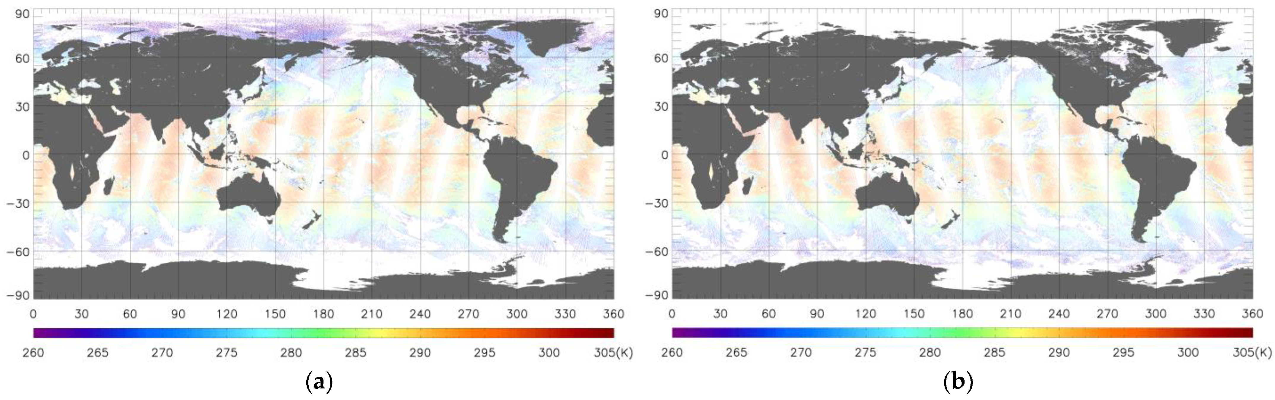
5.2. Validation of the Simulated BT

To validate the simulated BT of the payload for the 11 and 12 µm channels, we referred the IASI BT. Considering that the simulated BT of the payload are in a 5-min granule, and the spatial resolution of the payload and the IASI are 1 km and 12 km, respectively, we project the payload and IASI BT on a 0.12° latitude–longitude grid in a 30-min temporal window. The BT of the payload clear-sky ocean pixels located in a grid within the temporal window is evenly averaged, and the number is represented by the count. For the impact caused by the different atmospheric path, we diminish it by setting the absolute value of the SZAs secant difference to be less than 0.03 [21,22]. By analyzing the variations in the payload minus IASI BT against the count shown in Figure 20 (Figure 20a shows the 11 µm result and Figure 20b shows the 12 µm result) and against the maximum minus minimum BT of the payload in a grid shown in Figure 21 (Figure 21a is 11 µm and Figure 21b is 12 µm), we can see that most of the matchups distribute in areas where the count is greater than 50 and the maximum minus minimum BT is less than 0.6 K. The color in Figure 20 represents the collocation number in an interval of 1 for count and 0.01 K for the BT difference between the payload and IASI. In Figure 21, the color represents the collocation number in an interval of 0.01 K payload BT maximum minus minimum and 0.01 K difference between the payload and IASI BT. Because the IASI BT does not perform clear-sky data screening and the payload BT is an average of clear-sky ocean pixels in the projection grid, abnormal matchups exist in these areas. Thus, after filtering the matchups by setting the count as 50, and setting the payload BT maximum minus minimum as 0.6 K in the projection grid, we eliminated the matchups wherein the BT difference between the payload and IASI is more than three times the robust standard deviation (RSD) from the median. Figure 22 and Figure 23 show the histograms of the validation matchups between the payload and IASI BT for the 11 and 12 µm channels, respectively. Figure 22a and Figure 23a show daytime results, and Figure 22b and Figure 23b show nighttime results. The interval of the BT difference is 0.05 K. After statistical analysis, the bias and SD of the 11 µm BT difference between the payload and IASI are −0.22 K and 0.13 K, respectively, and those of the 12µm BT difference are −0.05 K and 0.13 K, respectively.

6. Conclusions

Based on the atmospheric radiative transfer simulation, we analyzed the spectral BT differences between a payload and MODIS. The bias and SD of the 11 µm BT differences are −0.12 K and 0.15 K, respectively, while those of the 12 µm BT differences are −0.10 K and 0.03 K, respectively. The 11 µm spectral BT differences are more affected by TCWV than the 12 µm channel. In high-latitude oceans, TCWV is lower, and the BT differences of the payload minus MODIS show a negative deviation. In oceans near the equator, TCWV is higher, and the BT differences between the payload and MODIS show a positive deviation. Meanwhile, the 12 µm channel BT differences of the payload minus MODIS basically remain stable with increasing TCWV. Utilizing the spectral BT differences, the MODIS BT observation was corrected, and the simulated BT dataset for the thermal infrared channels of the payload were created and validated using IASI as the reference. The results show that the bias and SD of the 11 µm BT difference between the payload and IASI are −0.22 K and 0.13 K, respectively, and those of the 12 µm BT difference are −0.05 K and 0.13 K, respectively. In this study, we provide the 11 and 12 µm simulated BT dataset of a payload for the retrieval of SST. The simulated BT dataset corrected may be used to develop of SST-retrieval algorithms.

References

1. Barnes, W.L.; Pagano, T.S.; Salomonson, V.V. Prelaunch Characteristics of the Moderate Resolution Imaging Spectroradiometer (MODIS) on EOS-AM1. IEEE Trans. Geosci. Remote Sens. 1998, 36, 1088–1100. [Google Scholar] [CrossRef]
2. Oudrari, H.; McIntire, J.; Xiong, X.; Butler, J.; Lee, S.; Lei, N.; Schwarting, T.; Sun, J. Prelaunch Radiometric Characterization and Calibration of the S-NPP VIIRS Sensor. IEEE Trans. Geosci. Remote Sens. 2015, 53, 2195–2210. [Google Scholar] [CrossRef]
3. Oudrari, H.; McIntire, J.; Xiong, X.; Butler, J.; Ji, Q.; Schwarting, T.; Lee, S.; Efremova, B. JPSS-1 VIIRS Radiometric Characterization and Calibration Based on Pre-launch Testing. Remote Sens. 2016, 8, 41. [Google Scholar] [CrossRef]
4. Mcintire, J.; Moyer, D.; Oudrari, H.; Xiong, X. Pre-launch Radiometric Characterization of JPSS-1 VIIRS Thermal Emissive Bands. Remote Sens. 2016, 8, 47. [Google Scholar] [CrossRef]
5. Chang, T.; Xiong, X.; Shrestha, A. Assessment of MODIS Thermal Emissive Bands Calibration Performance Using Deep Convective Clouds. J. Appl. Remote Sens. 2019, 13, 44526. [Google Scholar] [CrossRef]
6. Xiong, X.; Angal, A.; Chang, T.; Chiang, K.; Lei, N.; Li, Y.; Sun, J.; Twedt, K.; Wu, A. MODIS and VIIRS Calibration and Characterization in Support of Producing Long-Term High-Quality Data Products. Remote Sens. 2020, 12, 3167. [Google Scholar] [CrossRef]
7. Barnes, W.L.; Xiong, X.; Salomonson, V.V. Status of Terra MODIS and Aqua MODIS. Adv. Space Res. 2003, 32, 2099–2106. [Google Scholar] [CrossRef]
8. MODIS Level 1B Product User’s Guide. 2012. Available online: https://mcst.gsfc.nasa.gov/sites/default/files/file_attachments/M1054D_PUG_083112_final.pdf (accessed on 28 August 2020).
9. MODIS Geolocation Fields Product. 2017. Available online: https://ladsweb.modaps.eosdis.nasa.gov/missions-and-measurements/products/MOD03 (accessed on 13 August 2020).
10. MODIS Atmosphere L2 Cloud Mask Product. 2015. Available online: https://ladsweb.modaps.eosdis.nasa.gov/missions-and-measurements/products/MOD35_L2 (accessed on 13 August 2020).
11. Klaes, K.D.; Holmlund, K. EUMETSAT Programmes and Plans. In Proceedings of the SPIE Optical Engineering + Applications, San Diego, CA, USA, 17–21 August 2014; Proceedings Volume 9218. Earth Observing Systems XIX, 92181D. [Google Scholar] [CrossRef]
12. Simeoni, D.; Astruc, P.; Miras, D.; Alis, C.; Andreis, O.; Scheidel, D.; Degrelle, C.; Nicol, P.; Bailly, B.; Guiard, P.; et al. Design and Development of IASI Instrument. In Proceedings of the Optical Science and Technology, The SPIE 49th Annual Meeting, Denver, CO, USA, 2–6 August 2004; Proceedings Volume 5543. Infrared Spaceborne Remote Sensing XII. [Google Scholar] [CrossRef]
13. Generic Product Format Specification. 2010. Available online: http://eodg.atm.ox.ac.uk/user/dudhia/iasi/documents/PDF_TEN_96167-EPS-GPFS.pdf (accessed on 13 February 2022).
14. IASI Level 1: Product Guide. 2019. Available online: https://www-cdn.eumetsat.int/files/2020-04/pdf_iasi_pg.pdf (accessed on 17 October 2021).
15. Hersbach, H.; Bell, B.; Berrisford, P.; Hirahara, S.; Horányi, A.; Muñoz-Sabater, J.; Nicolas, J.; Peubey, C.; Radu, R.; Schepers, D.; et al. The ERA5 Global Reanalysis. Q. J. R. Meteorol. Soc. 2020, 146, 1999–2049. [Google Scholar] [CrossRef]
16. Chander, G.; Hewison, T.J.; Fox, N.; Wu, X.; Xiong, X.; Blackwell, W.J. Overview of Intercalibration of Satellite Instruments. IEEE Trans. Geosci. Remote Sens. 2013, 51, 1056–1080. [Google Scholar] [CrossRef]
17. Hilton, F.; Armante, R.; August, T.; Barnet, C.; Bouchard, A.; Camy-Peyret, C.; Capelle, V.; Clarisse, L.; Clerbaux, C.; Coheur, P.-F.; et al. Hyperspectral Earth Observation from IASI: Five Years of Accomplishments. Bull. Am. Meteorol. Soc. 2012, 93, 347–370. [Google Scholar] [CrossRef]
18. Blumstein, D.; Chalon, G.; Carlier, T.; Buil, C.; Hebert, P.; Maciaszek, T.; Ponce, G.; Phulpin, T.; Tournier, B.; Simeoni, D.; et al. IASI Instrument: Technical Overview and Measured Performances. In Proceedings of the Optical Science and Technology, The SPIE 49th Annual Meeting, Denver, CO, USA, 2–6 August 2004; Proceedings Volume 5543. Infrared Spaceborne Remote Sensing XII. [Google Scholar] [CrossRef]
19. GSICS Traceability Statement for IASI and AIRS. 2014. Available online: https://www-cdn.eumetsat.int/files/2020-04/pdf_trace_stat_iasi_airs.pdf (accessed on 13 July 2023).
20. Liu, M. Retrieval of Infrared and Microwave Sea Surface Temperature from HY-1B and HY-2A Satellite Observations. Ph.D. Thesis, Ocean University of China, Qingdao, China, 2019. [Google Scholar]
21. Liu, M.; Merchant, C.J.; Guan, L.; Mittaz, J.P.D. Inter-Calibration of HY-1B/COCTS Thermal Infrared Channels with MetOp-A/IASI. Remote Sens. 2018, 10, 1173. [Google Scholar] [CrossRef]
22. Liu, M.; Guan, L.; Liu, J.; Song, Q.; Ma, C.; Li, N. First Assessment of HY-1C COCTS Thermal Infrared Calibration Using MetOp-B IASI. Remote Sens. 2021, 13, 635. [Google Scholar] [CrossRef]
Figure 1. (a) The MODIS 11 µm BT, (b) the MODIS 12 µm BT for one granule on 15 January 2019.
Remotesensing 15 05059 g001
Figure 2. The atmospheric temperature profiles at 22:00 on (a) 1 January, (b) 1 April, (c) 1 July, and (d) 1 October 2019.
Remotesensing 15 05059 g002
Figure 3. The ozone profiles at 22:00 on (a) 1 January, (b) 1 April, (c) 1 July, and (d) 1 October 2019.
Remotesensing 15 05059 g003
Figure 4. The specific humidity profiles at 22:00 on (a) 1 January, (b) 1 April, (c) 1 July, and (d) 1 October 2019.
Remotesensing 15 05059 g004
Figure 5. The flowchart of the simulated BT process for the payload.
Remotesensing 15 05059 g005
Figure 6. The scatter plots of the payload BT against MODIS BT simulated by MODTRAN in the 11 µm channel: (a) during the day; (b) at night.
Remotesensing 15 05059 g006
Figure 7. The scatter plots of the payload BT against MODIS BT simulated by MODTRAN in the 12 µm channel: (a) during the day; (b) at night.
Remotesensing 15 05059 g007
Figure 8. The histogram of the differences of BT simulated by MODTRAN between the payload and MODIS in the 11 µm channel: (a) during the day; (b) at night.
Remotesensing 15 05059 g008
Figure 9. The histogram of the differences of BT simulated by MODTRAN between the payload and MODIS in the 12 µm channel: (a) during the day; (b) at night.
Remotesensing 15 05059 g009
Figure 10. The global distribution characteristics of spectral BT differences between the payload and MODIS in 11 µm channel: (a) during the day; (b) at night.
Remotesensing 15 05059 g010
Figure 11. The latitudinal distribution characteristics of spectral BT differences between the payload and MODIS in 11 µm channel: (a) during the day; (b) at night.
Remotesensing 15 05059 g011
Figure 12. The global distribution characteristics of spectral BT differences between the payload and MODIS in 12 µm channel: (a) during the day; (b) at night.
Remotesensing 15 05059 g012
Figure 13. The latitudinal distribution characteristics of spectral BT differences between the payload and MODIS in 12 µm channel: (a) during the day; (b) at night.
Remotesensing 15 05059 g013
Figure 14. The global distribution map of TCWV.
Remotesensing 15 05059 g014
Figure 15. The variations of: (a) the 11 µm spectral BT differences; (b) the 12 µm spectral BT differences with TCWV.
Remotesensing 15 05059 g015
Figure 16. The simulated BT images of the payload for the 11 µm channel on 22 September 2019: (a) during the day; (b) at night.
Remotesensing 15 05059 g016
Figure 17. The simulated BT images of the payload for the 12 µm channel on 22 September 2019: (a) during the day; (b) at night.
Remotesensing 15 05059 g017
Figure 18. Example of IASI spectrum (black curve) between 9 µm and 13.5 µm expressed in brightness temperature (K) and the SRFs (teal curve) of the simulated channels of the payload.
Remotesensing 15 05059 g018
Figure 19. The IASI BT images for 11 µm channel on 8 May 2019: (a) daytime; (b) nighttime.
Remotesensing 15 05059 g019
Figure 20. The variations in the BT difference between the payload and IASI against count in a grid: (a) 11 µm; (b) 12 µm.
Remotesensing 15 05059 g020
Figure 21. The variations in the BT difference between the payload and IASI against the maximum minus minimum BT of the payload in a grid: (a) 11 µm; (b) 12 µm.
Remotesensing 15 05059 g021
Figure 22. The histograms of the matchups between the payload and IASI 11 µm BT: (a) during the day; (b) at night.
Remotesensing 15 05059 g022
Figure 23. The histograms of the matchups between the payload and IASI 12 µm BT: (a) during the day; (b) at night.
Remotesensing 15 05059 g023
Disclaimer/Publisher’s Note: The statements, opinions and data contained in all publications are solely those of the individual author(s) and contributor(s) and not of MDPI and/or the editor(s). MDPI and/or the editor(s) disclaim responsibility for any injury to people or property resulting from any ideas, methods, instructions or products referred to in the content.