
Polar Sea Ice Detection Using a Rotating Fan Beam Scatterometer

Abstract
:
1. Introduction
2. CSCAT on CFOSAT
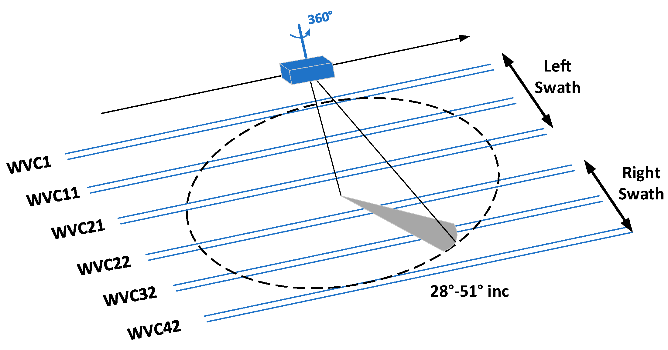
2.1. Geometry of Observation
2.2. Scientific Product Specification of CSCAT
- (1)
- L1B data include the time ordered slices σ0 and slice geolocations.
- (2)
- L2A data include the average backscatter value of each WVC (usually with a resolution of 25 km), and each WVC obtains 2–8 views of each antenna beam.
- (3)
- L2B data include the sea surface wind information.
3. Sea Ice Detection Algorithm of CSCAT
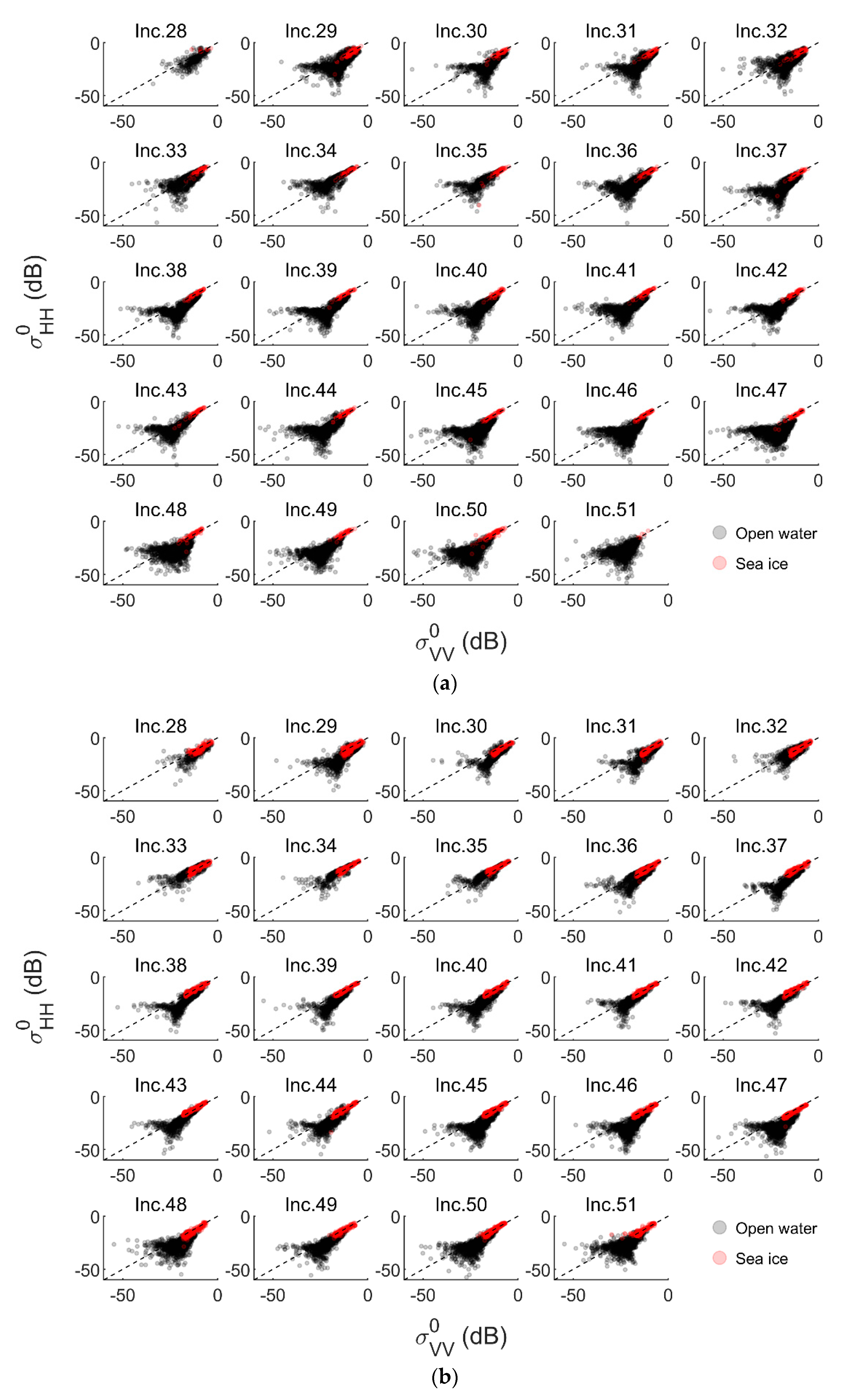
3.1. CSCAT Backscatter Space
3.2. GMF for Sea Ice
3.3. Backscatter Distances to Sea Ice GMF
3.4. Squared Distances to GMFs
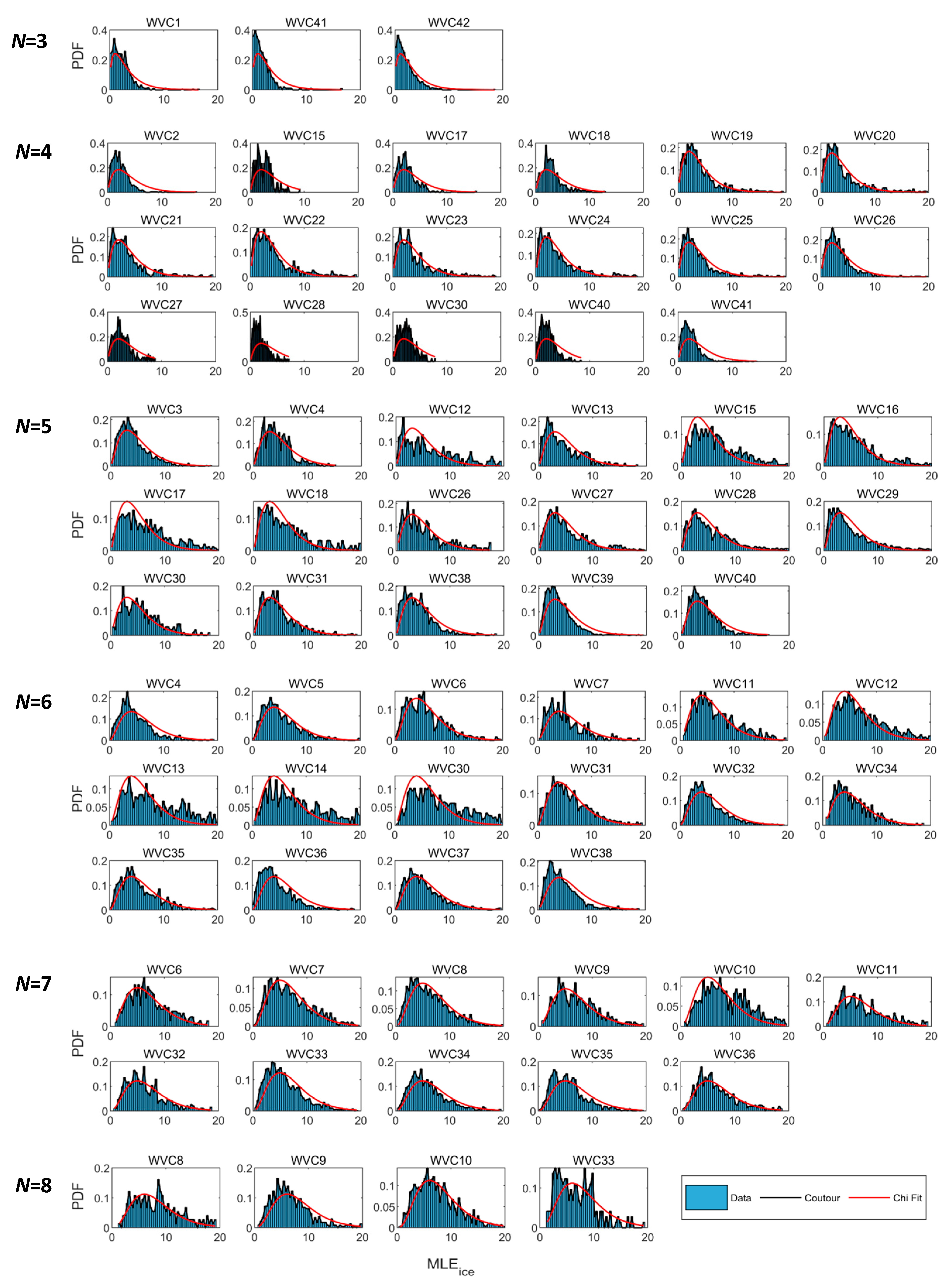
3.4.1. MLEice
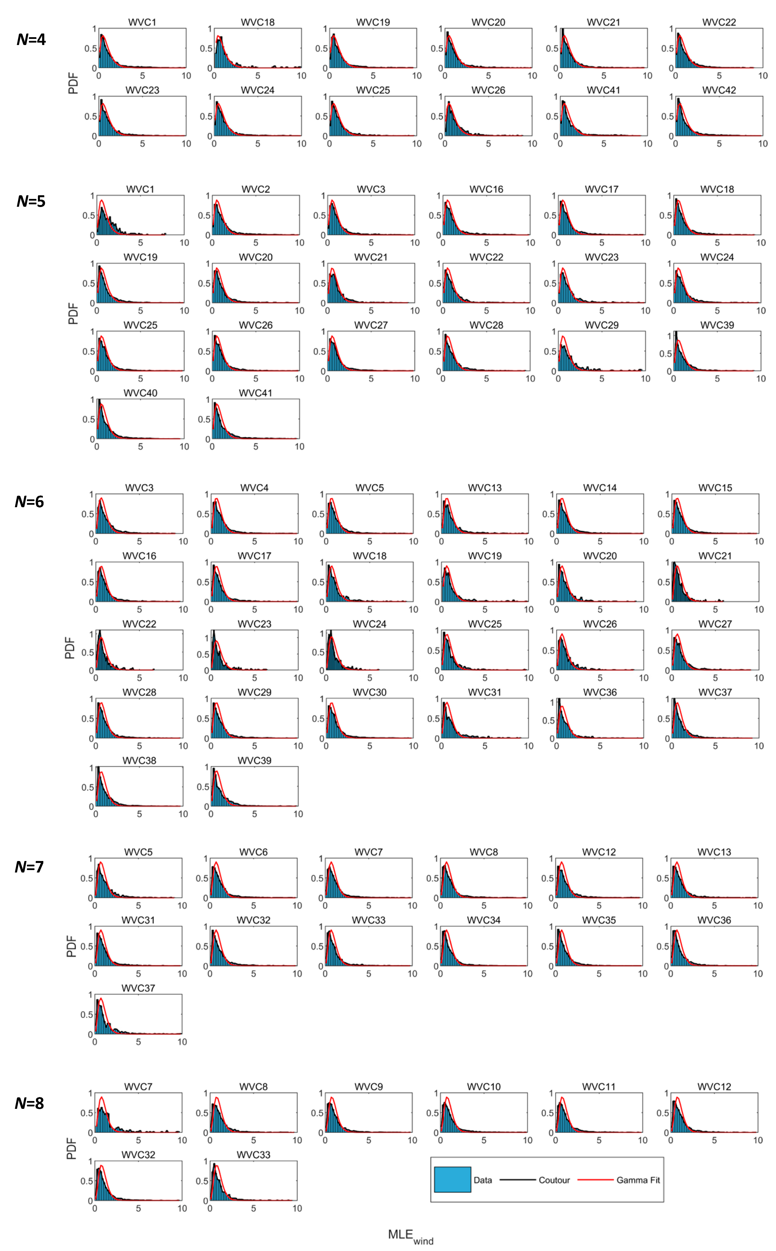
3.4.2. MLEwind
3.5. Bayesian Posterior Probabilities of Sea Ice
4. Results and Discussion
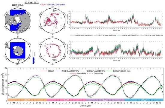
4.1. Sea Ice Mapping
4.2. Validation
4.2.1. Validation Sources
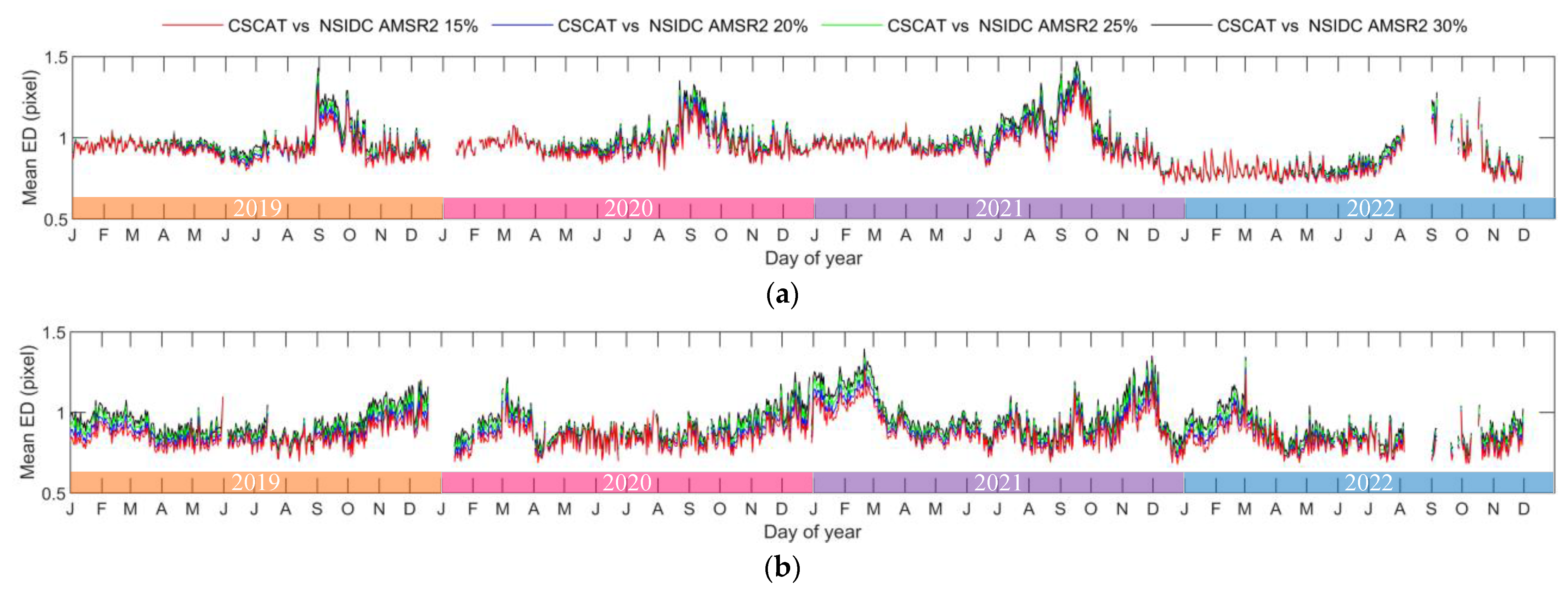
4.2.2. Sea Ice Edge Comparison
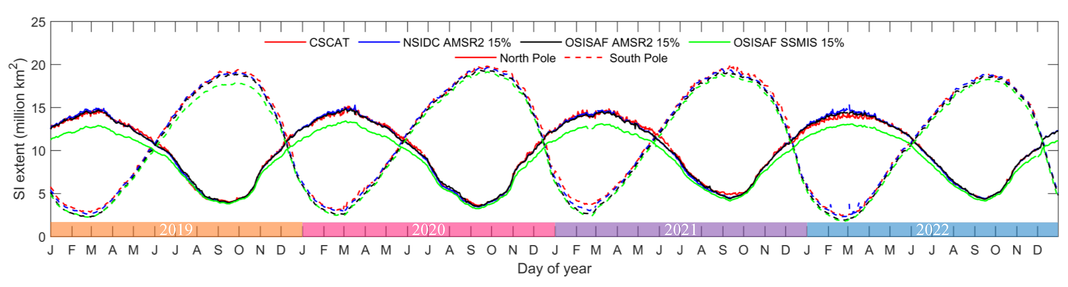
4.2.3. Sea Ice Extent Comparison
5. Conclusions
Author Contributions
Funding
Data Availability Statement
Acknowledgments
Conflicts of Interest
References
- Long, D.G. Polar Applications of Spaceborne Scatterometers. IEEE J. Sel. Top. Appl. Earth Obs. Remote Sens. 2017, 10, 2307–2320. [Google Scholar] [CrossRef] [PubMed]
- Singh, S.; Tiwari, R.K.; Sood, V.; Kaur, R.; Prashar, S. The Legacy of Scatterometers: Review of applications and perspective. IEEE Geosci. Remote Sens. Mag. 2022, 10, 39–65. [Google Scholar] [CrossRef]
- Verspeek, J. Sea Ice Classification Using Bayesian Statistics; KNMI: De Bilt, The Netherlands, 2006. [Google Scholar]
- Liu, J.; Lin, W.; Dong, X.; Lang, S.; Yun, R.; Zhu, D.; Zhang, K.; Sun, C.; Mu, B.; Ma, J.; et al. First Results From the Rotating Fan Beam Scatterometer Onboard CFOSAT. IEEE Trans. Geosci. Remote Sens. 2020, 58, 8793–8806. [Google Scholar] [CrossRef]
- Daily Arctic and Antarctic Sea Ice Extents and Normalized Backscatter. Available online: https://scatterometer.knmi.nl/ice_extents/ (accessed on 7 August 2023).
- Li, Z.; Verhoef, A.; Stoffelen, A.; Shang, J.; Dou, F. First Results from the WindRAD Scatterometer on Board FY-3E: Data Analysis, Calibration and Wind Retrieval Evaluation. Remote Sens. 2023, 15, 2087. [Google Scholar] [CrossRef]
- Zhai, X.; Wang, Z.; Zheng, Z.; Xu, R.; Dou, F.; Xu, N.; Zhang, X. Sea Ice Monitoring with CFOSAT Scatterometer Measurements Using Random Forest Classifier. Remote Sens. 2021, 13, 4686. [Google Scholar] [CrossRef]
- Xu, C.; Wang, Z.; Zhai, X.; Lin, W.; He, Y. SVM-Based Sea Ice Extent Retrieval Using Multisource Scatterometer Measurements. Remote Sens. 2023, 15, 1630. [Google Scholar] [CrossRef]
- Remund, Q.P.; Long, D.G. Sea ice extent mapping using Ku band scatterometer data. J. Geophys. Res. Ocean. 1999, 104, 11515–11527. [Google Scholar] [CrossRef]
- Anderson, H.; Long, D.G. Sea ice mapping method for SeaWinds. IEEE Trans. Geosci. Remote Sens. 2005, 43, 647–657. [Google Scholar] [CrossRef]
- Near Real-Time Sea Ice Discrimination Using SeaWinds on QUIKSCAT. Available online: https://cdn.knmi.nl/system/data_center_publications/files/000/068/084/original/sea_ice_osi_saf_final_report.pdf?1495621021 (accessed on 7 August 2023).
- Rivas, M.B.; Stoffelen, A. New Bayesian Algorithm for Sea Ice Detection with QuikSCAT. IEEE Trans. Geosci. Remote Sens. 2011, 49, 1894–1901. [Google Scholar] [CrossRef]
- Rivas, M.B.; Verspeek, J.; Verhoef, A.; Stoffelen, A. Bayesian Sea Ice Detection with the Advanced Scatterometer ASCAT. IEEE Trans. Geosci. Remote Sens. 2012, 50, 2649–2657. [Google Scholar] [CrossRef]
- Otosaka, I.; Rivas, M.B.; Stoffelen, A. Bayesian Sea Ice Detection with the ERS Scatterometer and Sea Ice Backscatter Model at C-Band. IEEE Trans. Geosci. Remote Sens. 2018, 56, 2248–2254. [Google Scholar] [CrossRef]
- Liu, L.; Dong, X.; Lin, W.; Lang, S.; Wang, L. Polar Sea Ice Detection with the CFOSAT Scatterometer. In Proceedings of the IEEE International Geoscience and Remote Sensing Symposium, Brussels, Belgium, 11–16 July 2021. [Google Scholar]
- Liu, L.; Zhai, H.; Dong, X.; Zhao, F. SEA ICE Extent Retrieval with Ku-Band Rotating Fan Beam Scatterometer Data. In Proceedings of the IEEE International Geoscience and Remote Sensing Symposium, Kuala Lumpur, Malaysia, 17–22 July 2022. [Google Scholar]
- Li, Z.; Verhoef, A.; Stoffelen, A. Bayesian Sea Ice Detection Algorithm for CFOSAT. Remote Sens. 2022, 14, 3569. [Google Scholar] [CrossRef]
- Lin, W.; Dong, X.; Portabella, M.; Lang, S.; He, Y.; Yun, R.; Wang, Z.; Xu, X.; Zhu, D.; Liu, J. A Perspective on the Performance of the CFOSAT Rotating Fan-Beam Scatterometer. IEEE Trans. Geosci. Remote Sens. 2018, 57, 627–639. [Google Scholar] [CrossRef]
- Yun, R.; Dong, X.; Liu, J.; Lin, W.; Zhu, D.; Ma, J.; Lang, S.; Wang, Z. CFOSAT Rotating Fan-beam Scatterometer Backscatter Measurement Processing. Earth Space Sci. 2021, 8, 1–18. [Google Scholar] [CrossRef]
- A Guide to NSIDC’s Polar Stereographic Projection, National Snow and Ice Data Center. Available online: https://nsidc.org/data/user-resources/help-center/guide-nsidcs-polar-stereographic-projection (accessed on 7 August 2023).
- Sandven, S.; Spreen, G.; Heygster, G.; Girard-Ardhuin, F.; Farrell, S.; Dierking, W.; Allard, R. Sea Ice Remote Sensing—Recent Developments in Methods and Climate Data Sets. Surv. Geophys. 2023, 44, 1–37. [Google Scholar] [CrossRef]
- Markus, T.; Cavalieri, D.J. An enhancement of the NASA Team sea ice algorithm. IEEE Trans. Geosci. Remote Sens. 2000, 38, 1387–1398. [Google Scholar] [CrossRef]
- Markus, T.; Cavalieri, D.J. The AMSR-E NT2 Sea Ice Concentration Algorithm: Its Basis and Implementation. J. Remote Sens. Soc. Jpn. 2009, 29, 216–225. [Google Scholar] [CrossRef]
- AMSR-E/AMSR2 Unified L3 Daily 12.5 km Brightness Temperatures, Sea Ice Concentration, Motion & Snow Depth Polar Grids V001. Version 1. Available online: https://catalog.data.gov/dataset/amsr-e-amsr2-unified-l3-daily-12-5-km-brightness-temperatures-sea-ice-concentration-motion (accessed on 7 August 2023).
- OSI SAF Global Sea Ice Concentration (SSMIS), OSI-401-d. Available online: https://osi-saf.eumetsat.int/products/osi-401-d (accessed on 7 August 2023).
- OSI SAF Global Sea Ice Concentration (AMSR-2), OSI-408-a. Available online: https://osi-saf.eumetsat.int/products/osi-408-a (accessed on 7 August 2023).
- Contour-to-Contour Distance. Available online: https://www.mathworks.com/matlabcentral/fileexchange/75551-contour-to-contour-distance (accessed on 7 August 2023).


| Incidence | 2019 | 2020 | 2021 | 2022 | ||||
|---|---|---|---|---|---|---|---|---|
| Bias | Std | Bias | Std | Bias | Std | Bias | Std | |
| 30° | 0.11 | 1.46 | 0.10 | 1.59 | 0.17 | 1.86 | 0.14 | 1.91 |
| 31° | 0.12 | 1.40 | 0.09 | 1.49 | 0.04 | 1.72 | 0.21 | 1.79 |
| 32° | −0.06 | 1.34 | −0.02 | 1.56 | −0.10 | 1.86 | 0.11 | 1.84 |
| 33° | −0.05 | 1.32 | 0.01 | 1.57 | −0.05 | 1.97 | 0.06 | 1.78 |
| 34° | 0.06 | 1.32 | 0.11 | 1.60 | 0.25 | 2.02 | 0.24 | 1.84 |
| 35° | 0.07 | 1.25 | 0.09 | 1.55 | 0.20 | 1.97 | 0.19 | 1.8 |
| 36° | 0.04 | 1.20 | 0.02 | 1.59 | −0.09 | 1.98 | 0.03 | 1.77 |
| 37° | −0.02 | 1.12 | −0.12 | 1.42 | −0.16 | 1.68 | −0.07 | 1.58 |
| 38° | −0.03 | 0.99 | −0.13 | 1.17 | −0.21 | 1.34 | −0.19 | 1.34 |
| 39° | 0.16 | 0.98 | −0.05 | 1.05 | −0.16 | 1.23 | −0.07 | 1.24 |
| 40° | −0.02 | 0.95 | −0.17 | 0.99 | −0.28 | 1.15 | −0.15 | 1.21 |
| 41° | −0.07 | 0.96 | −0.06 | 1.07 | −0.20 | 1.26 | −0.02 | 1.24 |
| 42° | 0.03 | 0.99 | −0.06 | 1.10 | 0.06 | 1.33 | 0.12 | 1.23 |
| 43° | −0.03 | 0.97 | −0.14 | 0.99 | −0.09 | 1.20 | 0.01 | 1.17 |
| 44° | −0.19 | 1.02 | −0.28 | 0.92 | −0.19 | 1.17 | −0.16 | 1.19 |
| 45° | −0.14 | 1.03 | −0.23 | 0.77 | −0.32 | 1.02 | −0.27 | 1.1 |
| 46° | 0.04 | 1.02 | 0.04 | 0.71 | −0.04 | 0.90 | −0.16 | 1.03 |
| 47° | −0.06 | 1.10 | 0.01 | 0.68 | −0.08 | 0.83 | 0.16 | 0.97 |
| 48° | 0.08 | 1.17 | 0.02 | 0.74 | 0.04 | 0.89 | 0.16 | 1.07 |
| 49° | 0.22 | 1.21 | −0.01 | 0.75 | 0.14 | 0.93 | 0.20 | 1.04 |
| N | 4 | 5 | 6 | 7 | 8 |
|---|---|---|---|---|---|
| 2019 | 0.45 | 0.35 | 0.30 | 0.25 | 0.23 |
| 2020 | 0.36 | 0.28 | 0.24 | 0.20 | 0.18 |
| 2021 | 0.45 | 0.35 | 0.30 | 0.27 | 0.25 |
| 2022 | 0.99 | 0.77 | 0.66 | 0.55 | 0.51 |
| Data Source | Sensor | Temporal Coverage | Temporal Sampling | Spatial Coverage | Spatial Sampling |
|---|---|---|---|---|---|
| NOAA NSIDC | SSMIS | January 2015 to present | 1 per day | Global | 25 km |
| AMSRE | June 2002 to October 2011 | 1 per day | Global | 12.5 km | |
| AMSR2 | July 2012 to present | 1 per day | Global | 12.5 km | |
| EUMETSAT OSI SAF | SSMIS | March 2005 to present | 1 per day | Global | 10 km |
| AMSR2 | September 2016 to present | 1 per day | Global | 10 km |
| Region | Comparisons | Sea Ice Concentration Threshold | Absolute Mean (106 km2) | Standard Deviation (106 km2) | ||||||
|---|---|---|---|---|---|---|---|---|---|---|
| 2019 | 2020 | 2021 | 2022 | 2019 | 2020 | 2021 | 2022 | |||
| North Pole | CSCAT vs. NSIDC AMSR2 | 15% | 0.02 | 0.06 | 0.16 | 0.17 | 0.68 | 0.22 | 0.24 | 0.31 |
| 20% | 0.03 | 0.11 | 0.21 | 0.11 | 0.68 | 0.22 | 0.25 | 0.30 | ||
| 25% | 0.08 | 0.16 | 0.27 | 0.06 | 0.68 | 0.22 | 0.25 | 0.30 | ||
| 30% | 0.12 | 0.21 | 0.31 | 0.01 | 0.68 | 0.22 | 0.25 | 0.30 | ||
| CSCAT vs. OSI SAF AMSR2 | 15% | 0.02 | 0.04 | 0.18 | 0.11 | 0.68 | 0.21 | 0.22 | 0.21 | |
| 20% | 0.08 | 0.15 | 0.29 | 0.00 | 0.68 | 0.21 | 0.24 | 0.21 | ||
| 25% | 0.19 | 0.25 | 0.39 | 0.09 | 0.68 | 0.22 | 0.26 | 0.22 | ||
| 30% | 0.29 | 0.35 | 0.50 | 0.19 | 0.68 | 0.24 | 0.28 | 0.24 | ||
| CSCAT vs. OSI SAF SSMIS | 15% | 0.85 | 0.88 | 1.02 | 0.82 | 0.87 | 0.44 | 0.44 | 0.34 | |
| 20% | 0.85 | 0.88 | 1.02 | 0.83 | 0.87 | 0.44 | 0.44 | 0.34 | ||
| 25% | 0.94 | 0.98 | 1.12 | 0.92 | 0.86 | 0.43 | 0.43 | 0.33 | ||
| 30% | 1.06 | 1.11 | 1.26 | 1.05 | 0.86 | 0.44 | 0.43 | 0.33 | ||
| South Pole | CSCAT vs. NSIDC AMSR2 | 15% | 0.19 | 0.14 | 0.29 | 0.03 | 0.20 | 0.23 | 0.27 | 0.18 |
| 20% | 0.26 | 0.21 | 0.36 | 0.09 | 0.21 | 0.25 | 0.28 | 0.19 | ||
| 25% | 0.31 | 0.28 | 0.43 | 0.15 | 0.22 | 0.27 | 0.30 | 0.20 | ||
| 30% | 0.37 | 0.34 | 0.50 | 0.21 | 0.23 | 0.29 | 0.31 | 0.21 | ||
| CSCAT vs. OSI SAF AMSR2 | 15% | 0.46 | 0.42 | 0.57 | 0.34 | 0.18 | 0.22 | 0.30 | 0.16 | |
| 20% | 0.63 | 0.61 | 0.78 | 0.51 | 0.23 | 0.29 | 0.34 | 0.18 | ||
| 25% | 0.78 | 0.78 | 0.97 | 0.66 | 0.28 | 0.37 | 0.40 | 0.23 | ||
| 30% | 0.93 | 0.95 | 1.17 | 0.81 | 0.34 | 0.46 | 0.48 | 0.28 | ||
| CSCAT vs. OSI SAF SSMIS | 15% | 0.93 | 0.66 | 0.82 | 0.60 | 0.35 | 0.21 | 0.27 | 0.16 | |
| 20% | 0.93 | 0.67 | 0.82 | 0.60 | 0.35 | 0.21 | 0.27 | 0.16 | ||
| 25% | 1.08 | 0.85 | 1.01 | 0.75 | 0.39 | 0.28 | 0.32 | 0.20 | ||
| 30% | 1.27 | 1.08 | 1.26 | 0.95 | 0.44 | 0.36 | 0.38 | 0.26 | ||
Disclaimer/Publisher’s Note: The statements, opinions and data contained in all publications are solely those of the individual author(s) and contributor(s) and not of MDPI and/or the editor(s). MDPI and/or the editor(s) disclaim responsibility for any injury to people or property resulting from any ideas, methods, instructions or products referred to in the content. |
© 2023 by the authors. Licensee MDPI, Basel, Switzerland. This article is an open access article distributed under the terms and conditions of the Creative Commons Attribution (CC BY) license (https://creativecommons.org/licenses/by/4.0/).
Share and Cite
Liu, L.; Dong, X.; Lin, W.; Lang, S. Polar Sea Ice Detection Using a Rotating Fan Beam Scatterometer. Remote Sens. 2023, 15, 5063. https://doi.org/10.3390/rs15205063
Liu L, Dong X, Lin W, Lang S. Polar Sea Ice Detection Using a Rotating Fan Beam Scatterometer. Remote Sensing. 2023; 15(20):5063. https://doi.org/10.3390/rs15205063
Chicago/Turabian StyleLiu, Liling, Xiaolong Dong, Wenming Lin, and Shuyan Lang. 2023. "Polar Sea Ice Detection Using a Rotating Fan Beam Scatterometer" Remote Sensing 15, no. 20: 5063. https://doi.org/10.3390/rs15205063
APA StyleLiu, L., Dong, X., Lin, W., & Lang, S. (2023). Polar Sea Ice Detection Using a Rotating Fan Beam Scatterometer. Remote Sensing, 15(20), 5063. https://doi.org/10.3390/rs15205063