Article

Comprehensive Evaluation of Spatial Distribution and Temporal Trend of NO2, SO2 and AOD Using Satellite Observations over South and East Asia from 2011 to 2021

1
Laboratory of Atmospheric Physico-Chemistry, Anhui Institute of Optics and Fine Mechanics, HFIPS, Chinese Academy of Sciences, Hefei 230031, China
2
Department of Electrical and Electronic Engineering, Pabna University of Science and Technology, Pabna 6600, Bangladesh
3
Department of Biosystems and Agricultural Engineering, Oklahoma State University, Stillwater, OK 74075, USA
4
Research Application Laboratory, National Center of Atmospheric Research (NCAR), Boulder, CO 80307, USA
*
Author to whom correspondence should be addressed.
Remote Sens. 2023, 15(20), 5069; https://doi.org/10.3390/rs15205069
Submission received: 14 September 2023 / Revised: 6 October 2023 / Accepted: 16 October 2023 / Published: 23 October 2023
(This article belongs to the Section Atmospheric Remote Sensing)

Abstract

:
The past decade has witnessed remarkable economic development, marked by rapid industrialization and urbanization across Asian regions. This surge in economic activity has led to significant emissions, resulting in alarming levels of air pollution. Our study comprehensively assessed the spatial and temporal trends of key pollutants, namely nitrogen dioxide (NO2), sulfur dioxide (SO2), and aerosol (using aerosol optical depth (AOD) at 550 nm as an indicator), from 2011 to 2021. The data sources utilized include OMI onboard the Aura satellite for NO2 and SO2, as well as MODIS onboard Terra and Aqua satellites for AOD. The results from spatial and temporal trend analyses of the three parameters show that there is a clear declining trend over China and Republic of Korea (e.g., NO2 is declining with an overall rate of −7.8 × 10¹² molecules/cm2/year over China) due to the strict implementation of air pollution control policies. However, it is essential to note that both countries still grapple with substantial pollution levels, with proportions exceeding 0.5, indicating that air quality is improving but has not yet reached a safe threshold. In contrast, South Asian regions, including Bangladesh, Pakistan, and India, are experiencing an increasing trend (e.g., NO2 is increasing with an overall rate of 1.2 × 10¹² molecules/cm2/year in Bangladesh), primarily due to the lack of rigorous air pollution control policies. The average emissions of NO2 and SO2 were remarkably higher in winter than in summer. Notably, the identified hotspots are statistically significant and predominantly coincide with densely populated areas, such as the North China Plain (NCP). Furthermore, this study underscores the pivotal role of sector-wise emissions in air quality monitoring and improvement. Different cities are primarily influenced by emissions from specific sectors, emphasizing the need for targeted pollution control measures. The findings presented in this research contribute valuable insights to the air quality monitoring and improvement efforts in East and South Asian regions.

1. Introduction

In the past decade, rapid economic development characterized by urbanization and industrialization in various regions of East and South Asia has led to significant emissions into the atmosphere from multiple sectors, including industries, road transportation (vehicles), residential and commercial combustion, and agricultural burning, causing unavoidable health concerns [1,2,3]. Nitrogen dioxide (NOx = NO2 + NO), sulfur dioxide (SO2), and aerosol are very important pollutants impacting air quality [4,5]. The main sources of NO2 are vehicles, power plants, industries, fossil fuel burning, etc. [6,7]. NO2 can affect the human respiratory system by increasing respiratory infections and reducing lung function [8,9]. Sulfur dioxide (SO2) primarily originates from the combustion of fossil fuels, including coal and oil, by various sources such as power plants, diesel vehicles, petroleum refineries, cement manufacturing, and metal smelting and processing. Long-term exposure to SO2 in the atmosphere is harmful to human health, leading to breathing problems and aggravation of existing heart diseases [10,11]. Aerosol optical depth (AOD) is an optical parameter to represent aerosol columnar loading, and the main aerosol types include desert dust, sea salts, black carbon, organic carbon, inorganic salts and so on [12,13]. Aerosols have adverse impacts on human health as they can deeply penetrate the lungs, as well as influence regional meteorology and climate [14,15,16,17].
While ground-based measurements of air pollutants offer valuable insights, their capabilities are inherently limited, often providing data only for specific points or small areas with discrete monitoring locations. However, the recent emergence of satellite-based measurements has revolutionized our ability to observe and monitor pollutant concentrations in the atmosphere across extensive geographical regions, ranging from regional to global scales. The development of satellite-based estimation of air pollutants in the atmosphere has a rich history dating back to the 1960s. The most common space borne instruments performing radiation intensity based measurement of air pollutants (NO2, SO2, O3, CO, and AOD), such as MODIS (Moderate Resolution Imaging Spectroradiometer), OMI (Ozone Monitoring Instrument), MOPITT (Measurement of Pollution In the Troposphere), GOME (Global Ozone Monitoring Experiment), SCIAMACHY (Scanning Imaging Absorption spectroMeter for Atmospheric ChartograpHY), and the recently launched TEMPO (Tropospheric Emissions: Monitoring of Pollution) and GEMS (Geostationary Environment Monitoring Spectrometer) etc. [18,19,20,21,22,23]. This study adopted the OMI measured NO2 and SO2, and MODIS measured AOD, because these data are applicable for a wide range of uses, applications, and validations across several regions [24,25,26,27,28].
The rapid urbanization over Asia and its sub-continents is causing immense increase in air pollution, particularly NO2, SO2, and AOD. The developed countries like USA and Europe have implemented strong air quality improvement policies from 2005 to 2015, which resulted in a significant decrease in air pollutants [27,29,30,31,32]. China has also undertaken strict pollution control strategies called the Five Year Plan (FYP 2011–2015), which have worked well in the East Asian region to decrease air pollutants [33,34]. For the trends before 2011, several potential studies presented similar analysis [35,36,37]. Even though the air pollution data before 2011 is still valuable, this study concerns about the pollutant distribution and temporal trends in the last decade.
Numerous studies have made attempts to evaluate the spatial and temporal variations of atmospheric pollution over different regions of Asia using satellite data. He et al. [38] evaluated the long-term trend of PM2.5 and its exposure over East Asia. Their findings are closely matched with the observational data with a R2 value of 0.74. Li et al. [39] assessed satellite-estimated sulfate and nitrate using OMI data from 2006 to 2014 over China, and found the hotspots of high pollution levels over the North China Plain (NCP). However, a significant reduction of SO2 and NO2 emissions was also observed. Li et al. [40] used long-term satellite-derived datasets of AOD, NO2, and O3 to study the spatial and temporal variations over East China. Their findings revealed elevated concentrations of these pollutants in urban areas compared to other regions. Xie et al. [41] evaluated the spatial distribution of NO2 over Wanjiang city belt (WCB) of Anhui, China. Their findings revealed a notable increase of 19.9 % and 13.9% in NO2 levels from 2005 to 2016 over WCB and the entire Anhui province, respectively. However, there are limited studies focusing on the most recent decade (2011~2021) in East and South Asia, a period marked by significant changes in urbanization and industrialization. Additionally, previous studies did not incorporated sector-wise emission analysis, despite remarkable changes in sector-wise emissions driven by economic development. So, this study differs from previous studies in terms of recent time period (the last decade), the regions (both South and East Asia), emission analysis with respect to different sectors (energy production, transportation, industry, etc.), and scale analysis (both regional and local).
This study conducts comprehensive trend analyses of three major air pollutants (NO2, SO2, and aerosol) and emission analyses in a regional scale over East and South Asian countries (highly polluted) using satellite-derived data during 2011 to 2021. Specifically, this study aims to: (i) evaluate the spatio-temporal changes in air pollution over both East and South Asian regions, (ii) pinpoint the regions with hotspots of air pollutants, and (iii) conduct in-depth sector-wise emission analyses of the air pollutants. The outcomes of our research will not only augment the existing body of knowledge but also serve as an invaluable resource for policymakers, environmental agencies, and researchers. By evaluating spatio-temporal trends, identifying hotspots, and analyzing sector-specific emissions, we hope to facilitate informed decision-making, foster sustainable development, and ultimately contribute to the mitigation of air pollution’s adverse effects on public health and the environment in these highly polluted regions.

2. Methods

2.1. Air Pollutants and Emission Data
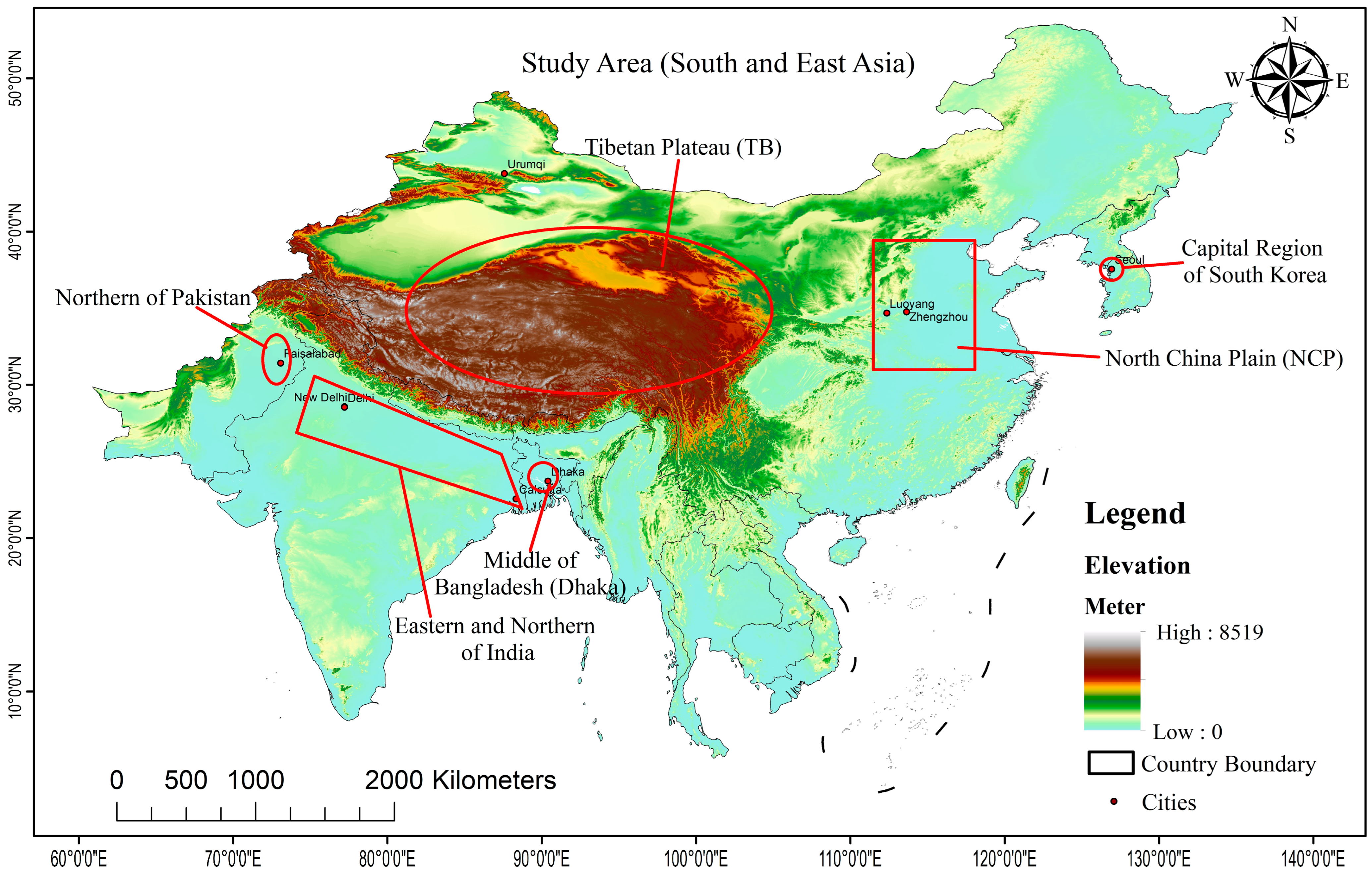
We leveraged gaseous pollutant data from satellite observations and ground-based monitoring to investigate the spatial and temporal characteristics of air pollution over a large area of Asia. OMI is onboarding the Aura satellite of NASA (National Aeronautics and Space Administration) for measuring trace gases with spatial resolution of 13 km × 24 km since 2004. This instrument provided estimates of atmospheric gaseous pollutants (NO2, SO2, O3, CO and other trace gases) in terms of back-scattered sunlight (passive remote sensing) from the Earth at ultraviolet and visible wavelengths [19].
The spectral range of Aura-OMI is 310.8 to 314.4 nm for SO2, and is 405 to 465 nm for NO2. The level 3 daily 0.25° × 0.25° tropospheric column NO2 product is used in this study for the period of 2011 to 2021 to focus on the last decade dynamics in air pollution over the study area. To ensure data quality, the data is used with cloud fraction of less than 0.3 and solar zenith angles of greater than 85º [42]. Similarly, the level 3 daily 0.25° × 0.25° total column SO2 in the PBL (Planetary boundary layer) is utilized here during 2011 to 2021. The best pixel is extracted by ensuring data quality with cloud fraction (<0.2), solar zenith angle (<20°) and row anomaly flags [43]. The cloud fraction of OMI data is acceptable on the column retrieval of trace gases (NO2, SO2, O3 etc.) because the Lambertian Cloud model is used with cloud albedo of 0.8, and the mass factor (the mean photon path) in the atmosphere at absorption line wavelength of a partly cloudy pixel is the weighted sum of the mass factor of the clear and cloudy part of the pixel [44,45,46,47].The Dutch-OMI-NO2 (DOMINO v2.0) algorithm and PCA (Principle Component Analysis) algorithm are used to estimate NO2, and SO2, respectively [48,49].
The AOD data is taken from the MODIS Aqua and Terra in ascending node at 550 nm with spatial resolution of 500 m. This product combines the dark target (DT) AOD for land and the deep blue (DB) AOD for ocean with normalized vegetation index (NDVI) statistics of greater than 0.3 for DT and less than 0.2 for DB [50]. The product is widely validated over global and/or regional area [51,52]. The combined MODIS AOD products with dark target (DT) over land utilized an excellent cloud rejection algorithm and maintaining high statistics of cloud free pixels [50]. In case of temporal differences, the OMI onboard Aura and the MODIS onboard Aqua are in very close time of local equator crossing with only 15 minutes’ difference in ascending node. Moreover, the utilized MODIS level 3 data was obtained from the MODIS level 2 AOD SWAT data with the quality flag of at least 2 (2 = good and 3 = very good).
In addition, the 0.1° × 0.1° monthly emission data from PKU emission inventory (2011–2014) is also used in this study to observe the overall spatial and temporal distribution of emissions over South and East Asia [53]. The summary of all utilized data is listed in Table S1 (see the Supplementary Material).

2.2 Study Region

This study evaluates spatiotemporal dynamics of air pollutants over South and East Asia, which lies between 60° E to 154° E and 5° N to 54° N as shown in Figure 1. Specifically, this study focuses on some highly polluted regions due to the rapid urbanization and industrialization [54] over China, Bangladesh, Pakistan, India, and Republic of Korea in the past decade. These countries including China, Bangladesh, India, Pakistan, and Republic of Korea are selected because the recent decades’ (last two decades) scenarios like urbanization, industrialization, population densities etc. are highly developing in the regions, which significantly increase the anthropogenic emissions (energy production, transportation, industry, residential and commercial, etc.). Here, the Tibetan Plateau is also selected because it is a special land of high altitude in this study area. The typical climate of South Asia is categorized as dry, temperate and tropical, while the typical climate of East Asia can be classified into five major zones: humid subtropical, humid continental, semiarid, arid, and highland [55]. Both study regions’ climate are highly influenced by monsoons [56,57].

2.3 Temporal Evaluation of Air Pollutants

The satellite-estimated data of NO2, SO2, and AOD are analyzed through a seasonal trend decomposition method to decompose the time series data into different components as [58]:
X(𝑡) = 𝑇(𝑡) × 𝑆(𝑡) × 𝐼(t),
where T(𝑡) is the trend component, S(𝑡) is the seasonal component, and I(𝑡) is the irregular component. Here, the statistical trend analysis is performed on the original monthly time-series and the 6-month moving average (MA) time-series to determine the average change in data over time (2011–2021). Additionally, the Mann-Kendall test is utilized to examine the trend of pollutants at pixel scale.
Along with the temporal evaluation of air pollutants, this study investigated the proportion of the mean pollutant column burden within each specific region relative to the mean air pollutant column burden across the entire study area. This analysis aims to elucidate the individual contribution of distinct areas or regions to the overall air pollution levels in East and South Asia. The proportion for NO2, SO2, or AOD over a specific area can be calculated as:
P N O 2 , S O 2 ,   o r   A O D = X s Y s
where P N O 2 , S O 2 ,   o r   A O D is the proportion of NO2, SO2, and AOD over a specific area relative to the whole study area, X s is the sum of annual area averaged air pollutants over a specific area like China, Bangladesh, Pakistan, India, etc., and Y s is the sum of annual area averaged air pollutants over the whole study area.

2.4 Hotspot Identification (Spatial Evaluation)

While a statistical measurement of higher or lower values of pollutant column density hold significance, its integration with geographical representation becomes even more crucial for a comprehensive spatial pattern analysis. The spatial clustering of higher or lower values is of utmost importance, and this can be effectively assessed using geospatial statistical tools, such as the Getis-Ord Gi* statistic as [59,60]:
G i * = j = 1 n w i , j ( x j x ¯ ) s n j = 1 n w i , j 2 j = 1 n w i , j 2 n 1 1 / 2
where x ¯ = j = 1 n x j n and s = j = 1 n x j 2 x ¯ 2 , x j is the prenominal value for a point j, w i , j = 1 r i , j is the measured distance of the j th point from the measurement point i, and n is the number of measuring points. This tool is applied by using the spatial statistical tools of ArcGIS 10.8 [61] to identify the hotspots of air pollutants.

3. Results

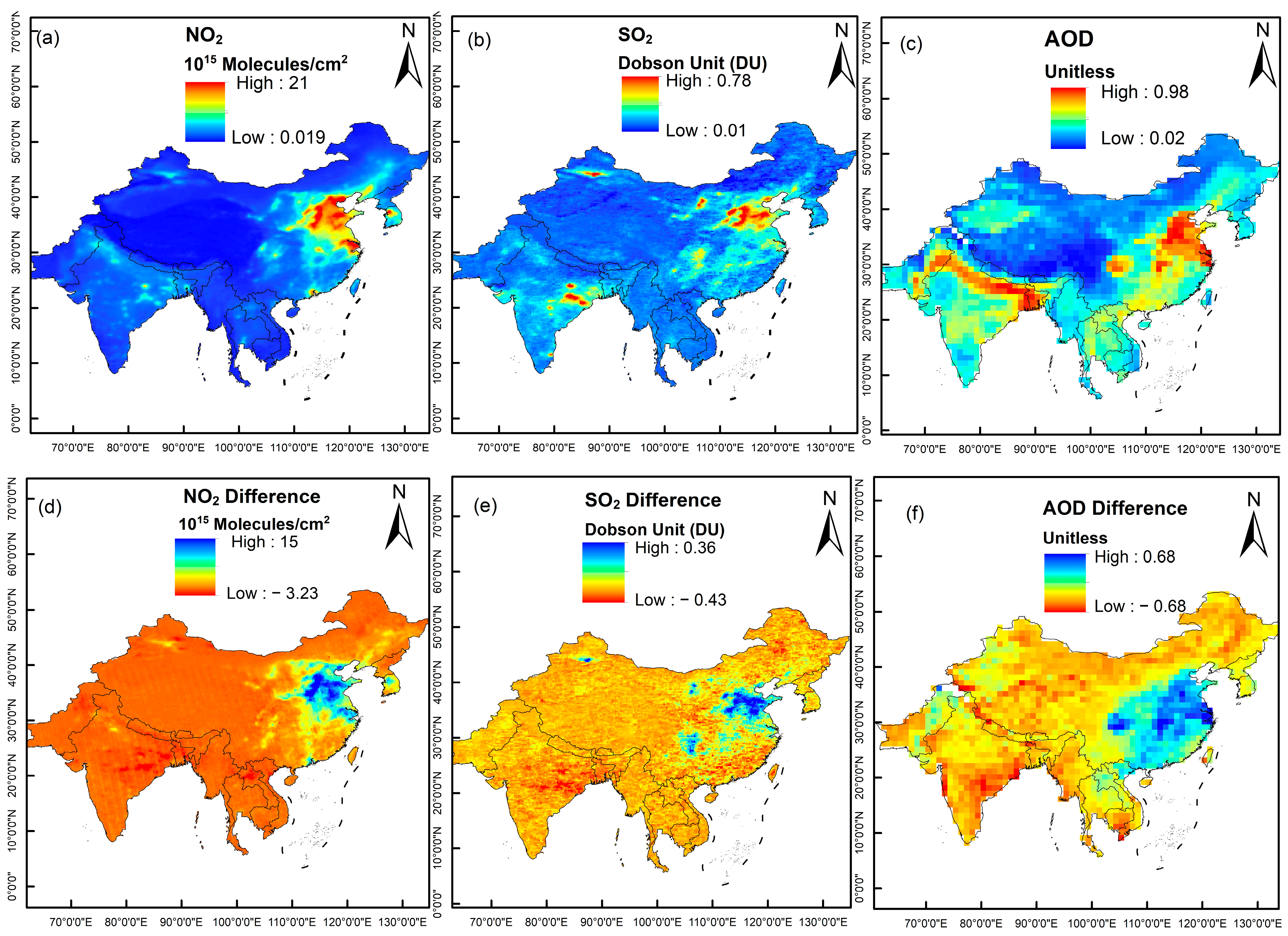
3.1 Spatial Distribution of NO2, SO2, and AOD

Figure 2a–c present the spatial distribution of the multi-year averaged (2011–2021) NO2, SO2, and AOD over South and East Asia during the period from 2011 to 2021, where the North China Plain (NCP) is characterized with higher values of NO2, SO2, and AOD, and some parts of Bangladesh, India, Pakistan, and S. Korea also have higher values of these air polluting components. Figure 2d–f shows the relative changes in NO2, SO2, and AOD between 2011 and 2021. The positive change indicated a reduction in emissions from 2011 to 2021, which is prominently observed over the NCP for all three air pollutants. Additionally, the eastern part of Republic of Korea has experienced a decline in NO2. In contrast, negative changes are observed for other study locations, signifying an increasing pattern of pollutant emissions.
We assessed seasonal variations in the spatial distribution of the relevant air pollutants, considering spring (March to May, MAM), summer (June to August, JJA), autumn (September to November, SON), and winter (December to February, DJF) as shown in Figures S1–S3 (see the Supplementary Material). The seasonal distribution of NO2 demonstrates low column densities in summer and high column densities in winter, and moderate values in other seasons. NCP exhibits a constantly higher NO2 level (~18.32 × 10¹⁵ molecules/cm2) throughout the year. The highest values are recorded in spring in the central (Capital, Dhaka, ~6.87 × 10¹⁵ molecules/cm2) and southern (Khulna, ~5.53 × 10¹⁵ molecules/cm2) regions of Bangladesh, eastern parts of India, and the capital region of Republic of Korea. SO2 also shows similar patterns in seasonal variations and spatial distributions over the study area. The AOD reflects opposite patterns compared to those of SO2 and NO2, with higher values in summer and spring and lower values in winter. Higher AOD in spring can be attributed to frequent dust events, and higher values in summer may be due to high humidity and photochemical transformation of SO2 and NO2 into sulfate and nitrate aerosols [35,62,63].

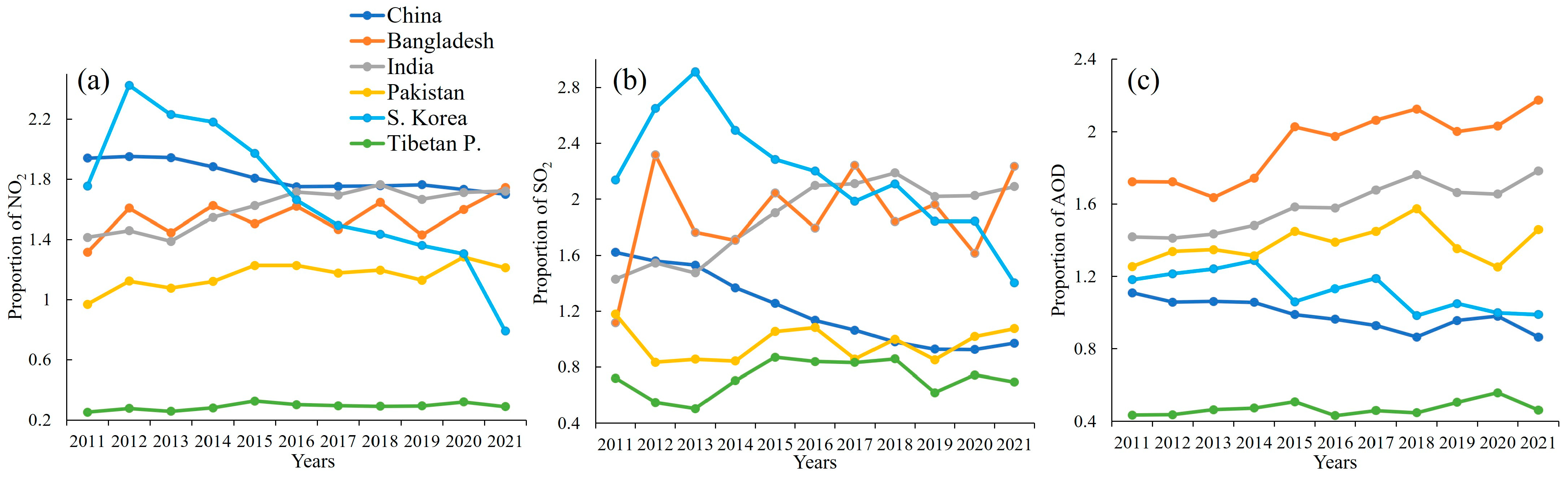
3.2 Regional Trend Analysis of NO2, SO2, and AOD

Figure 3 illustrates the pixel-wise trend distribution of NO2, SO2, and AOD from 2011 to 2021. Notably, the Mann-Kendall (MK) score for NO2 is negative and exhibits high values (depicted in green-colored regions on the map) predominantly over the North China Plain (NCP) and Republic of Korea. These findings signify pronounced decreasing trends in NO2 column densities within these regions. The positive MK score for NO2 with notably higher values over Bangladesh, India, and Pakistan, indicating strong increasing trends. Similar trends are also observed for SO2 and AOD (Figure 3a–c). The respective p-values of the trend analysis indicate statistically significance (<0.05) for the regions exhibiting strong increasing or decreasing trends (See Figure S4 in the Supplementary Material).
The area-averaged monthly changes in SO2 from 2011 to 2021 using the original monthly mean time-series and the 6-month moving average time-series over different regions are presented in Figure 4. The SO2 results indicate the decreasing (negative) trend over China and Republic of Korea with slopes of − 0 .0079 × 1015 molecules/cm2/year (−0.0078 × 10¹⁵ for moving average) and −0.0188 × 10¹⁵ molecules/cm2/year (−0.0201 × 10¹⁵ for moving average), respectively. There are positive (increasing) trends with slopes of 0.0011 × 10¹⁵ molecules/cm2/year, 0.0011 × 10¹⁵ molecules/cm2/year, 0.0004×10¹⁵ molecules/cm2/year, and 0.0005 × 10¹⁴ molecules/cm2/year over Bangladesh, India, Pakistan, and the Tibetan plateau, respectively. The overall trend analysis of NO2 and AOD also shows similar trends (see Figures S5 and S6 in the Supplementary Material). These monthly mean time series and their moving averages exhibit noticeable seasonal cycles of SO2 and NO2 with higher values in winter and lower values in summer, whereas AOD shows an opposite variation (i.e., lower in winter but higher in summer and spring). We also note that the magnitudes of NO2, SO2, and AOD are relatively lower in the year 2020, which is due to the weaker emissions during the lockdown period of the Covid-19 situation during 2020 [64,65].
Figure 5 presents the proportion of the three air pollutants for a specific region like China, Bangladesh, Pakistan, India, Republic of Korea and Tibetan Plateau which is calculated as the ratio of the sum of an air pollutant over a specific region to the sum of that air pollutant over the total study area. The area averaged data were extracted for each specific regions using the masking process of ArcGIS software, then converted in CSV format for each specific regions and for the whole study region, and finally performed the ratio operation. The proportion reflects the influences of an air pollutant in a specific region on the entire East and South Asia [41]. The proportion-analysis results of NO2 indicate that all regions have an influence (the proportion is >0.5) on the total NO2 except for the Tibetan Plateau. Two countries (China and Republic of Korea) show decreasing trends, and other countries (e.g., India, Bangladesh, and Pakistan) show increasing trends as discussed above. A similar trend from proportion analysis is found in the case of SO2 and AOD (Figure 5b,c) with the exception that the Tibetan Plateau also shows a slight influence on the total air pollution of SO2 and AOD. In addition, the proportion analysis for different regions (Figure 5) indicates a similar trend and all countries are influenced by air pollution (the proportion > 0.5), except for the Tibetan plateau, which is very slightly influenced by SO2 and AOD [41,66].

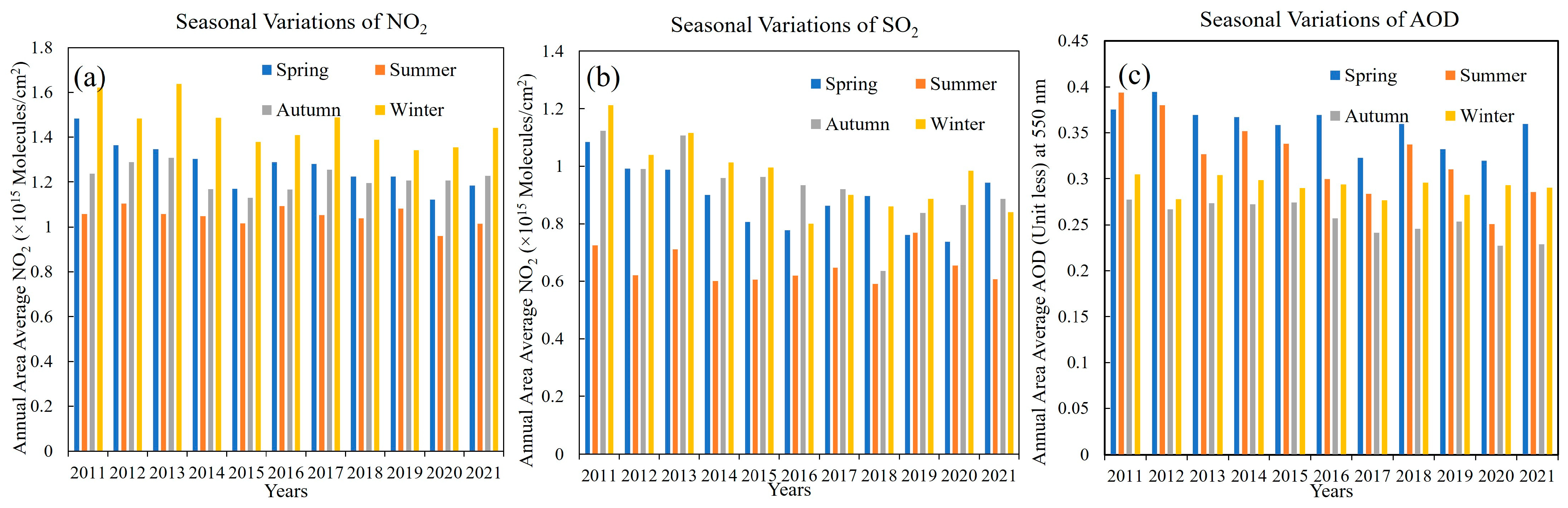
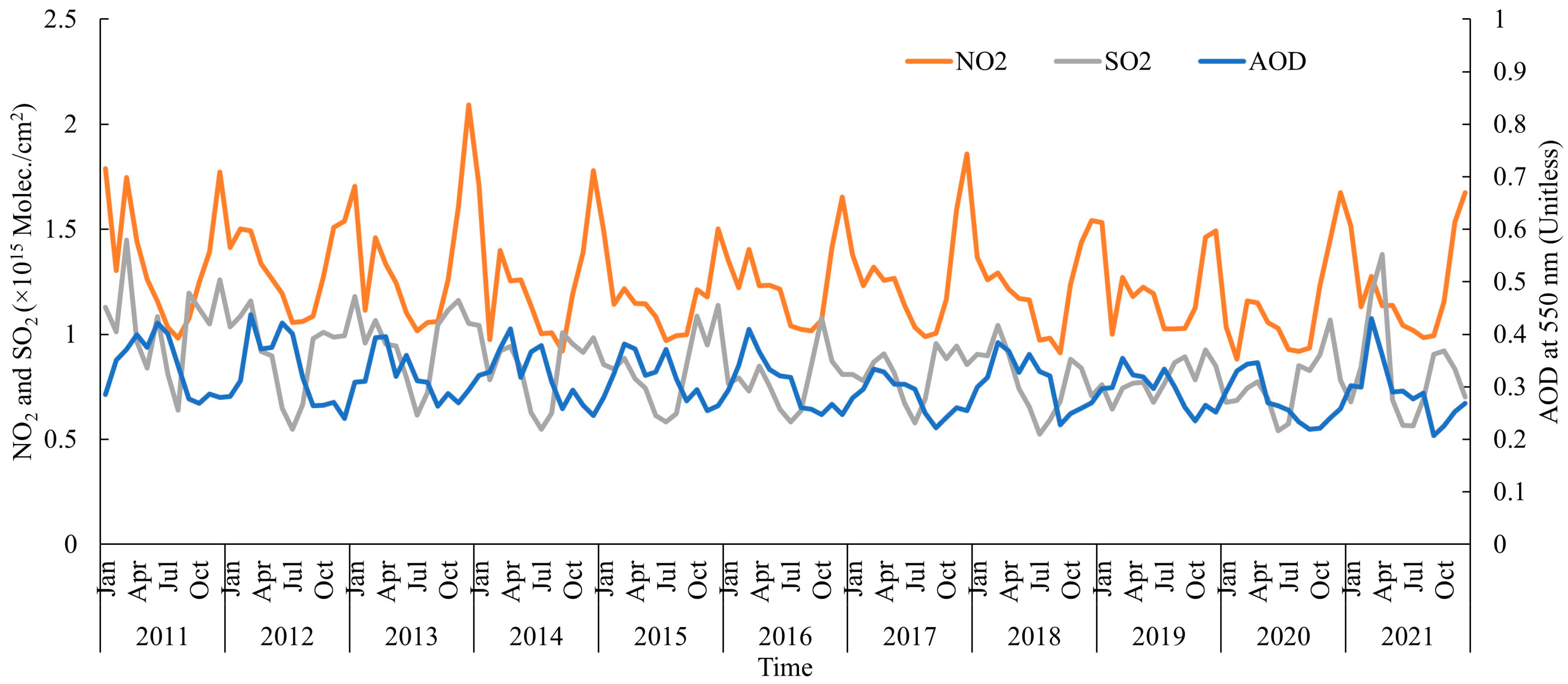
3.3 Seasonal Trend of Overall NO2, SO2, and AOD

Figure 6 illustrated the seasonal variations in NO2, SO2, and AOD from 2011 to 2021. Notably, the NO2 and SO2 are lowest in summer, which can be explained by wet deposition due to frequent precipitation and photochemical transformation of NO2 and SO2 into aerosols [17,67,68]. Higher values of NO2 and SO2 in winter and autumn may be due to the higher emissions from several burnings like house heating, brick kiln burnings, and agricultural crop residue burnings in East and South Asian regions [69,70]. The seasonal variations of AOD over the study area show an opposite behavior, with lower values found in winter and autumn but higher values found in spring and summer as shown in Figure 6c, which can be described by frequent dust events, higher humidity, and efficient photochemical conversion of NO2 and SO2 into sulfate and nitrate aerosols [62,63]. The comparison of the monthly (area averaged for the whole study area) time-series (2011–2021) shows that the AOD is also exhibiting the opposite relationship with NO2 and SO2 as shown in Figure 7.

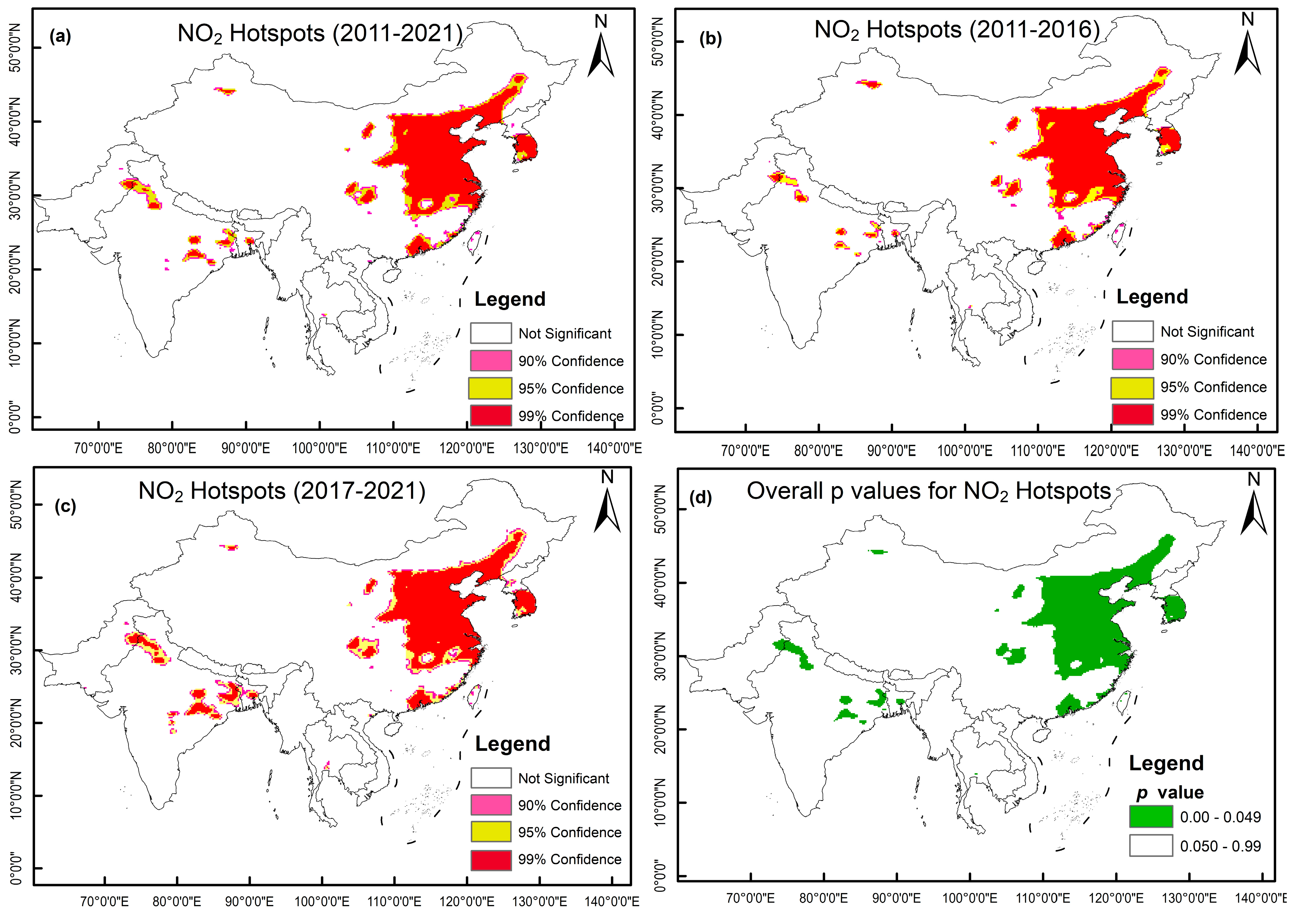
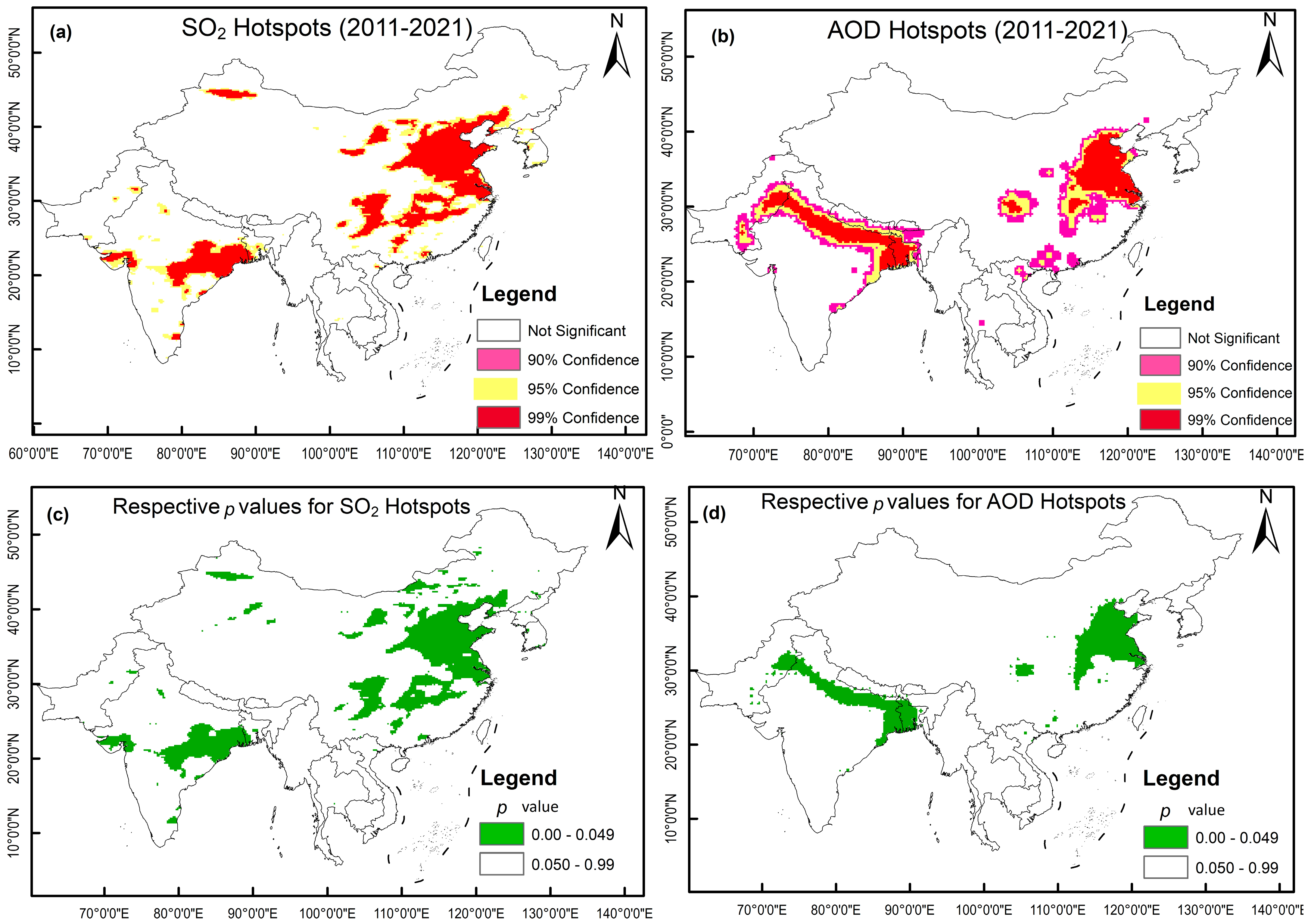
3.4 Hotspots Identification

The hotspot analysis is visualized using three different periods: first half (2011–2016), second half (2017–2021), and the entire time span (2011–2021) (Figure 8a–c, respectively) to confirm the realistic hotspots for NO2 with statistical significance. The three different periods’ hotspots show statistically significant results, where the hotspot areas are increasing in the second half (2017–2021) of the period as compared to the first half (2011–2016) over India, Bangladesh, and Pakistan. The statistical values of NO2 hotspots over randomly selected cities are shown in Table S2 (see Supplementary Material). Specifically, the economically developed cities over the study area are identified as statistically significant (>95% confidence and p-value <0.049) hotspots such as the NCP, the Yangtze River Delta (YRD), and the Pearl River Delta (PRD) in China, Republic of Korea, the central Bangladesh (Dhaka), some eastern (Calcutta) and northern parts (New Delhi, Amritsar) of India. Most of the identified hotspots are with the 95% to 99% confidence level. Figure 7d shows the respective p values which are also statistically significant for all the identified hotspots in the study area. Our results are aligned with the previous study [71].
This study also explores statistically significant hotspots of SO2 and AOD as shown in Figure 9. The hotspots of SO2 were mainly observed in the NCP, the eastern part of India as prolonged to the western part of Bangladesh, the capital area of Republic of Korea, and the industrialized areas of north-eastern Pakistan. While the AOD hotspots are mainly distributed over the whole of Bangladesh, northern India, the eastern part of Pakistan, and the NCP (Figure 9b). Based on the p values, the hotspots areas were statistically significant (<0.05) for SO2 and AOD, respectively (Figure 9c,d).

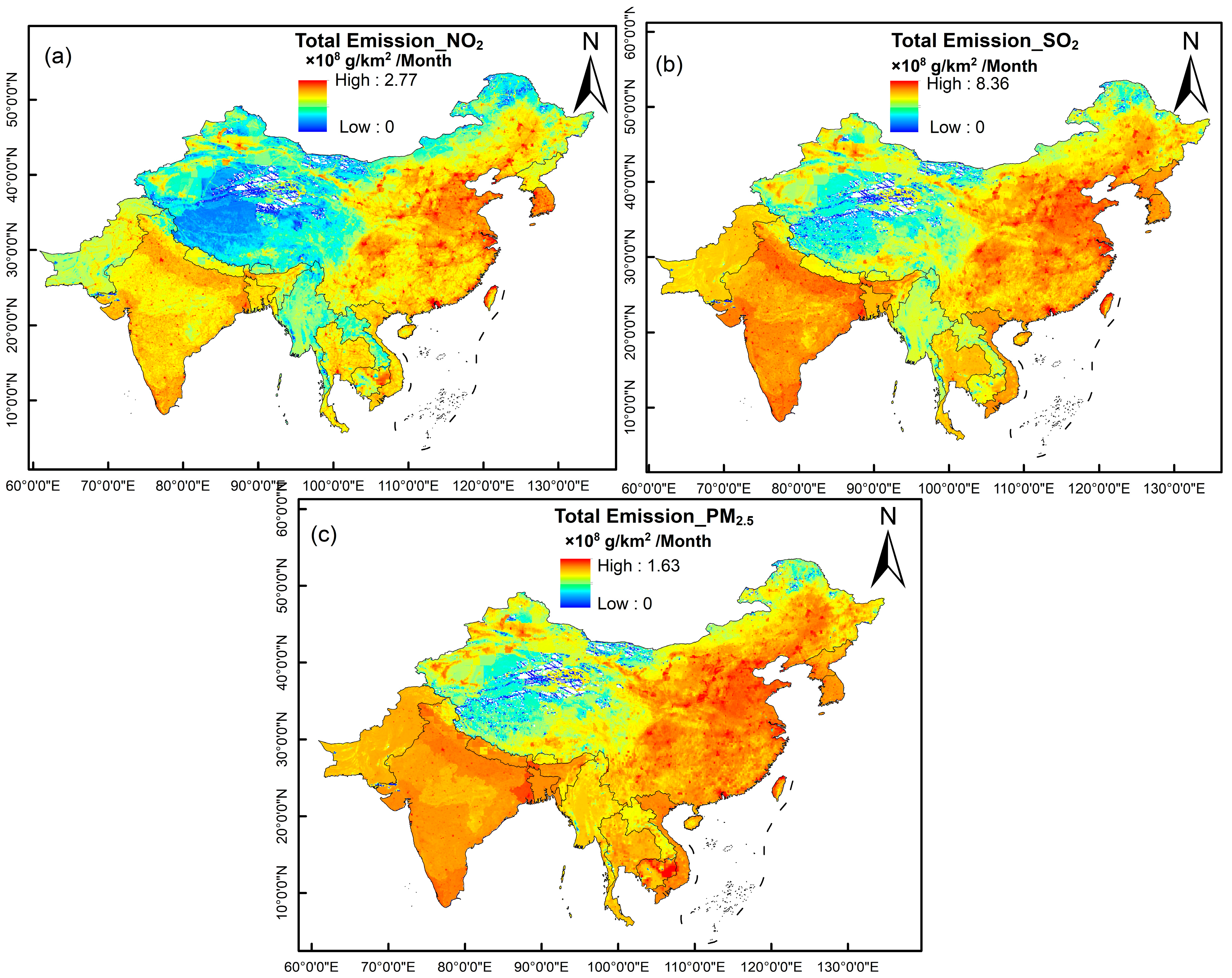
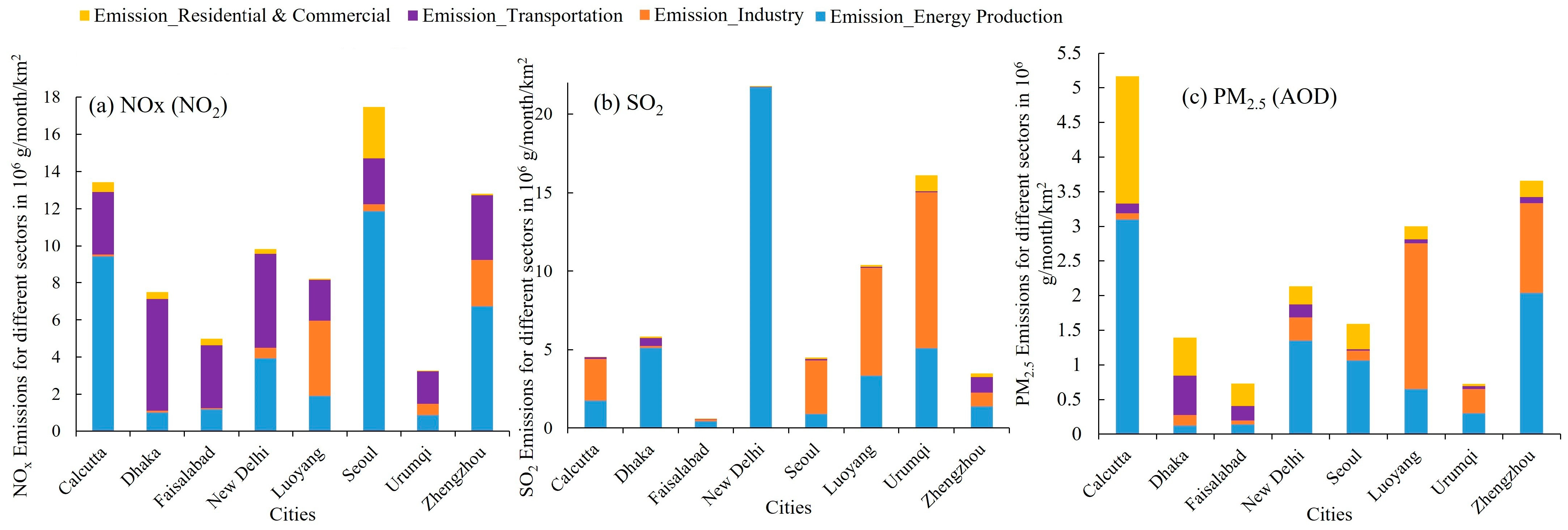
3.5 Emission Analysis of NOx, SO2, and PM2.5

The natural variation in air pollutants over the study area is negligible. For example, Kang et al. [4] analyzed the natural contribution to a multi-year (2007–2011) variation of NO2, SO2, and AOD over East Asia, and found that NO2 was increased by 76% with only 1% contributed by natural contribution and 99% contributed by anthropogenic contribution; SO2 was decreased by 15% with 16% contributed by natural contribution and 84% contributed by anthropogenic contribution; and AOD was increased by 24% with 23% contributed by natural contribution and 77% contributed by anthropogenic contribution. As a result, the anthropogenic contribution (the energy production, vehicle transportation, other fossil fuel burnings, household burnings etc.) is dominant (>85% on average) for these three pollutants in the study regions. This subsection focuses on examining the spatial distribution of emissions for the years 2011–2014. Additionally, it entails the analysis of sector-wise emission sources within the identified hotspots across the study area. The NOx (NO and NO2) emission inventory can be used for NO2 because NO is the primary pollutant which is further oxidized into NO2 [53,72]. As there is a good correlation between AOD (at 550 nm) and PM2.5 at the planetary boundary layer [73,74], the emission inventory of PM2.5 can also be used for AOD. The spatial distributions of total emissions (sum of emissions from all sectors) of NOx, SO2, and PM2.5, respectively, over East and South Asia were retrieved from the latest PKU (Peking University) emission inventory (http://inventory.pku.edu.cn/, accessed on 25 July 2022) [53,63,75]. The maximum values of NOx, SO2, and PM2.5 emissions are mainly over the NCP, northern and southern parts of India, northern Pakistan, and northern Republic of Korea, and the central part of Bangladesh as 2.77 × 10⁸ g/km2/month, 8.36 × 10⁸ g/km2/month, and 1.63 × 10⁸ g/km2/month, respectively (Figure 10a–c).
Figure 11 presents sector-wise emissions for the three air pollutants across eight economically developed and developing cities. The analysis primarily centers on emissions from energy production, industry, transportation, as well as residential and commercial sectors. NO2 emissions in various cities are significantly influenced by different sectors. Specifically, emissions from the energy production sector exhibit higher levels in cities such as Zhengzhou (China), Calcutta (India), and Seoul (Republic of Korea). On the other hand, emissions from the transportation sector dominate in cities like Dhaka (Bangladesh), Faisalabad (Pakistan), New Delhi (India), and Urumqi (China) (Figure 11a). In terms of SO2 emissions, the energy production sector contributes significantly to high emissions in cities such as New Delhi (India) and Dhaka (Bangladesh). Conversely, emissions of SO2 from the industrial sector are notably elevated in cities like Seoul (Republic of Korea), Urumqi (China), and Luoyang (China) (Figure 11b). The PM2.5 emissions from the energy production sector are higher mainly in Calcutta and New Delhi (India) as well as Seoul (Republic of Korea), while notably higher contributions from the industrial sector occur in cities like Luoyang (China) and Urumqi (China). Additionally, significant PM2.5 emissions are attributed to the residential and commercial sectors in Calcutta and Faisalabad, while the transportation sector dominates PM2.5 emissions in Dhaka. The results indicate that air pollution over different cities is highly/dominatingly impacted by different sectors’ emissions. The NO2 pollution over Dhaka, Faisalabad, and New Delhi is dominated by emissions from transportation, but it is dominated by emissions from the energy production sector in Zhengzhou, Seoul, and Calcutta. Thus, sector-wise emission analysis is necessary for making effective air pollution control policies over the study area.

4. Discussion

This study presents a comprehensive evaluation of the spatial and temporal trends of NO2, SO2, and AOD over East and South Asia using satellite-derived data from 2011 to 2021. The results highlight that there are declining trends of air pollution over China and Republic of Korea due to the well-planned and strict implementation of long-term air pollution control policies to reduce emissions [33,76]. Clear increasing trends of the concerned air pollutants are observed over Bangladesh, Pakistan, and India, which reflects that there is still lack of air pollution control policies and strict implementation in these regions. In fact, there are potential emissions from anthropogenic sources (industry, power plants, vehicle transportation, residential, commercial and all other biomass burning) and natural sources over these regions [77]. Now, it is the question of how Asia can reduce its emissions to a health-friendly level. As revealed by this study and other previous studies, some countries like China, Republic of Korea, and Japan are trying to incorporate huge amounts of renewable energy (wind, solar, and water-based energy) into the national power grid and to implement other air pollution control policies.
As per the existing literature on air pollution control policies, the most effective air pollution control policies were implemented by China [78,79,80,81], where they had to take several plans, actions and strict implementation during the process of air pollution control war. The following potential strategies can be recommended for countries (e.g., Bangladesh, Pakistan, and India) that are suffering from increasing trends in air pollution. One could establish the environmental governance to build the environmental regulatory system by using several administrative units like the Ministry of Environment, central and local environmental protection bureaus, and other structural institutions [81]. One could develop environmental laws and standards to notify the people at different legislative levels regarding the detailed standards as measured and recommended by different national and international organizations (e.g. EPA, WHO, NAAQS etc.) [82]. One could implement plans like the Five Year Plans (FYPs) on a local and national scale to achieve the target emissions reduction. For example, the FYP (2013–2017) in Beijing and its surroundings got a reduction of emissions by 83% for SO2, 43% for NOx, 42% for VOCs, and 59% for primary PM2.5 [78]. One could also select the target precursors (SO2, NOx, PM2.5, etc.) and sectors (energy production, industry, vehicle transportation, residential, agricultural etc.) based on the sector wise emission analysis [83]. One could take special actions in addition to the FYPs to control the special cases (special needs, crisis, and environmental accidents). For example the preparation of 2008 Olympic games in Beijing was needed for the special actions regardless of general regulations [84]. It is also necessary to identify the fundamental flaws in environmental regulations such as the absence of general principles of environmental rights and too low pollution punishment fee [80].
Therefore, the detailed trend analysis, hotspots analysis, and emission analysis in this study can help the policymakers to set air pollution control policies constructively in terms of the aforementioned points.

5. Conclusions

Overall, this study evaluated the spatial and temporal characteristics of NO2, SO2, and AOD over East and South Asia using satellite-derived data from 2011 to 2021. The trend analysis of these air pollution parameters indicated that two countries (China and Republic of Korea) have a declining rate in air pollution levels and emissions due to their well-planned emission reduction policies. However, based on the proportion analysis, we found that the contributions of air pollution in those countries to the total air pollution in the entire East and South Asia are still significant. The South Asian regions, particularly Bangladesh, India, and Pakistan, show significant increasing trends in air pollution, emphasizing the immediate implementation of long-term air pollution control policies to restrict the emissions. The seasonal variations of NO2, SO2, and AOD reflects the impacts of local emissions and meteorological conditions, and there is a passive inter-relationship between them as the increment of NO2 and SO2 will increase the secondary aerosol formation due to photochemical conversion into nitrate and sulfate aerosols. The results of the emission analysis implied that it is necessary to incorporate the sector-wise emission analysis in evaluating the impact of air pollution in different cities. For example, Dhaka, Faisalabad, and Calcutta are highly polluted with vehicle transportation, residential and commercial sectors compared to other sectors. The time-series and proportion analyses over the Tibetan Plateau suggests the motivation for systematic future work on air pollution specifically for SO2 and AOD over this high terrain region. Finally, the results and discussions in this study can be utilized by the policymakers for setting up integrated and/or separate air pollution control policies over East and South Asian regions.

Supplementary Materials

The following supporting information can be downloaded at: https://www.mdpi.com/article/10.3390/rs15205069/s1, Figure S1: Seasonal distribution of NO2 (in molecules/cm2) during the period from 2011 to 2021; Figure S2: Seasonal distribution of SO2 (in molecules/cm2) during the period from 2011 to 2021; Figure S3: Seasonal distribution of AOD (in molecules/cm2) during the period from 2011 to 2021; Figure S4: Respective p-values for the regional distributions of the trends of (a) NO2, (b) SO2, and (c) AOD; Figure S5: The overall trend of NO2 over (a) China, (b) Bangladesh, (c) India, (d) Pakistan, (e) Republic of Korea, and (f) Tibetan Plateau; Figure S6: The overall trend of AOD over (a) China, (b) Bangladesh, (c) India, (d) Pakistan, (e) Republic of Korea, and (f) Tibetan Plateau.

Author Contributions

Conceptualization, M.M.R. and S.W.; methodology, M.M.R.; software, M.M.R. and A.A.; formal analysis, M.M.R.; investigation, M.M.R. and S.W.; data curation, M.M.R.; writing—original draft preparation, M.M.R.; writing—review and editing, M.M.R., S.W. and C.H.; visualization, M.M.R.; supervision, W.Z. (Weixiong Zhao); project administration, W.Z. (Weixiong Zhao) and W.Z. (Weijun Zhang). All authors have read and agreed to the published version of the manuscript.

Funding

This research was funded by the Chinese Academy of Sciences (CAS) President’s International Fellowship Initiative (PIFI) (Grant 2020PE0030), the National Natural Science Foundation of China (42022051), the Youth Innovation Promotion Association CAS (Y202089), the Natural Science Foundation of Anhui Province (2108085QD181), and HFIPS Director’s Fund (YZJJ2021QN02).

Data Availability Statement

No new data were created and/or data are unavailable due to privacy or ethical restrictions.

Acknowledgments

This study wishes to acknowledge the intellectual contribution of the Department of Electrical and Electronic Engineering, Pabna University of Science and Technology, Pabna-6600, Bangladesh. This study also wishes to acknowledge NASA’s Earth Data portal and Peking University’s (PKU) emissions inventory.

Conflicts of Interest

The authors declare no conflict of interest.

References

  1. Lu, Z.; Zhang, Q.; Streets, D.G. Sulfur Dioxide and Primary Carbonaceous Aerosol Emissions in China and India, 1996–2010. Atmos. Chem. Phys. 2011, 11, 9839–9864. [Google Scholar] [CrossRef]
  2. Mulholland, E.; Miller, J.; Bernard, Y.; Lee, K.; Rodríguez, F. The Role of NO x Emission Reductions in Euro 7/VII Vehicle Emission Standards to Reduce Adverse Health Impacts in the EU27 through 2050. Transp. Eng. 2022, 9, 100133. [Google Scholar] [CrossRef]
  3. Kampa, M.; Castanas, E. Human Health Effects of Air Pollution. Environ. Pollut. 2008, 151, 362–367. [Google Scholar] [CrossRef] [PubMed]
  4. Kang, H.; Zhu, B.; van der, A.R.J.; Zhu, C.; de Leeuw, G.; Hou, X.; Gao, J. Natural and Anthropogenic Contributions to Long-Term Variations of SO2, NO2, CO, and AOD over East China. Atmos. Res. 2019, 215, 284–293. [Google Scholar] [CrossRef]
  5. Acharya, P.; Barik, G.; Gayen, B.K.; Bar, S.; Maiti, A.; Sarkar, A.; Ghosh, S.; De, S.K.; Sreekesh, S. Revisiting the Levels of Aerosol Optical Depth in South-Southeast Asia, Europe and USA amid the COVID-19 Pandemic Using Satellite Observations. Environ. Res. 2021, 193, 110514. [Google Scholar] [CrossRef]
  6. Mohammadi, M.; Neshat, E. Accurate Prediction of NOx Emissions from Diesel Engines Considering In-Cylinder Ion Current. Environ. Pollut. 2020, 266, 115347. [Google Scholar] [CrossRef]
  7. Olivier, J.G.J.; Bouwman, A.F.; Van Der Hoek, K.W.; Berdowski, J.J.M. Global Air Emission Inventories for Anthropogenic Sources of NO(x), NH3 and N2O in 1990. Environ. Pollut. 1998, 102, 135–148. [Google Scholar] [CrossRef]
  8. Eckel, S.P.; Cockburn, M.; Shu, Y.H.; Deng, H.; Lurmann, F.W.; Liu, L.; Gilliland, F.D. Air Pollution Affects Lung Cancer Survival. Thorax 2016, 71, 891–898. [Google Scholar] [CrossRef]
  9. EPA Final Integrated Science Assessment for Oxides of Nitrogen, Oxides of Sulfur, and Particulate Matter—Current Review of the Air Quality Criteria for the Particulate Matter NAAQS. EPA. Fed. Regist. 2020, 85, 66327–66328.
  10. He, X.; Pang, S.; Ma, J.; Zhang, Y. Influence of Relative Humidity on Heterogeneous Reactions of O3 and O3/SO2 with Soot Particles: Potential for Environmental and Health Effects. Atmos. Environ. 2017, 165, 198–206. [Google Scholar] [CrossRef]
  11. Li, R.; Cui, L.; Meng, Y.; Zhao, Y.; Fu, H. Satellite-Based Prediction of Daily SO2 Exposure across China Using a High-Quality Random Forest-Spatiotemporal Kriging (RF-STK) Model for Health Risk Assessment. Atmos. Environ. 2019, 208, 10–19. [Google Scholar] [CrossRef]
  12. Rupakheti, D.; Rupakheti, M.; Rai, M.; Yu, X.; Yin, X.; sKang, S.; Orozaliev, M.D.; Sinyakov, V.P.; Abdullaev, S.F.; Sulaymon, I.D.; et al. Characterization of Columnar Aerosol over a Background Site in Central Asia. Environ. Pollut. 2023, 316, 120501. [Google Scholar] [CrossRef] [PubMed]
  13. Ramachandran, S.; Rupakheti, M. Trends in Physical, Optical and Chemical Columnar Aerosol Characteristics and Radiative Effects over South and East Asia: Satellite and Ground-Based Observations. Gondwana Res. 2022, 105, 366–387. [Google Scholar] [CrossRef]
  14. Khamraev, K.; Cheriyan, D.; Choi, J. A Review on Health Risk Assessment of PM in the Construction Industry—Current Situation and Future Directions. Sci. Total Environ. 2021, 758, 143716. [Google Scholar] [CrossRef]
  15. Pateraki, S.; Manousakas, M.; Bairachtari, K.; Kantarelou, V.; Eleftheriadis, K.; Vasilakos, C.; Assimakopoulos, V.D.; Maggos, T. The Traffic Signature on the Vertical PM Profile: Environmental and Health Risks within an Urban Roadside Environment. Sci. Total Environ. 2019, 646, 448–459. [Google Scholar] [CrossRef]
  16. Faria, T.; Martins, V.; Canha, N.; Diapouli, E.; Manousakas, M.; Fetfatzis, P.; Gini, M.I.; Almeida, S.M. Assessment of Children’s Exposure to Carbonaceous Matter and to PM Major and Trace Elements. Sci. Total Environ. 2022, 807, 151021. [Google Scholar] [CrossRef]
  17. Rahman, M.M.; Shuo, W.; Zhao, W.; Xu, X.; Zhang, W.; Arshad, A. Investigating the Relationship between Air Pollutants and Meteorological Parameters Using Satellite Data over Bangladesh. Remote Sens. 2022, 14, 2757. [Google Scholar] [CrossRef]
  18. NASA Aura | OMI. Images, Data, Inf. Atmos. Ozone 2020. Available online: https://aura.gsfc.nasa.gov/omi.html (accessed on 20 May 2022).
  19. Levelt, P.F.; Van Den Oord, G.H.J.; Dobber, M.R.; Mälkki, A.; Visser, H.; De Vries, J.; Stammes, P.; Lundell, J.O.V.; Saari, H. The Ozone Monitoring Instrument. IEEE Trans. Geosci. Remote Sens. 2006, 44, 1093–1100. [Google Scholar] [CrossRef]
  20. Meijer, Y.J.; Swart, D.P.J.; Baier, F.; Bhartia, P.K.; Bodeker, G.E.; Casadio, S.; Chance, K.; Del Frate, F.; Erbertseder, T.; Felder, M.D.; et al. Evaluation of Global Ozone Monitoring Experiment (GOME) Ozone Profiles from Nine Different Algorithms. J. Geophys. Res. Atmos. 2006, 111, 1–28. [Google Scholar] [CrossRef]
  21. Team of MOPITT, N. MOPITT Measurement of Pollution in the Troposphere. J. Atmos. Ocean. Technol. 1996, 13, 314–320. [Google Scholar]
  22. Buchwitz, M.; Khlystova, I.; Bovensmann, H.; Burrows, J.P. Three Years of Global Carbon Monoxide from SCIAMACHY: Comparison with MOPITT and First Results Related to the Detection of Enhanced CO over Cities. Atmos. Chem. Phys. 2007, 7, 2399–2411. [Google Scholar] [CrossRef]
  23. Choi, H.; Liu, X.; Jeong, U.; Chong, H.; Kim, J.; Ahn, M.H.; Ko, D.H.; Lee, D.; Moon, K.-J.; Lee, K.-M. Geostationary Environment Monitoring Spectrometer (GEMS) Polarization Characteristics and Correction Algorithm. Atmos. Meas. Tech. Discuss. 2023, 2023, 1–33. [Google Scholar]
  24. Krotkov, N.A.; McClure, B.; Dickerson, R.R.; Carn, S.A.; Li, C.; Bhartia, P.K.; Yang, K.; Krueger, A.J.; Li, Z.; Levelt, P.F.; et al. Validation of SO2 Retrievals from the Ozone Monitoring Instrument over NE China. J. Geophys. Res. Atmos. 2008, 113, 1–13. [Google Scholar] [CrossRef]
  25. Hilboll, A.; Richter, A.; Burrows, J.P. Long-Term Changes of Tropospheric NO2 over Megacities Derived from Multiple Satellite Instruments. Atmos. Chem. Phys. 2013, 13, 4145–4169. [Google Scholar] [CrossRef]
  26. Karbasi, S.; Malakooti, H.; Rahnama, M.; Azadi, M. Study of Mid-Latitude Retrieval XCO2 Greenhouse Gas: Validation of Satellite-Based Shortwave Infrared Spectroscopy with Ground-Based TCCON Observations. Sci. Total Environ. 2022, 836, 155513. [Google Scholar] [CrossRef]
  27. Russell, A.R.; Valin, L.C.; Cohen, R.C. Trends in OMI NO2 Observations over the United States: Effects of Emission Control Technology and the Economic Recession. Atmos. Chem. Phys. 2012, 12, 12197–12209. [Google Scholar] [CrossRef]
  28. Rahman, M.M.; Zhang, W. Validation of Satellite-Derived Sensible Heat Flux for TERRA/MODIS Images over Three Different Landscapes Using Large Aperture Scintillometer and Eddy Covariance Measurements. IEEE J. Sel. Top. Appl. Earth Obs. Remote Sens. 2019, 12, 3327–3337. [Google Scholar] [CrossRef]
  29. Anastasopolos, A.T.; Sofowote, U.M.; Hopke, P.K.; Rouleau, M.; Shin, T.; Dheri, A.; Peng, H.; Kulka, R.; Gibson, M.D.; Farah, P.M.; et al. Air Quality in Canadian Port Cities after Regulation of Low-Sulphur Marine Fuel in the North American Emissions Control Area. Sci. Total Environ. 2021, 791, 147949. [Google Scholar] [CrossRef]
  30. O’Leary, B.F.; Hill, A.B.; Akers, K.G.; Esparra-Escalera, H.J.; Lucas, A.; Raoufi, G.; Huang, Y.; Mariscal, N.; Mohanty, S.K.; Tummala, C.M.; et al. Air Quality Monitoring and Measurement in an Urban Airshed: Contextualizing Datasets from the Detroit Michigan Area from 1952 to 2020. Sci. Total Environ. 2022, 809, 152120. [Google Scholar] [CrossRef]
  31. Fioletov, V.; McLinden, C.A.; Kharol, S.K.; Krotkov, N.A.; Li, C.; Joiner, J.; Moran, M.D.; Vet, R.; Visschedijk, A.J.H.; Denier Van Der Gon, H.A.C. Multi-Source SO2 Emission Retrievals and Consistency of Satellite and Surface Measurements with Reported Emissions. Atmos. Chem. Phys. 2017, 17, 12597–12616. [Google Scholar] [CrossRef]
  32. Krotkov, N.A.; McLinden, C.A.; Li, C.; Lamsal, L.N.; Celarier, E.A.; Marchenko, S.V.; Swartz, W.H.; Bucsela, E.J.; Joiner, J.; Duncan, B.N.; et al. Aura OMI Observations of Regional SO2 and NO2 Pollution Changes from 2005 to 2015. Atmos. Chem. Phys. 2016, 16, 4605–4629. [Google Scholar] [CrossRef]
  33. Li, C.; Hammer, M.S.; Zheng, B.; Cohen, R.C. Accelerated Reduction of Air Pollutants in China, 2017–2020. Sci. Total Environ. 2022, 803, 150011. [Google Scholar] [CrossRef] [PubMed]
  34. Liu, X.; Guo, C.; Wu, Y.; Huang, C.; Lu, K.; Zhang, Y.; Duan, L.; Cheng, M.; Chai, F.; Mei, F.; et al. Evaluating Cost and Benefit of Air Pollution Control Policies in China: A Systematic Review. J. Environ. Sci. 2023, 123, 140–155. [Google Scholar] [CrossRef]
  35. Lin, C.A.; Chen, Y.C.; Liu, C.Y.; Chen, W.T.; Seinfeld, J.H.; Chou, C.C.K. Satellite-Derived Correlation of SO2, NO2, and Aerosol Optical Depth with Meteorological Conditions over East Asia from 2005 to 2015. Remote Sens. 2019, 11, 1738. [Google Scholar] [CrossRef]
  36. Wang, S.X.; Zhao, B.; Cai, S.Y.; Klimont, Z.; Nielsen, C.P.; Morikawa, T.; Woo, J.H.; Kim, Y.; Fu, X.; Xu, J.Y.; et al. Emission Trends and Mitigation Options for Air Pollutants in East Asia. Atmos. Chem. Phys. 2014, 14, 6571–6603. [Google Scholar] [CrossRef]
  37. Pozzer, A.; De Meij, A.; Yoon, J.; Tost, H.; Georgoulias, A.K.; Astitha, M. AOD Trends during 2001–2010 from Observations and Model Simulations. Atmos. Chem. Phys. 2015, 15, 5521–5535. [Google Scholar] [CrossRef]
  38. He, Q.; Gao, K.; Zhang, L.; Song, Y.; Zhang, M. Satellite-Derived 1-Km Estimates and Long-Term Trends of PM2.5 Concentrations in China from 2000 to 2018. Environ. Int. 2021, 156, 106726. [Google Scholar] [CrossRef]
  39. Si, Y.; Yu, C.; Zhang, L.; Zhu, W.; Cai, K.; Cheng, L.; Chen, L.; Li, S. Assessment of Satellite-Estimated near-Surface Sulfate and Nitrate Concentrations and Their Precursor Emissions over China from 2006 to 2014. Sci. Total Environ. 2019, 669, 362–376. [Google Scholar] [CrossRef]
  40. Li, Y.; Ma, Q.; Chen, J.; Li, R.; Liu, B.; Qian, M.; Wang, Z. Long Term Variation Analysis of Satellite-Derived Air Pollution Components over East China. Int. Geosci. Remote Sens. Symp. 2018, 2018, 9134–9137. [Google Scholar] [CrossRef]
  41. Xie, Y.; Wang, W.; Wang, Q. Spatial Distribution and Temporal Trend of Tropospheric NO2 over the Wanjiang City Belt of China. Adv. Meteorol. 2018, 2018, 6597186. [Google Scholar] [CrossRef]
  42. Lamsal, N.L.; Krotkov, A.N.; Vasilkov, A.; Marchenko, S.; Qin, W.; Fasnacht, Z.; Joiner, J.; Choi, S.; Haffner, D.; Swartz, H.W.; et al. Ozone Monitoring Instrument (OMI) Aura Nitrogen Dioxide Standard Product Version 4.0 with Improved Surface and Cloud Treatments. Atmos. Meas. Tech. 2021, 14, 455–479. [Google Scholar] [CrossRef]
  43. Li, C.; Krotkov, N.A.; Leonard, P.J.T.; Carn, S.; Joiner, J.; Spurr, R.J.D.; Vasilkov, A. Version 2 Ozone Monitoring Instrument SO2 Product (OMSO2 V2): New Anthropogenic SO2 Vertical Column Density Dataset. Atmos. Meas. Tech. 2020, 13, 6175–6191. [Google Scholar] [CrossRef]
  44. Boersma, K.F.; Eskes, H.J.; Brinksma, E.J. Error Analysis for Tropospheric NO2 Retrieval from Space. J. Geophys. Res. Atmos. 2004, 109, 1–20. [Google Scholar] [CrossRef]
  45. Veefkind, J.P.; Bhartia, P.K.; Gleason, J.; de Haan, J.F.; Wellemeyer, C.; Qin, W.; Levelt, P.F. Total Ozone from the Ozone Monitoring Instrument (OMI) Using TOMS and DOAS Methods; European Geophysical Society: Nice, France, 2003; Volume 44, p. 8932. [Google Scholar]
  46. Joiner, J.; Vasilkov, A.P. First Results from the OMI Rotational Raman Scattering Cloud Pressure Algorithm. IEEE Trans. Geosci. Remote Sens. 2006, 44, 1272–1281. [Google Scholar] [CrossRef]
  47. Stammes, P.; Sneep, M.; de Haan, J.F.; Veefkind, J.P.; Wang, P.; Levelt, P.F. Effective Cloud Fractions from the Ozone Monitoring Instrument: Theoretical Framework and Validation. J. Geophys. Res. Atmos. 2008, 113, 1–12. [Google Scholar] [CrossRef]
  48. Li, C.; Joiner, J.; Krotkov, N.A.; Bhartia, P.K. A Fast and Sensitive New Satellite SO2 Retrieval Algorithm Based on Principal Component Analysis: Application to the Ozone Monitoring Instrument. Geophys. Res. Lett. 2013, 40, 6314–6318. [Google Scholar] [CrossRef]
  49. Boersma, K.F.; Eskes, H.J.; Dirksen, R.J.; Van Der, A.R.J.; Veefkind, J.P.; Stammes, P.; Huijnen, V.; Kleipool, Q.L.; Sneep, M.; Claas, J.; et al. An Improved Tropospheric NO2 Column Retrieval Algorithm for the Ozone Monitoring Instrument. Atmos. Meas. Tech. 2011, 4, 1905–1928. [Google Scholar] [CrossRef]
  50. Levy, R.C.; Mattoo, S.; Munchak, L.A.; Remer, L.A.; Sayer, A.M.; Patadia, F.; Hsu, N.C. The Collection 6 MODIS Aerosol Products over Land and Ocean. Atmos. Meas. Tech. 2013, 6, 2989–3034. [Google Scholar] [CrossRef]
  51. Zhu, J.; Xia, X.; Che, H.; Wang, J.; Cong, Z.; Zhao, T.; Kang, S.; Zhang, X.; Yu, X.; Zhang, Y. Spatiotemporal Variation of Aerosol and Potential Long-Range Transport Impact over the Tibetan Plateau, China. Atmos. Chem. Phys. 2019, 19, 14637–14656. [Google Scholar] [CrossRef]
  52. Bilal, M.; Nazeer, M.; Qiu, Z.; Ding, X.; Wei, J. Global Validation of MODIS C6 and C6.1 Merged Aerosol Products over Diverse Vegetated Surfaces. Remote Sens. 2018, 10, 6–9. [Google Scholar] [CrossRef]
  53. Huang, T.; Zhu, X.; Zhong, Q.; Yun, X.; Meng, W.; Li, B.; Ma, J.; Zeng, E.Y.; Tao, S. Spatial and Temporal Trends in Global Emissions of Nitrogen Oxides from 1960 to 2014. Environ. Sci. Technol. 2017, 51, 7992–8000. [Google Scholar] [CrossRef] [PubMed]
  54. Li, H.; Zhang, Q.; Zhang, Q.; Chen, C.; Wang, L.; Wei, Z.; Zhou, S.; Parworth, C.; Zheng, B.; Canonaco, F.; et al. Wintertime Aerosol Chemistry and Haze Evolution in an Extremely Polluted City of the North China Plain: Significant Contribution from Coal and Biomass Combustion. Atmos. Chem. Phys. 2017, 17, 4751–4768. [Google Scholar] [CrossRef]
  55. UNESCO Climate Fact Sheet-Asia Pacific; UNESCO: Paris, France, 2021; Volume 2.
  56. Ren, G.; Chan, J.C.L.; Kubota, H.; Zhang, Z.; Li, J.; Zhang, Y.; Zhang, Y.; Yang, Y.; Ren, Y.; Sun, X.; et al. Historical and Recent Change in Extreme Climate over East Asia. Clim. Change 2021, 168, 22. [Google Scholar] [CrossRef] [PubMed]
  57. Naveendrakumar, G.; Vithanage, M.; Kwon, H.H.; Chandrasekara, S.S.K.; Iqbal, M.C.M.; Pathmarajah, S.; Fernando, W.C.D.K.; Obeysekera, J. South Asian Perspective on Temperature and Rainfall Extremes: A Review. Atmos. Res. 2019, 225, 110–120. [Google Scholar] [CrossRef]
  58. Cleveland, R.B.; Cleveland, W.S.; McRae, J.E.T. STL: A Seasonal-Trend Decomposition Procedure Based on Loess. Nucl. Struct. Study Neutrons 1990, 6, 3–73. [Google Scholar] [CrossRef]
  59. Getis, A.; Ord, J.K. The Analysis of Spatial Association by Use of Distance Statistics. Geogr. Anal. 1992, 24, 189–206. [Google Scholar] [CrossRef]
  60. Ord, J.K.; Getis, A. Local Spatial Autocorrelation Statistics: Distributional Issues and an Application. Geogr. Anal. 1995, 27, 286–306. [Google Scholar] [CrossRef]
  61. ESRI ArcGIS Pro Resources | Tutorials, Documentation, Videos & More. ArcGIS Resour. 2015. Available online: https://www.esri.com/en-us/arcgis/products/arcgis-pro/resources (accessed on 15 January 2023).
  62. Khoder, M.I. Atmospheric Conversion of Sulfur Dioxide to Particulate Sulfate and Nitrogen Dioxide to Particulate Nitrate and Gaseous Nitric Acid in an Urban Area. Chemosphere 2002, 49, 675–684. [Google Scholar] [CrossRef]
  63. Wang, S.; Zhao, W.; Xu, X.; Fang, B.; Zhang, Q.; Qian, X.; Zhang, W.; Chen, W.; Pu, W.; Wang, X. Dependence of Columnar Aerosol Size Distribution, Optical Properties, and Chemical Components on Regional Transport in Beijing. Atmos. Environ. 2017, 169, 128–139. [Google Scholar] [CrossRef]
  64. Rojas, N.Y.; Ramírez, O.; Belalcázar, L.C.; Méndez-Espinosa, J.F.; Vargas, J.M.; Pachón, J.E. PM2.5 Emissions, Concentrations and Air Quality Index during the COVID-19 Lockdown. Environ. Pollut. 2021, 272, 2020–2021. [Google Scholar] [CrossRef]
  65. Wang, Y.; Wu, R.; Liu, L.; Yuan, Y.; Liu, C.G.; Hang Ho, S.S.; Ren, H.; Wang, Q.; Lv, Y.; Yan, M.; et al. Differential Health and Economic Impacts from the COVID-19 Lockdown between the Developed and Developing Countries: Perspective on Air Pollution. Environ. Pollut. 2022, 293, 118544. [Google Scholar] [CrossRef]
  66. Wang, C.; Wang, T.; Wang, P. The Spatial-Temporal Variation of Tropospheric NO2 over China during 2005 to 2018. Atmosphere 2019, 10, 444. [Google Scholar] [CrossRef]
  67. Zannetti, P. Dry and Wet Deposition. In Air Pollution Modeling; Springer: Boston, MA, USA, 1990; pp. 249–262. [Google Scholar] [CrossRef]
  68. Wałaszek, K.; Kryza, M.; Dore, A.J. The Impact of Precipitation on Wet Deposition of Sulphur and Nitrogen Compounds. Ecol. Chem. Eng. S 2013, 20, 733–745. [Google Scholar] [CrossRef]
  69. Yin, S. Biomass Burning Spatiotemporal Variations over South and Southeast Asia. Environ. Int. 2020, 145, 106153. [Google Scholar] [CrossRef]
  70. Korontzi, S.; McCarty, J.; Loboda, T.; Kumar, S.; Justice, C. Global Distribution of Agricultural Fires in Croplands from 3 Years of Moderate Resolution Imaging Spectroradiometer (MODIS) Data. Global Biogeochem. Cycles 2006, 20, 1–15. [Google Scholar] [CrossRef]
  71. Ul-Haq, Z.; Tariq, S.; Ali, M. Tropospheric NO2 Trends over South Asia during the Last Decade (2004–2014) Using OMI Data. Adv. Meteorol. 2015, 2015, 959284. [Google Scholar] [CrossRef]
  72. Jamali, S.; Klingmyr, D.; Tagesson, T. Global-Scale Patterns and Trends in Tropospheric NO2 Concentrations, 2005–2018. Remote Sens. 2020, 12, 3526. [Google Scholar] [CrossRef]
  73. Kumar, N.; Chu, A.; Foster, A. An Empirical Relationship between PM 2.5 and Aerosol Optical Depth in Delhi Metropolitan. Atmos. Environ. 2007, 41, 4492–4503. [Google Scholar] [CrossRef] [PubMed]
  74. Yang, Q.; Yuan, Q.; Yue, L.; Li, T.; Shen, H.; Zhang, L. The Relationships between PM2.5 and Aerosol Optical Depth (AOD) in Mainland China: About and behind the Spatio-Temporal Variations. Environ. Pollut. 2019, 248, 526–535. [Google Scholar] [CrossRef]
  75. Meng, W.; Zhong, Q.; Yun, X.; Zhu, X.; Huang, T.; Shen, H.; Chen, Y.; Chen, H.; Zhou, F.; Liu, J.; et al. Improvement of a Global High-Resolution Ammonia Emission Inventory for Combustion and Industrial Sources with New Data from the Residential and Transportation Sectors. Environ. Sci. Technol. 2017, 51, 2821–2829. [Google Scholar] [CrossRef]
  76. Lee, T.; Go, S.; Lee, Y.G.; Park, S.S.; Park, J.; Koo, J.H. Temporal Variability of Surface Air Pollutants in Megacities of South Korea. Front. Environ. Sci. 2022, 10, 915531. [Google Scholar] [CrossRef]
  77. Yin, S.; Wang, X.; Zhang, X.; Guo, M.; Miura, M.; Xiao, Y. Influence of Biomass Burning on Local Air Pollution in Mainland Southeast Asia from 2001 to 2016. Environ. Pollut. 2019, 254, 112949. [Google Scholar] [CrossRef] [PubMed]
  78. Lu, X.; Zhang, S.; Xing, J.; Wang, Y.; Chen, W.; Ding, D.; Wu, Y.; Wang, S.; Duan, L.; Hao, J. Progress of Air Pollution Control in China and Its Challenges and Opportunities in the Ecological Civilization Era. Engineering 2020, 6, 1423–1431. [Google Scholar] [CrossRef]
  79. Jin, Y.; Andersson, H.; Zhang, S. Air Pollution Control Policies in China: A Retrospective and Prospects. Int. J. Environ. Res. Public Health 2016, 13, 1219. [Google Scholar] [CrossRef] [PubMed]
  80. Chazhong, G.; Ji, C.; Jinnan, W.; Feng, L. China’s Total Emission Control Policy: A Critical Review. Chinese J. Popul. Resour. Environ. 2009, 7, 50–58. [Google Scholar] [CrossRef]
  81. Young, O.R.; Guttman, D.; Qi, Y.; Bachus, K.; Belis, D.; Cheng, H.; Lin, A.; Schreifels, J.; Van Eynde, S.; Wang, Y.; et al. Institutionalized Governance Processes. Comparing Environmental Problem Solving in China and the United States. Glob. Environ. Chang. 2015, 31, 163–173. [Google Scholar] [CrossRef]
  82. Mu, Z.; Bu, S.; Xue, B. Environmental Legislation in China: Achievements, Challenges and Trends. Sustainability 2014, 6, 8967–8979. [Google Scholar] [CrossRef]
  83. Programme, U.N.E. A Review of 20 Years’ Air Pollution Control in Beijing; United Nations Environment Programme: Nairobi, Kenya, 2019. [Google Scholar]
  84. Zhang, Q.; Crooks, R. Toward an Environmentally Sustainable Future Toward an Environmentally Sustainable Future; Asian Development Bank: Metro Manila, Philippines, 2012; ISBN 9789290927129. [Google Scholar]
Figure 1. The geographical location of the study area (the red marked areas are focused for concerned air pollution).
Remotesensing 15 05069 g001
Figure 2. Satellite-estimated multi-year averaged (2011–2021) for (a) NO2, (b) SO2, and (c) AOD; and the difference value between 2011 and 2021 of (d) NO2, (e) SO2, and (f) AOD.
Remotesensing 15 05069 g002
Figure 3. The regional distribution of trend of (a) NO2, (b) SO2, (c) AOD over the study area.
Remotesensing 15 05069 g003
Figure 4. The overall temporal changes in SO2 over (a) China, (b) Bangladesh, (c) India, (d) Pakistan, (e) Republic of Korea, and (f) Tibetan Plateau.
Remotesensing 15 05069 g004
Figure 5. The proportion (ratio) of mean air pollutant levels for each individual region to the mean air pollutants over the entire study area for (a) NO2, (b) SO2, and (c) AOD.
Remotesensing 15 05069 g005
Figure 6. 11 years’ monthly area averaged values of (a) NO2, (b) SO2, and (c) AOD in four (4) different seasons over the entire study area.
Remotesensing 15 05069 g006
Figure 7. The comparison study of area averaged monthly time series (2011–2021) over the study area.
Remotesensing 15 05069 g007
Figure 8. Spatial distribution of NO2 hotspots during (a) the entire period (2011–2021), (b) the first half (2011–2016), (c) the second half (2017–2021), and (d) the respective p-values for NO2 hotspots.
Remotesensing 15 05069 g008
Figure 9. Spatial distribution of hotspots during total period (2011–2021) for (a) SO2, (b) AOD, (c) the respective p-values for SO2 hotspots, (d) the respective p-values for AOD hotspots.
Remotesensing 15 05069 g009
Figure 10. The spatial distribution of total emission of (a) NOx (NO2), (b) SO2, (c) PM2.5 (fine particle i.e., aerosol particle radii ≤ 2.5 µm ) over the study area during 2011–2014 (as available in the study period).
Remotesensing 15 05069 g010
Figure 11. The histogram of emission analysis of (a) NOx (NO2), (b) SO2, and (c) PM2.5 (AOD) for four different sectors over 8 economically developed/developing cities with large population in the study area.
Remotesensing 15 05069 g011
Disclaimer/Publisher’s Note: The statements, opinions and data contained in all publications are solely those of the individual author(s) and contributor(s) and not of MDPI and/or the editor(s). MDPI and/or the editor(s) disclaim responsibility for any injury to people or property resulting from any ideas, methods, instructions or products referred to in the content.

