
A U-Net Approach for InSAR Phase Unwrapping and Denoising


Abstract
:
1. Introduction
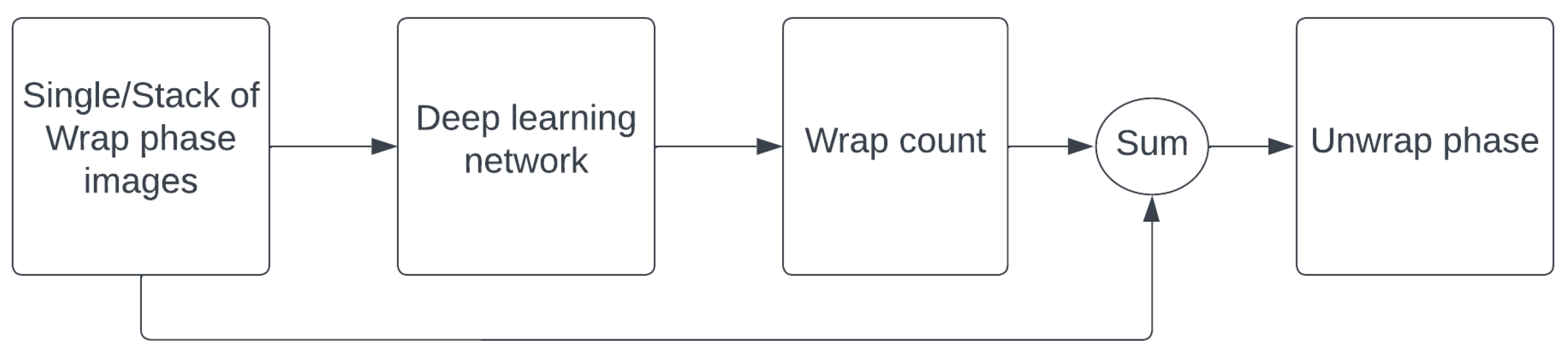
- = wrapped phase, with range [−, ];
- = unwrapped phase;
- k = integer.
1.1. Phase Unwrapping in Single-Baseline Images
Classical Methods to Solve SBPU
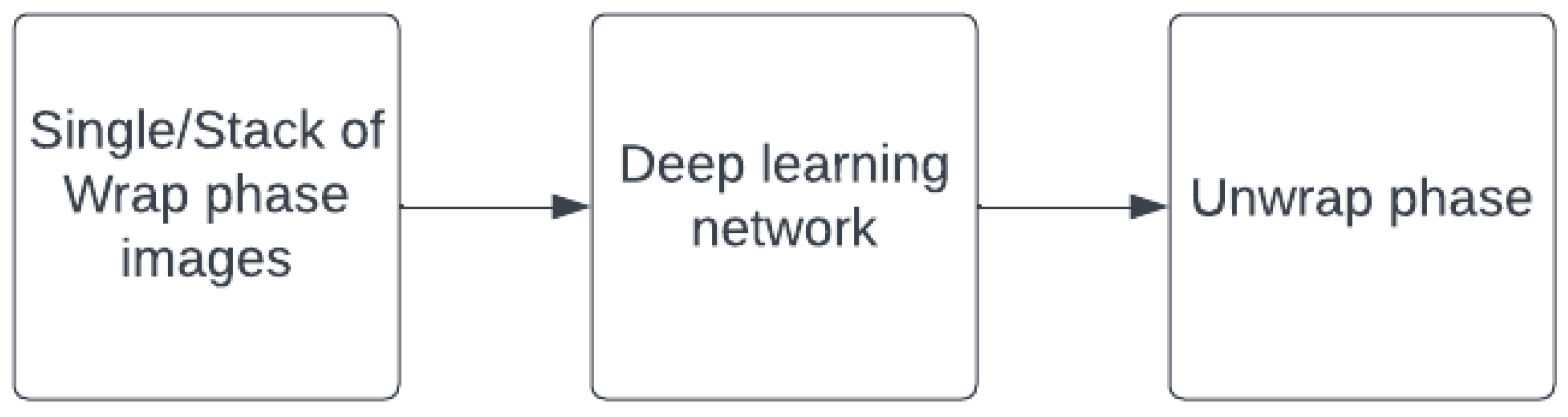
2. Deep Learning for Phase Unwrapping
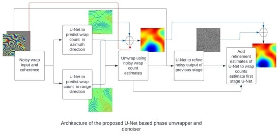
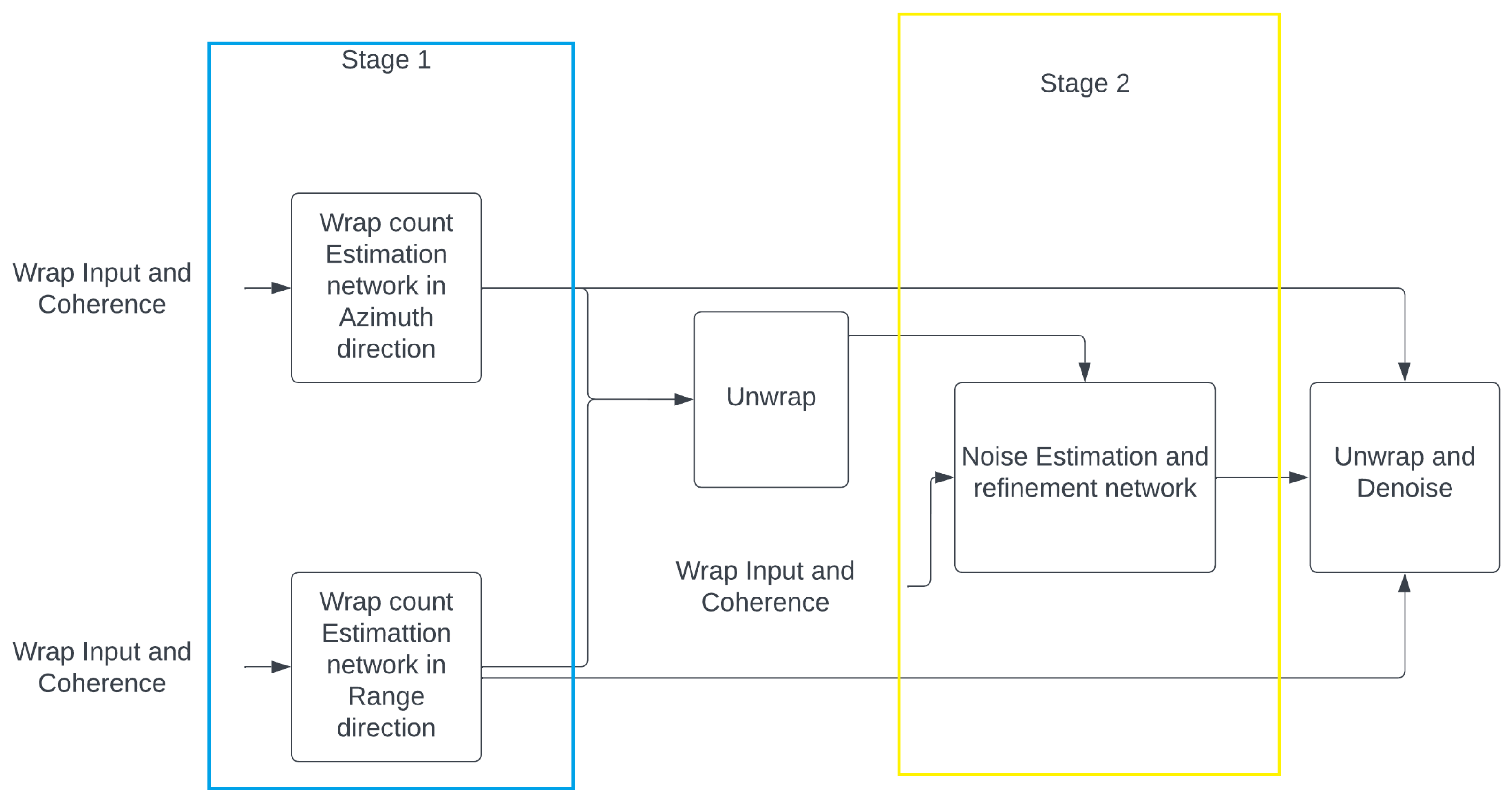
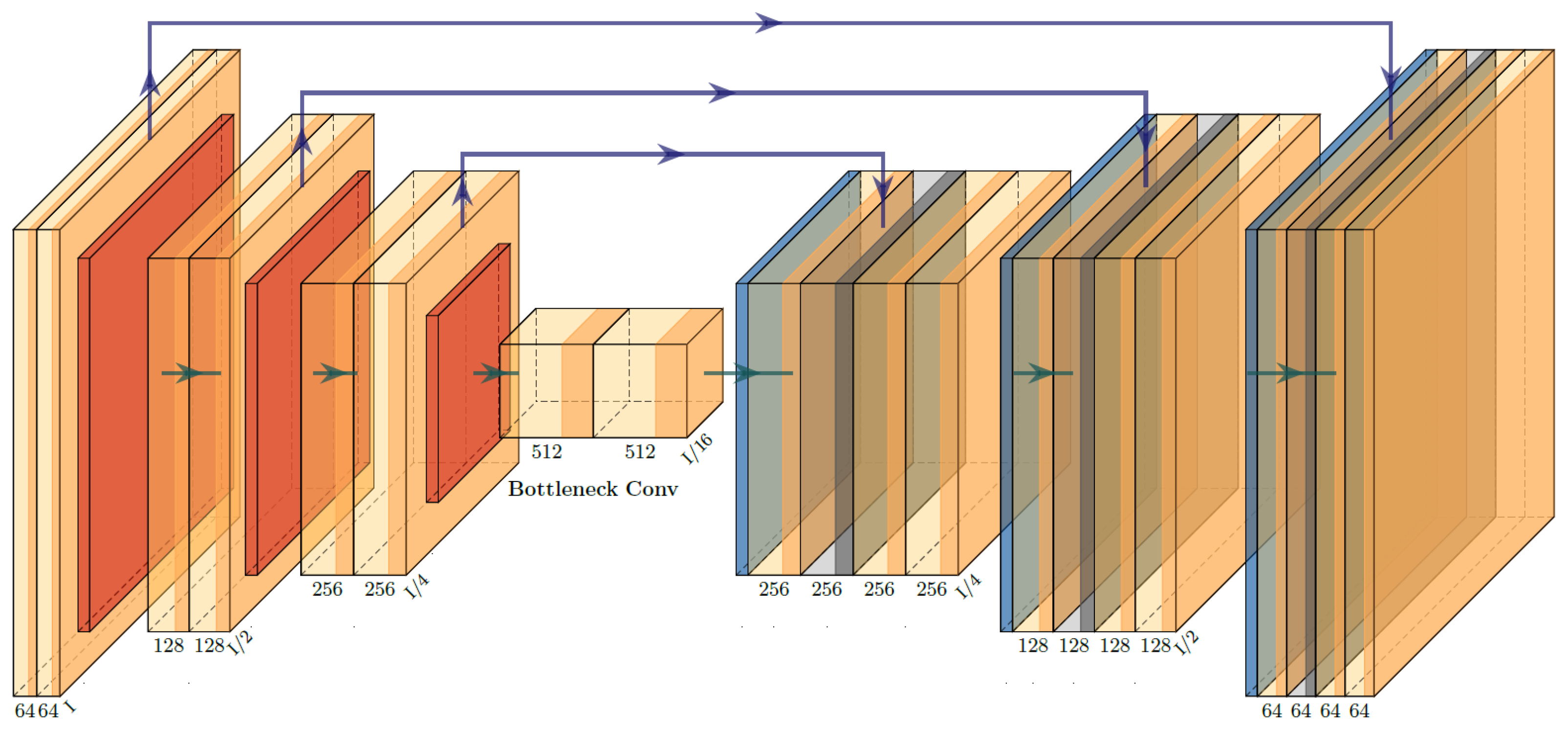
U-Net for Phase Unwrapping
3. Materials and Methods
- r is the refinement factor calculated from the second stage U-Net.
4. Results
- We generate the SLC images S1 and S2 with random Gaussian bubbles as the synthetic motion signals. We make sure that the generated SLCs satisfy Itoh’s condition [6] using a set of control parameters in the simulator.
- We add random additive white Gaussian noise at a random signal level to both SLC images to generate noisy SLC images.
- Using the SLCs, we generate clean and noisy interferometric phases and calculate the ground truth coherence.
- M = height of the interferogram;
- N = width of the interferogram;
- = recovered absolute phase at pixel location [x, y];
- = reference absolute phase at pixel location [x, y].
- X = pixels of a window of the reference absolute phase image;
- Y = pixels of a window of the recovered absolute phase image;
- = mean of the pixel values of window;
- = standard deviation of pixel values of window;
- = cross-correlation of pixels of two windows;
- c = stabilizing factor.
- M = height of the interferogram;
- N = width of the interferogram;
- = recovered absolute phase at pixel location [x, y];
- = reference absolute phase at pixel location [x, y].
5. Discussion
6. Conclusions and Future Work
Author Contributions
Funding
Data Availability Statement
Acknowledgments
Conflicts of Interest
References
- Ferretti, A.; Monti-Guarnieri, A.; Prati, C.; Rocca, F.; Massonet, D. InSAR Principles-Guidelines for SAR Interferometry Processing and Interpretation; ESA Publications: Washington, DC, USA, 2007; Volume 19. [Google Scholar]
- Ng, A.H.M.; Wang, H.; Dai, Y.; Pagli, C.; Chen, W.; Ge, L.; Du, Z.; Zhang, K. InSAR reveals land deformation at Guangzhou and Foshan, China between 2011 and 2017 with COSMO-SkyMed data. Remote Sens. 2018, 10, 813. [Google Scholar] [CrossRef]
- Zhang, S. Absolute phase retrieval methods for digital fringe projection profilometry: A review. Opt. Lasers Eng. 2018, 107, 28–37. [Google Scholar] [CrossRef]
- Dong, J.; Liu, T.; Chen, F.; Zhou, D.; Dimov, A.; Raj, A.; Cheng, Q.; Spincemaille, P.; Wang, Y. Simultaneous phase unwrapping and removal of chemical shift (SPURS) using graph cuts: Application in quantitative susceptibility mapping. IEEE Trans. Med. Imaging 2014, 34, 531–540. [Google Scholar] [CrossRef]
- Ghiglia, D.C.; Pritt, M.D. Two-Dimensional Phase Unwrapping: Theory, Algorithms, and Software; Wiley: Hoboken, NJ, USA, 1998. [Google Scholar]
- Itoh, K. Analysis of the phase unwrapping algorithm. Appl. Opt. 1982, 21, 2470. [Google Scholar] [CrossRef]
- Yu, H.; Lan, Y.; Yuan, Z.; Xu, J.; Lee, H. A Review on Phase Unwrapping in InSAR Signal Processing. IEEE Geosci. Remote Sens. Mag. 2019, 7, 40–58. [Google Scholar] [CrossRef]
- Ghiglia, D.C.; Mastin, G.A.; Romero, L.A. Cellular-automata method for phase unwrapping. J. Opt. Soc. Am. A 1987, 4, 267–280. [Google Scholar] [CrossRef]
- Huntley, J. Noise-immune phase unwrapping algorithm. Appl. Opt. 1989, 28, 3268–3270. [Google Scholar] [CrossRef] [PubMed]
- Goldstein, R.M.; Zebker, H.A.; Werner, C.L. Satellite radar interferometry: Two-dimensional phase unwrapping. Radio Sci. 1988, 23, 713–720. [Google Scholar] [CrossRef]
- Fried, D.L.; Vaughn, J.L. Branch cuts in the phase function. Appl. Opt. 1992, 31, 2865–2882. [Google Scholar] [CrossRef] [PubMed]
- Flynn, T.J. Consistent 2-D phase unwrapping guided by a quality map. In Proceedings of the IGARSS’96, 1996 International Geoscience and Remote Sensing Symposium, Lincoln, NE, USA, 31 May 1996; Volume 4, pp. 2057–2059. [Google Scholar]
- Zhong, H.; Tang, J.; Zhang, S.; Chen, M. An improved quality-guided phase-unwrapping algorithm based on priority queue. IEEE Geosci. Remote Sens. Lett. 2010, 8, 364–368. [Google Scholar] [CrossRef]
- Zhao, M.; Kemao, Q. Quality-guided phase unwrapping implementation: An improved indexed interwoven linked list. Appl. Opt. 2014, 53, 3492–3500. [Google Scholar] [CrossRef]
- Ching, N.H.; Rosenfeld, D.; Braun, M. Two-dimensional phase unwrapping using a minimum spanning tree algorithm. IEEE Trans. Image Process. 1992, 1, 355–365. [Google Scholar] [CrossRef] [PubMed]
- Graham, R.L.; Hell, P. On the history of the minimum spanning tree problem. Ann. Hist. Comput. 1985, 7, 43–57. [Google Scholar] [CrossRef]
- An, L.; Xiang, Q.S.; Chavez, S. A fast implementation of the minimum spanning tree method for phase unwrapping. IEEE Trans. Med. Imaging 2000, 19, 805–808. [Google Scholar] [CrossRef]
- Herráez, M.A.; Burton, D.R.; Lalor, M.J.; Gdeisat, M.A. Fast two-dimensional phase-unwrapping algorithm based on sorting by reliability following a noncontinuous path. Appl. Opt. 2002, 41, 7437–7444. [Google Scholar] [CrossRef]
- Ghiglia, D.C.; Romero, L.A. Minimum Lp-norm two-dimensional phase unwrapping. J. Opt. Soc. Am. A 1996, 13, 1999–2013. [Google Scholar] [CrossRef]
- Costantini, M. A novel phase unwrapping method based on network programming. IEEE Trans. Geosci. Remote Sens. 1998, 36, 813–821. [Google Scholar] [CrossRef]
- Ghiglia, D.C.; Romero, L.A. Robust two-dimensional weighted and unweighted phase unwrapping that uses fast transforms and iterative methods. J. Opt. Soc. Am. A 1994, 11, 107–117. [Google Scholar] [CrossRef]
- Yu, H.; Lan, Y.; Lee, H.; Cao, N. 2-D phase unwrapping using minimum infinity-norm. IEEE Geosci. Remote Sens. Lett. 2018, 15, 1887–1891. [Google Scholar] [CrossRef]
- Yan, Y.; Wang, Y.; Yu, H. An Optimization Model for Two-Dimensional Single-Baseline Insar Phase Unwrapping. In Proceedings of the IGARSS 2022—2022 IEEE International Geoscience and Remote Sensing Symposium, Kuala Lumpur, Malaysia, 17–22 July 2022; pp. 727–730. [Google Scholar]
- Chartrand, R.; Calef, M.T.; Warren, M.S. Exploiting Sparsity for Phase Unwrapping. In Proceedings of the IGARSS 2019—2019 IEEE International Geoscience and Remote Sensing Symposium, Yokohama, Japa, 28 July–2 August 2019; pp. 258–261. [Google Scholar]
- Chen, C.W. Statistical-Cost Network-Flow Approaches to Two-Dimensional Phase Unwrapping for Radar Interferometry; Stanford University: Stanford, CA, USA, 2001. [Google Scholar]
- Nico, G.; Palubinskas, G.; Datcu, M. Bayesian approaches to phase unwrapping: Theoretical study. IEEE Trans. Signal Process. 2000, 48, 2545–2556. [Google Scholar] [CrossRef]
- Xie, X.; Pi, Y. Phase noise filtering and phase unwrapping method based on unscented Kalman filter. J. Syst. Eng. Electron. 2011, 22, 365–372. [Google Scholar] [CrossRef]
- Xie, X.; Li, Y. Enhanced phase unwrapping algorithm based on unscented Kalman filter, enhanced phase gradient estimator, and path-following strategy. Appl. Opt. 2014, 53, 4049–4060. [Google Scholar] [CrossRef]
- Zhang, Y.; Zhang, S.; Gao, Y.; Li, S.; Jia, Y.; Li, M. Adaptive Square-Root Unscented Kalman Filter Phase Unwrapping with Modified Phase Gradient Estimation. Remote Sens. 2022, 14, 1229. [Google Scholar] [CrossRef]
- Martinez-Espla, J.J.; Martinez-Marin, T.; Lopez-Sanchez, J.M. A particle filter approach for InSAR phase filtering and unwrapping. IEEE Trans. Geosci. Remote Sens. 2009, 47, 1197–1211. [Google Scholar] [CrossRef]
- Martinez-Espla, J.J.; Martinez-Marin, T.; Lopez-Sanchez, J.M. An optimized algorithm for InSAR phase unwrapping based on particle filtering, matrix pencil, and region-growing techniques. IEEE Geosci. Remote Sens. Lett. 2009, 6, 835–839. [Google Scholar] [CrossRef]
- Chen, R.; Yu, W.; Wang, R.; Liu, G.; Shao, Y. Integrated denoising and unwrapping of InSAR phase based on Markov random fields. IEEE Trans. Geosci. Remote Sens. 2013, 51, 4473–4485. [Google Scholar] [CrossRef]
- Sarker, I.H. Deep learning: A comprehensive overview on techniques, taxonomy, applications and research directions. SN Comput. Sci. 2021, 2, 420. [Google Scholar] [CrossRef]
- Zhou, L.; Yu, H.; Pascazio, V.; Xing, M. PU-GAN: A One-Step 2-D InSAR Phase Unwrapping Based on Conditional Generative Adversarial Network. IEEE Trans. Geosci. Remote Sens. 2022, 60, 5221510. [Google Scholar] [CrossRef]
- Xu, M.; Tang, C.; Shen, Y.; Hong, N.; Lei, Z. PU-M-Net for phase unwrapping with speckle reduction and structure protection in ESPI. Opt. Lasers Eng. 2022, 151, 106824. [Google Scholar] [CrossRef]
- Wang, Z.; Bovik, A.C.; Sheikh, H.R.; Simoncelli, E.P. Image quality assessment: From error visibility to structural similarity. IEEE Trans. Image Process. 2004, 13, 600–612. [Google Scholar] [CrossRef]
- Zhou, H.; Cheng, C.; Peng, H.; Liang, D.; Liu, X.; Zheng, H.; Zou, C. The PHU-NET: A robust phase unwrapping method for MRI based on deep learning. Magn. Reson. Med. 2021, 86, 3321–3333. [Google Scholar] [CrossRef]
- Qin, Y.; Wan, S.; Wan, Y.; Weng, J.; Liu, W.; Gong, Q. Direct and accurate phase unwrapping with deep neural network. Appl. Opt. 2020, 59, 7258–7267. [Google Scholar] [CrossRef] [PubMed]
- Liu, Y.; Han, Y.; Li, F.; Zhang, Q. Speedup of minimum discontinuity phase unwrapping algorithm with a reference phase distribution. Opt. Commun. 2018, 417, 97–102. [Google Scholar] [CrossRef]
- Spoorthi, G.; Gorthi, R.K.S.S.; Gorthi, S. PhaseNet 2.0: Phase unwrapping of noisy data based on deep learning approach. IEEE Trans. Image Process. 2020, 29, 4862–4872. [Google Scholar] [CrossRef]
- Zhang, J.; Li, Q. EESANet: Edge-enhanced self-attention network for two-dimensional phase unwrapping. Opt. Express 2022, 30, 10470–10490. [Google Scholar] [CrossRef] [PubMed]
- Perera, M.V.; De Silva, A. A joint convolutional and spatial quad-directional LSTM network for phase unwrapping. In Proceedings of the ICASSP 2021—2021 IEEE International Conference on Acoustics, Speech and Signal Processing (ICASSP), Toronto, ON, Canada, 6–11 June 2021; pp. 4055–4059. [Google Scholar]
- Sica, F.; Calvanese, F.; Scarpa, G.; Rizzoli, P. A CNN-based coherence-driven approach for InSAR phase unwrapping. IEEE Geosci. Remote Sens. Lett. 2020. [Google Scholar] [CrossRef]
- Ronneberger, O.; Fischer, P.; Brox, T. U-Net: Convolutional networks for biomedical image segmentation. In Proceedings of the Medical Image Computing and Computer-Assisted Intervention–MICCAI 2015: 18th International Conference, Munich, Germany, 5–9 October 2015; Proceedings, Part III 18. Springer: Cham, Switzerland, 2015; pp. 234–241. [Google Scholar]
- Zhang, T.; Jin, P.J.; Ge, Y.; Moghe, R.; Jiang, X. Vehicle detection and tracking for 511 traffic cameras with U-shaped dual attention inception neural networks and spatial-temporal map. Transp. Res. Rec. 2022, 2676, 613–629. [Google Scholar] [CrossRef]
- Tang, Y.; Huang, Z.; Chen, Z.; Chen, M.; Zhou, H.; Zhang, H.; Sun, J. Novel visual crack width measurement based on backbone double-scale features for improved detection automation. Eng. Struct. 2023, 274, 115158. [Google Scholar] [CrossRef]
- Tang, Y.; Chen, Z.; Huang, Z.; Nong, Y.; Li, L. Visual measurement of dam concrete cracks based on U-net and improved thinning algorithm. J. Exp. Mech. 2022, 37, 209–220. [Google Scholar]
- Tang, Y.; Zhu, M.; Chen, Z.; Wu, C.; Chen, B.; Li, C.; Li, L. Seismic performance evaluation of recycled aggregate concrete-filled steel tubular columns with field strain detected via a novel mark-free vision method. Structures 2022, 37, 426–441. [Google Scholar] [CrossRef]
- Sun, X.; Zimmer, A.; Mukherjee, S.; Kottayil, N.K.; Ghuman, P.; Cheng, I. DeepInSAR—A Deep Learning Framework for SAR Interferometric Phase Restoration and Coherence Estimation. Remote Sens. 2020, 12, 2340. [Google Scholar] [CrossRef]
- Sica, F.; Reale, D.; Poggi, G.; Verdoliva, L.; Fornaro, G. Nonlocal adaptive multilooking in SAR multipass differential interferometry. IEEE J. Sel. Top. Appl. Earth Obs. Remote Sens. 2015, 8, 1727–1742. [Google Scholar] [CrossRef]
- Pu, L.; Zhang, X.; Zhou, Z.; Li, L.; Zhou, L.; Shi, J.; Wei, S. A Robust InSAR Phase Unwrapping Method via Phase Gradient Estimation Network. Remote Sens. 2021, 13, 4564. [Google Scholar] [CrossRef]
- Dabov, K.; Foi, A.; Katkovnik, V.; Egiazarian, K. Image denoising by sparse 3-D transform-domain collaborative filtering. IEEE Trans. Image Process. 2007, 16, 2080–2095. [Google Scholar] [CrossRef] [PubMed]


| Reference | Methodology | Key Highlights | Limitation |
|---|---|---|---|
| Huntley [9] | Minimum length cut algorithm to avoid residues | Works well in high-quality and low-noise phase maps | May not generate output at all if phase maps are too noisy |
| Goldstein [10] | Integration paths encircle an equal number of positive and negative residues | Branch-cut is used to find a solution | NP-Hard |
| Flynn [12], Zhong [13], and Zhao [14] | Quality-maps-guided unwrapping | Coherence was used as measure of quality | Requires many SLCs to generate reliable quality maps |
| Ching et al. [15] | Segmentation-guided unwrapping | Each segment is unwrapped independently | Boundary errors |
| An et al. [17] | Segmentation-guided unwrapping | Faster minimum spanning tree algorithm | Boundary errors |
| Herraez et al. [18] | Reliability-guided unwrapping | Unwraps from most reliable to least reliable pixel | Poor noise immunity |
| Constantine et al. [20] | Lp norm optimization | P = 1, minimum cost problem | Unwrap solution is smooth but not best |
| Ghiglia et al. [21] | Lp norm optimization | P = 2, results in smooth unwrap solution | Affected by noise |
| Chartrand et al. [24] | Sparse optimization | Faster computation | Poor noise immunity |
| SNAPHU [25] | MAP estimation | Captures dependencies with factors such as amplitude | The accuracy depends on the estimates of probability density functions |
| Reference | Network Architecture | Loss Function | Limitation |
|---|---|---|---|
| Zhou et al. [34] | GAN | Adversarial loss | Dataset has no noise |
| Xu et al. [37] | MNet | MAE and SSIM | Only works in low concentration of speckle noise |
| Qin et al. [38] | ResUNet | MAE | Works only in low noise |
| Spoorthly et al. [40] | Dense-UNet | Cross-entropy + Mean absolute error (MAE) | Incorrect unwrapping boundaries |
| Zhang et al. [41] | EESANET | Cross-entropy + L1 loss + residue loss | Poor noise immunity |
| Sica et al. [43] | U-Net | Cross-entropy + Jaccard loss + Mean absolute error (MAE) | Poor noise immunity |
| Perera et al. [42] | Spatial Quad-Directional Long Short-Term Memory (LSTM) | Variance error | Incorrect unwrapping boundaries |
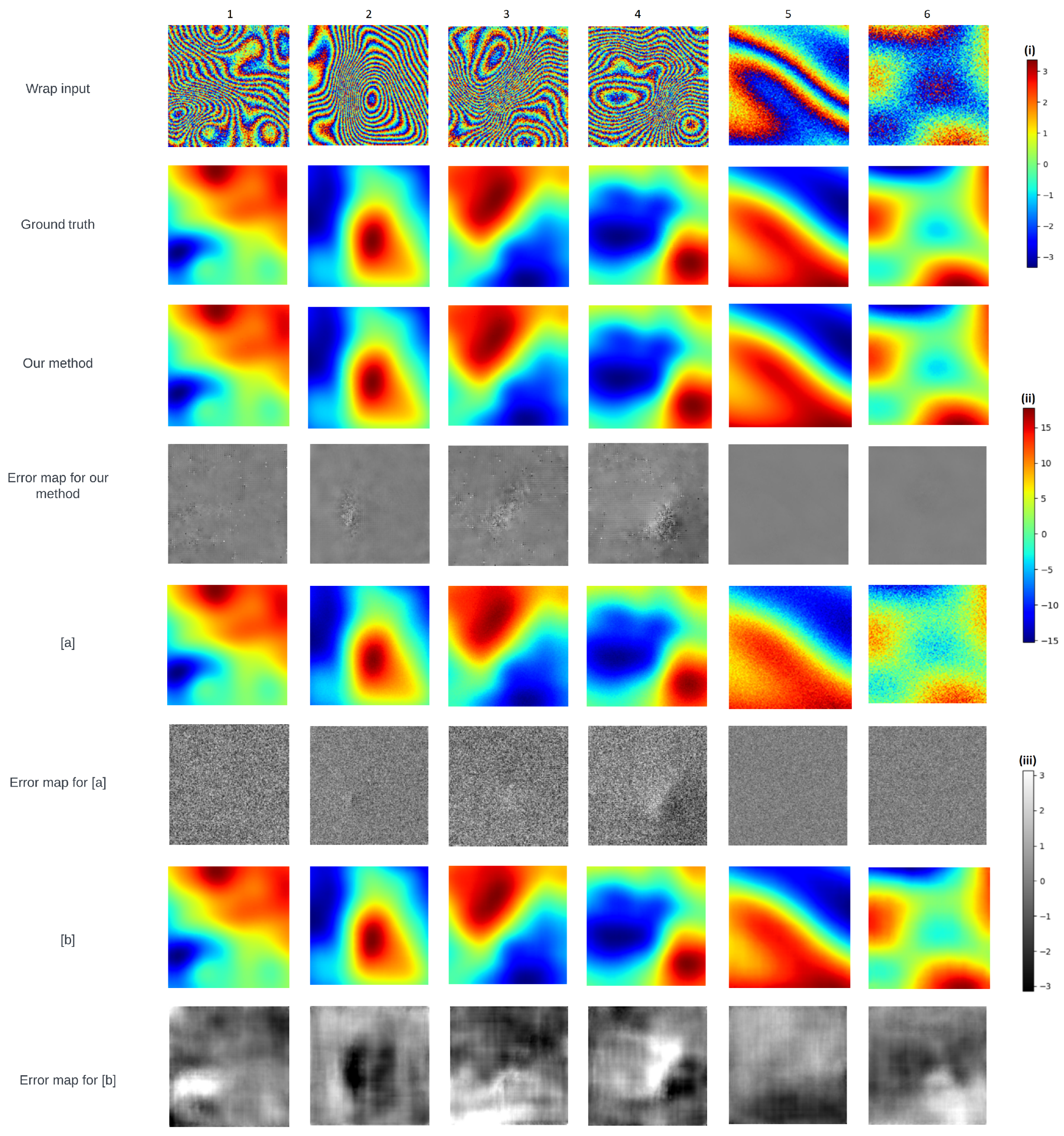
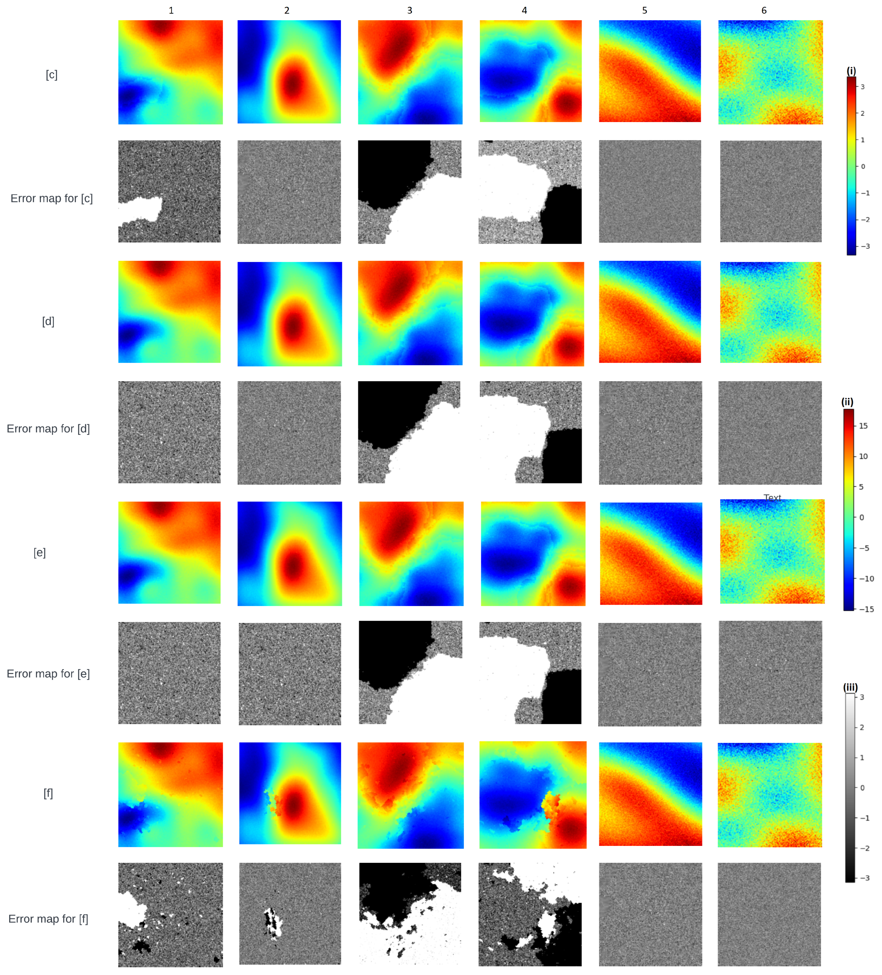
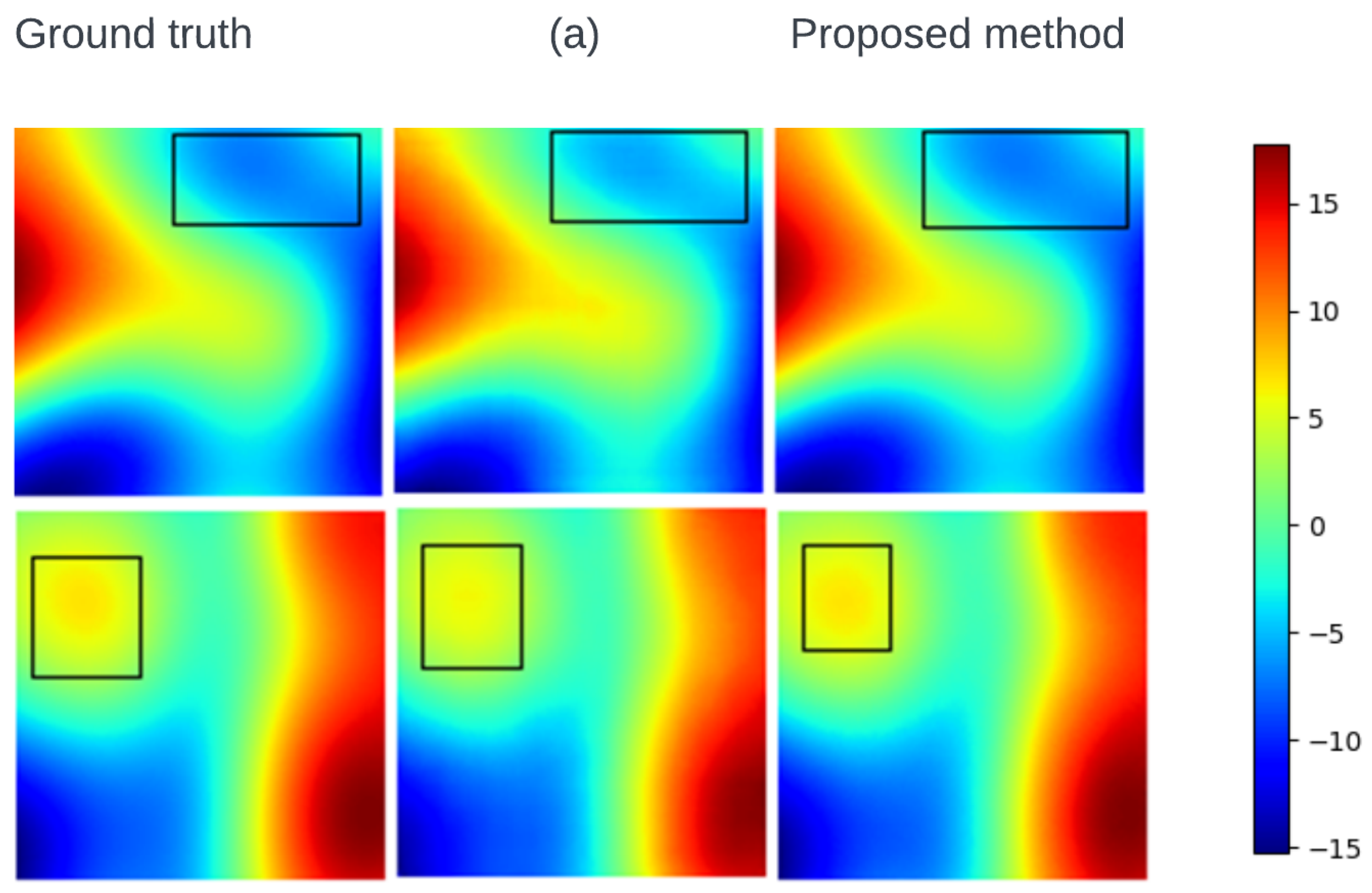
| Method | RMSE (Average/Worst) | SSIM (Average/Worst) | UFR (%) |
|---|---|---|---|
| Herraez et al. [18] | 1.425/9.36 | 0.89/0.33 | 3.52 |
| Chartrand et al. [24] | 0.93/14.12 | 0.93/0.61 | 1.25 |
| SNAPHU [25] | 0.96/12.59 | 0.91/0.63 | 1.2 |
| BM3D [52] + SNAPHU [25] | 0.87/14.69 | 0.93/0.65 | 1.1 |
| Sica et al. [43] | 0.54/2.91 | 0.91/0.64 | 0.01 |
| Perera et al. [42] | 1.01/5.66 | 0.98/0.92 | 0.75 |
| Our method | 0.11/2.18 | 0.99/0.95 | 0.006 |
Disclaimer/Publisher’s Note: The statements, opinions and data contained in all publications are solely those of the individual author(s) and contributor(s) and not of MDPI and/or the editor(s). MDPI and/or the editor(s) disclaim responsibility for any injury to people or property resulting from any ideas, methods, instructions or products referred to in the content. |
© 2023 by the authors. Licensee MDPI, Basel, Switzerland. This article is an open access article distributed under the terms and conditions of the Creative Commons Attribution (CC BY) license (https://creativecommons.org/licenses/by/4.0/).
Share and Cite
Vijay Kumar, S.; Sun, X.; Wang, Z.; Goldsbury, R.; Cheng, I. A U-Net Approach for InSAR Phase Unwrapping and Denoising. Remote Sens. 2023, 15, 5081. https://doi.org/10.3390/rs15215081
Vijay Kumar S, Sun X, Wang Z, Goldsbury R, Cheng I. A U-Net Approach for InSAR Phase Unwrapping and Denoising. Remote Sensing. 2023; 15(21):5081. https://doi.org/10.3390/rs15215081
Chicago/Turabian StyleVijay Kumar, Sachin, Xinyao Sun, Zheng Wang, Ryan Goldsbury, and Irene Cheng. 2023. "A U-Net Approach for InSAR Phase Unwrapping and Denoising" Remote Sensing 15, no. 21: 5081. https://doi.org/10.3390/rs15215081
APA StyleVijay Kumar, S., Sun, X., Wang, Z., Goldsbury, R., & Cheng, I. (2023). A U-Net Approach for InSAR Phase Unwrapping and Denoising. Remote Sensing, 15(21), 5081. https://doi.org/10.3390/rs15215081