Abstract
Land surface temperature (LST) is a fundamental variable of environmental monitoring and surface equilibrium. Although the HJ-1B infrared scanner (IRS) has accumulated many observations, further application of HJ-1B/IRS is limited by the lack of LST products. This study refined the ERA5 atmospheric profile database, instead of the widely used traditional TIGR atmospheric profile database, and simulated the coefficients of the generalized single-channel (GSCs) algorithms to improve LST retrieval. GSCs can be divided into the GSCw and GSCwT algorithms, depending on whether the input is atmospheric water vapor content (WVC) or in situ near-surface air temperature and WVC. Land surface emissivity (LSE) was obtained from the Advanced Spaceborne Thermal Emission and Reflection Radiometer (ASTER) Global Emissivity Dataset (GED) and vegetation/snow cover products. Then, the retrieved LSTs were evaluated using the LSTs from the RTE algorithm, TIGRw/TIGRwT profiles, and in situ near-surface air temperature from the HiWATER experiment in China from 2012 to 2014. The bias (root mean square error (RMSE)) values are displayed as ERA5wT < RTE < ERA5w < TIGRwT < TIGRw. The accuracy of ERA5wT, with a bias (RMSE) of 0.02 K (2.30 K), is higher than that of RTE, with a bias (RMSE) of 0.74 K (2.47 K). The accuracy of RTE is preferable to that of ERA5w, with a bias (RMSE) of 0.89 K (2.48 K), followed by TIGRwT, with a bias (RMSE) of −1.18 K (2.50 K), and then, TIGRw, with a bias (RMSE) of 1.60 K (2.77 K). In summary, the accuracy of LST obtained by GSC from the refined ERA5 atmospheric profiles is higher than that obtained from the TIGR profiles. The accuracy of LST obtained by GSCwT is greater than that obtained by GSCw. The accuracy of LST obtained using in situ near-surface air temperature is higher than that obtained using ERA5 air temperature. The accuracy of LSEASTER is slightly better than that of LSEMOD21. The aforementioned conclusions can provide scientific support to generate HJ-1B/IRS LST products.
1. Introduction
Land surface temperature (LST) is a critical variable in the equilibrium of surface energy [1]. It plays a pivotal role in a number of aspects, including land cover change analysis [2], climate change research [3], vegetation monitoring [4], and the monitoring of agricultural drought [5]. Only satellite remote sensing technology provides the opportunity to obtain LST at a regional or global scale. A number of satellite LST products are frequently widely used at present, covering a spatial scale ranging from 1 km to 100 m, such as the Moderate Resolution Imaging Spectroradiometer (MODIS) [6], Visible Infrared Imaging Radiometer Suite (VIIRS) [7], Advanced Spaceborne Thermal Emission and Reflection Radiometer (ASTER) [8], and Landsat series LST products [9]. These LST products are generated using various retrieval algorithms for LST, such as the single-channel (SC) algorithm [10], split-window (SW) algorithm [6,11], and temperature emissivity separation (TES) algorithm [12].
China’s HJ-1B satellite was launched on 6 September 2008, and it carried an infrared scanner (IRS) with a single thermal infrared channel (spatial resolution: 300 m). Therefore, thermal infrared data of 300 m can be acquired, which have considerable potential in environmental and disaster monitoring. At present, HJ-1B/IRS has accumulated long-term observations. However, its further application is limited by the lack of LST products, since the algorithm for retrieving LST with high accuracy is uncertain. For sensors with a thermal infrared channel, several SC algorithms are already available for LST retrieval, and they are divided into physical and empirical SC algorithms. The former includes the radiative transfer equation (RTE) algorithm [13], while the latter includes the mono-window (MW) algorithm [10] and the generalized single-channel (GSC) algorithm [14]. Windahl and Beurs [15] validated the accuracy of the RTE, MW, and GSC algorithms. The accuracy of these algorithms reduced with a rise in atmospheric water vapor content (WVC). Jiménez-Muñoz et al. [16] proposed the GSC algorithm that used WVC, and the validation outcome indicated root mean square deviations below 1.5 K. Cristóbal et al. [17] improved the algorithm designed by Jiménez-Muñoz [16] by adding near-surface air temperature as an input parameter. The accuracy of the GSC algorithm could be better than 1 K if the WVC was below 2 g/cm2, and the accuracy for retrieving LST could be improved using WVC and near-surface air temperature. Li et al. [13] reported that a composite of the profiles of the National Center for Environmental Prediction and MOD07 can provide higher accuracy than only one type of profile. Pandya et al. [18] used the GSC algorithm for retrieving LST, and the results indicated that the RMSEs of desert and agriculture sites were 1.6 K and 2.7 K, respectively. Wang et al. [19] proposed a method to improve the GSC algorithm based on linear regression, and the validation results showed that the RMSE was 2.767 K. The aforementioned algorithms are mainly applied to Landsat data, but a few are also applied to HJ1B/IRS data. Therefore, it is essential to improve the GSC algorithm for retrieving LST from HJ-1B/IRS data.
Land surface emissivity (LSE) is a critical input variant for SC algorithms. The widely used calculation methods include the normalized difference vegetation index (NDVI) threshold method [20], vegetation cover method (VCM) [21], and classification-based method [22]. Many studies have indicated that classification-based methods may lead to significant uncertainties in estimating barren surface emissivity, further introducing larger errors into LST retrieval [23]. Therefore, enhancing the accuracy of emissivity in desolate surface regions is imperative. In 2014, the National Aeronautics and Space Administration (NASA) published the ASTER Global Emissivity Dataset (GED) [24]. This dataset exhibits excellent accuracy for desolate surfaces [25,26]. Thus, this product has been used to support the retrieval of LST in many satellites, such as MODIS [26], Landsat [14], SLTSR [27], VIIRS [28], and the Advanced Himawari Imager [29]. In the same way, ASTER GEDv3 could be applied to enhance the accuracy of LST retrieval for HJ-1B/IRS.
The current study aims to refine the ERA5 atmospheric profile database, simulate the new coefficients of the GSC algorithms, and improve LST retrieval. This study divides the GSC algorithms into the GSCw and GSCwT algorithms. In GSCw, WVC is input into the GSC algorithm, and its relationships with atmospheric transmittance, upward radiance, and downward radiance are established. In GSCwT, WVC and near-surface air temperature are input into the GSC algorithm, and their relationships with the three aforementioned atmospheric parameters are established. The remainder of this paper is structured as follows. Section 2 provides the data, including remote sensing data, auxiliary data, and ground measurements. Section 3 introduces the methodology, including the LST retrieval algorithm and validation strategy. The results are presented in Section 4. The discussion is found in Section 5, and conclusions are drawn in Section 6.
2. Experimental Data
2.1. Remote Sensing Data
2.1.1. HJ-1B IRS Data
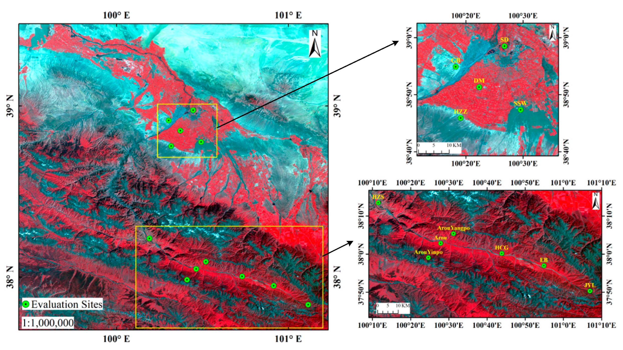
The HJ1-1B satellite was launched in China in September 2008. The payload of HJ-1B includes one IRS, with a thermal infrared band (10.5–12.5 μm), 300 m spatial resolution, and 4-day temporal resolution. This satellite is widely used in disaster warning, ecological environmental protection, and other fields to provide comprehensive environmental monitoring services. This study uses the IRS data of the Heihe River Basin in China (Figure 1) from June 2012 to June 2014 for LST retrieval.
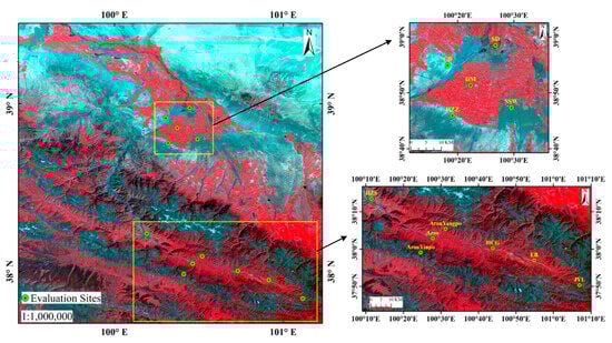
Figure 1.
Spatial location of HiWATER validation sites (map is from HJ-1B CCD false-color composite image).
2.1.2. ASTER GEDv3 Product
The ASTER GEDv3 emissivity product was obtained from ASTER data for clear-sky pixels in the period of 2000 to 2008, and divided into a 1° × 1° grid at 100 m and 1 km spatial resolutions in two forms (HDF5 and binary) [24]. ASTER GEDv3 is used to calculate the bare soil emissivity of IRS. It can be obtained from https://search.earthdata.nasa.gov/search (accessed on 8 October 2022).
2.1.3. ASTER GDEM Product
The ASTER Global Digital Elevation Model (GDEM) v3 gives a global digital elevation model, divided into 1° × 1° tiles of 1/3600 radians, and covering the surface from 83°N to 83°S [30]. This product is used in the elevation interpolation of ERA5 profiles. It can be acquired from https://search.earthdata.nasa.gov/search (accessed on 20 September 2022).
2.1.4. MODIS Product
MCD12Q1 C6 is used to determine land cover types. The product is derived through a supervised decision-tree classification method and can identify 17 land cover types defined by the International Geosphere Biosphere Program (IGBP). MOD10A1 was produced using the daily snow cover detection algorithm and MODIS daily surface reflectance product (MOD09GA). It is used to obtain the dynamic emissivity of snow cover. MOD21A1D C6 is used to verify emissivity accuracy. The MOD21 algorithm is based on the ASTER TES algorithm, combined with improved Water Vapor Scaling (WVS) for atmospheric correction. Their spatial resolutions are 500 m, 500 m, and 1 km, respectively. The temporal resolution is per year, daily, and daily, respectively. MOD10A1 can be acquired from https://nsidc.org/data (accessed on 8 October 2022), while the other data can be obtained from https://ladsweb.modaps.eosdis.nasa.gov/search/ (accessed on 15 October 2022).
2.1.5. Multi-Source Data Synergized Quantitative (MUSYQ) Fractional Vegetation Cover (FVC) Product
The MUSYQ FVC product includes global vegetation cover data and quality control files from 2001 to 2019, with a 500 m spatial resolution and 4-day temporal resolution [31]. It contains 92 pieces of global data per year in HDF5 format with projection information, metadata, etc. The data are generated from the 500 m 4-day MUSYQ Leaf Area Index (LAI) and 500 m 8-day MODIS Clumping Index (CI) products. MUSYQ FVC product is mostly used to obtain the FVC. It can be obtained from http://www.geodata.cn/ (accessed on 12 November 2022).
2.2. Auxiliary Data
2.2.1. ERA5 Atmospheric Reanalysis Data
ERA5 is the latest-generation reanalysis data of the European Centre for Medium-Range Weather Forecasts [32]. ERA5 has single-level and multi-level data. For single-level data, the WVC in ERA5 hourly data on single levels from 1979 to present [32], and 2 m temperature in ERA5-Land hourly data from 1950 to present [33], are used as the input parameters to produce the coefficients of the GSCw and GSCwT algorithms. Multi-level data play two roles. (1) ERA5 profiles are used to set up the refined ERA5 atmospheric profile database, and the database is entered into MODTRAN 5.2 to simulate the coefficients of the GSCw and GSCwT algorithms. (2) The ERA5 profiles with ERA5 hourly data on pressure levels from 1940 to present [32] are used as real-time data to support the RTE algorithm, which can provide 37 layers of profiles from 1000 hPa to 1 hPa. All the aforementioned data are available from https://cds.climate.copernicus.eu/cdsapp#!/home (accessed on 17 October 2022).
2.2.2. TIGR Atmospheric Profile Database
The TIGR atmospheric profile database contains radiosonde data of different seasons from various regions worldwide [34]; it has three versions. TIGR 3 has 2311 atmospheric profiles. Each profile has 43 layers from 1013 hPa to 0.0026 hPa, including longitude, latitude, time, pressure, temperature, WVC, and ozone profiles. The TIGR profiles are used to simulate the coefficients of the GSCw and GSCwT algorithms and validate the accuracy of LST obtained using the refined ERA5 atmospheric profile database.
2.3. Ground Measurements
The Heihe River Basin is situated at 97.1–102.0°E and 37.7–42.7°N. The Heihe Watershed Allied Telemetry Experimental Research (HiWATER) [35] sites are distributed from upstream to downstream of the Heihe River Basin [36]. Considering the high surface heterogeneity of downstream sites, the current study uses observations from seven upstream sites and five midstream sites in the HiWATER experiment to verify the accuracy, covering land types such as the Gobi Desert, sand dunes, desert steppes, wetlands, corn and wheat fields, and alpine meadows. Two major types of equipment are used at the HiWATER sites: SI-111 infrared radiometers and CNR1 net radiometers [37,38]. Table 1 and Figure 1 provide the details and spatial locations of the HiWATER validation sites, respectively.

Table 1.
Details of HiWATER validation sites.
For SI-111 observations, the following formula was used to calculate the LST:
where is the Planck function, is the LST, is the temperature observed using SI-111, is the downward radiation calculated using the SI-111 observed at 55°, and is the SI-111 channel emissivity, obtained from the ground measurements [7].
For the data observed using the CNR1 net radiometer, LST can be given by the following formula:
where is the surface broadband emissivity calculated using the VIIRS broadband emissivity [28], is the LST, and are the upwelling and downwelling long-wave radiation, respectively, and is the Stefan–Boltzmann constant (5.67 × 10⁻⁸ ).
3. Methodology
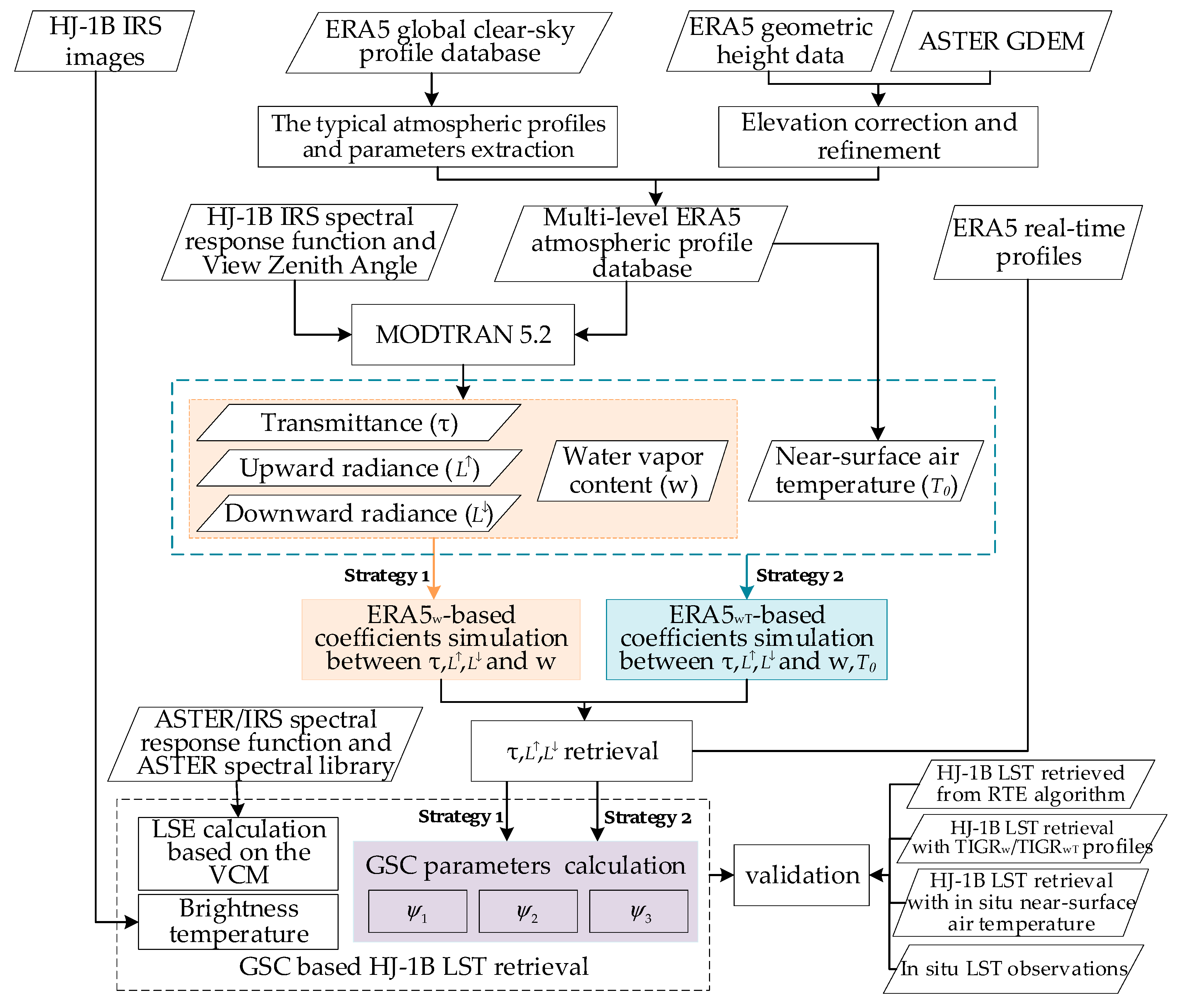
This study refined the ERA5 atmospheric profile database to simulate the coefficients of the GSCw and GSCwT algorithms and improve LST retrieval. LSE was obtained from the ASTER GED and vegetation/snow cover products based on the VCM. Then, the retrieved LSTs were evaluated using the LSTs from the RTE algorithm, TIGRw/TIGRwT profiles, and in situ near-surface air temperature from the HiWATER experiment in China. The flowchart of LST retrieval from HJ-1B/IRS and validation is shown in Figure 2.
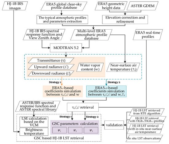
Figure 2.
Flowchart of LST retrieval from HJ-1B/IRS and validation.
3.1. LST Retrieval by the GSC Algorithms
3.1.1. Refined ERA5 Atmospheric Profile Database
We first selected 2457 atmospheric profiles within China from the global clear sky dataset collated by Ermida et al. [39], with longitudes from 74°E to 127°E and latitudes from 19°N to 53°N. Second, the geometric height was downloaded to supplement the database required for the simulation. The above parameters were arranged in the format of tp5 in MODTRAN 5.2. Then, according to the latitude and longitude of each ERA5 atmospheric profile, the same latitude and longitude in ASTER GDEM were matched. Elevation interpolation of geometric height was performed from the ASTER GDEM. It was not performed if the elevation of the ASTER GDEM was lower than the elevation of the first layer of tp5. This method was used to correct and refine the geometric height to improve the accuracy for simulating the coefficients. Finally, the refined ERA5 atmospheric profile database, HJ-1B/IRS spectral response function, and VZA were entered into MODTRAN 5.2 to simulate the coefficients of the GSCw and GSCwT algorithms.
3.1.2. Improved GSCw/GSCwT Algorithm
Jiménez-Muñoz and Sobrino [16] proposed an algorithm for retrieving LST for thermal infrared data. The equations are as follows:
where is the radiance of the sensor, is 1.19104 × 10⁸ , is 14,387.7 μmK, is the sensor’s brightness temperature, is the effective wavelength of the band , and , , and are the atmospheric functions that can be calculated from the following formula:
where and are the atmospheric transmittance and upward radiance in channel at , respectively, and is the downward radiance in channel .
This study refined the ERA5 atmospheric profile database for the simulation of the coefficients of the GSCw and GSCwT algorithms by MODTRAN 5.2. Given the large scanning angle of IRS, the VZA of IRS should be taken into account when simulating coefficients. Due to the range of VZA up to ±33°, 8 VZAs were selected for atmospheric transmittance and upward radiance simulation: 0°, 5°, 10°, 15°, 20°, 25°, 30°, and 35°. For downward radiance, 53° was selected. After inputting 2457 profiles of the multi-level ERA5 atmospheric profile database into MODTRAN 5.2, atmospheric transmittance and upward radiance could be obtained at all angles, and and under a tilt angle exhibited a close linear correlation with and . Then, and could be determined based on and by using a linear function . The expression was obtained as follows:
where denotes and , and denotes and . Table 2 presents the coefficients , all of which have an greater than 0.99.
Table 2.
Coefficients of the unified expression between , and , .
We established the cubic regression formula among , , , and :
where is the WVC, and denotes , , and . Table 3 provides the coefficients . is greater than 0.98.
Table 3.
Regression coefficients of , , , and .
WVC was downloaded for the same time, latitude, and longitude of the IRS image and input into Formula (8) to obtain , , and . Then, and were input into Formula (7) to obtain and . Finally, , , and were input into Formula (6) to obtain the atmospheric functions (AFs), which were further input into Formula (3) to obtain the LST. This method of inputting WVC into the GSCw algorithm coefficients obtained from the ERA5 profiles is denoted as ERA5w.
Cristóbal et al. [17] determined that the accuracy for LST retrieval can be improved using WVC and near-surface air temperature. We established the binary quadratic nonlinear regression among WVC, near-surface air temperature, , , and . The regression formula is as follows:
where is the WVC, is the near-surface air temperature, the simulation uses the temperature of the first layer of the profile, and denotes , , and . Table 4 presents the coefficients , all of which have an greater than 0.98.
Table 4.
Regression coefficients of , T0, , , and .
The process of inputting WVC and 2 m temperature into the GSCwT algorithm coefficients obtained from the ERA5 profiles is referred to as ERA5wT.
3.1.3. LSE Calculation
LSE is calculated using the VCM, which assumes that each pixel is composed of bare soil and vegetation, and the formula is as follows:
where , , and are the emissivity of each pixel, vegetation, and bare soil, respectively. is the fractional vegetation cover of each pixel, and is the cavity term, which can be given by the following formula:
where is the shape factor, which depends on the height of vegetation and the distance between elements on the surface [40].
Li et al. [26] used the ASTER GEDv3 product to calculate the LSE of MODIS SW channels, and this method was also used to obtain the LSE of IRS. The land surface was divided into bare soil and vegetation, snow and ice, inland water, and wetland. The bare soil emissivity of ASTER 13 and 14 was obtained and normalized to the bare soil emissivity of IRS 4. Bare soil emissivity can be obtained using the following equation:
where and are the bare soil and ASTER GEDv3 emissivity, respectively; is the vegetation emissivity, which is obtained using the vegetation emissivity in the ASTER spectral library [41] combined with the ASTER spectral response function; and is calculated using the mean from ASTER GEDv3.
In Equation (13), , , and denote the mean, minimum, and maximum values of ASTER GEDv3, respectively.
The linear regression formula of ASTER 13 and 14 and IRS 4 emissivity was obtained with an RMSE of 0.00611 and of 0.98, indicating high accuracy.
where , , and are the bare soil emissivity of IRS 4, ASTER 13, and 14, respectively.
Vegetation types were determined based on land surface types, and each vegetation emissivity was calculated using the MCD12Q1 product and vegetation emissivity in the ASTER spectral library. Table 5 provides the vegetation emissivity of IRS and shape factor F for different vegetation types. is the bare soil and vegetation emissivity, which can be obtained using Formula (10), and is calculated using the MUSYQ FVC product.
Table 5.
Vegetation emissivity of IRS and shape factor F for different vegetation types.
The proportion of inland water and wetland is small, and its emissivity is stable. Therefore, water and wetland emissivity were calculated using MCD12Q1, the IRS spectral response function, and water and wetland emissivity in the ASTER spectral library. Their emissivity values were assigned as 0.989 and 0.985, respectively. For snow and ice, some covers are permanent, while others are only covered in winter. Hence, dynamic changes must be considered, and MOD10A1 is frequently used to calculate dynamic emissivity.
where is bare soil and vegetation emissivity, is the snow cover fraction obtained by MOD10A1, and is the snow and ice emissivity calculated with snow and ice emissivity in the ASTER spectral library and IRS spectral response function, which is 0.984. is the final IRS emissivity. This method for calculating LSE is labeled as LSEASTER.
3.2. Validation Strategy
The retrieved HJ-1B/IRS LSTs were evaluated using the ground-measured LSTs via the temperature-based verification method, and were also validated using the LSTs retrieved from the RTE algorithm, TIGRw/TIGRwT profiles, and in situ near-surface air temperature from the HiWATER experiment in China. To eliminate the effect of thin clouds on the validation consequence, the “3σ-Hampel identifier” was first utilized to eliminate anomalies [23]; then, the bias and RMSE were used to evaluate the accuracy of the filtered LST.
3.2.1. HJ-1B LST Retrieved from RTE Algorithm
The ERA5 atmospheric profiles are widely used for the RTE algorithm. This section verifies whether the refined ERA5 atmospheric profile database performs well in the GSC algorithm. Based on RTE, the at-sensor radiance of the channel below a clear sky atmosphere can be obtained as [13]:
where is the LST, is the VZA, is the brightness temperature in channel , is the blackbody radiance in channel , is the LSE in channel at , and are the atmospheric transmittance and upward radiance in channel at , respectively, and is the downward radiance in channel .
The RTE algorithm uses ERA5 real-time atmospheric profiles as input data. First, the ERA5 atmospheric profile of 37 layers was extracted and elevation interpolation was carried out. Then, linear interpolation was conducted for pressure, temperature, and other atmospheric parameters, and spatial interpolation was performed using the four grid points. Finally, time interpolation was achieved using two Coordinated Universal Times around the time of HJ-1B/IRS. The influence of VZA was considered when the interpolated profiles were entered into MODTRAN 5.2. For atmospheric transmittance and upward radiance, the VZA of the IRS images was read using the latitude and longitude of each ERA5 profile. For downward radiance, 53° was selected as the VZA instead of the hemispheric value [42]. , , and were combined with LSE to calculate the LST. The bias and RMSE between the RTE LST and in situ LST were calculated to support accuracy verification.
3.2.2. HJ-1B LST Retrieval with TIGRw/TIGRwT Profiles
The widely used traditional TIGR3 atmospheric profile database is static. This study verifies whether the refined ERA5 atmospheric profile database can improve LST retrieval by the GSC algorithm compared with the TIGR atmospheric profiles. The same simulation method as the ERA5 database was used to obtain the GSCw and GSCwT algorithm coefficients by using the TIGR atmospheric profiles. Table 6, Table 7 and Table 8 present the coefficients ; ; and in Equations (7)–(9). The method of inputting WVC into the GSCw algorithm coefficients obtained from the TIGR profiles is denoted as TIGRw. TIGRwT involves inputting the WVC and 2 m temperature into the GSCwT algorithm coefficients obtained from the TIGR profiles. Finally, the bias and RMSE between the TIGRw/TIGRwT LST and in situ LST were calculated to support accuracy verification.
Table 6.
Expression coefficients between , and , from TIGR profiles.
Table 7.
Regression coefficients of , , , and from TIGR profiles.
Table 8.
Regression coefficients of , T0, , , and from TIGR profiles.
3.2.3. HJ-1B LST Retrieval with In Situ Near-Surface Air Temperature
In GSCwT, the 2 m temperature was used as the near-surface air temperature with a coarse spatial resolution. This section aims to explore whether in situ near-surface air temperature can improve LST retrieval by the GSCwT algorithm. This temperature was calculated from the automatic weather stations of the HiWATER experiment. The air temperature sensor was set up at 5 m. The in situ near-surface air temperature was input into the GSCwT algorithm, and the outcomes of the LST retrievals were extracted using the location of ground observations. Finally, the bias and RMSE between the IRS LSTs using the 2 m temperature and in situ near-surface air temperature were used to support accuracy verification.
4. Results
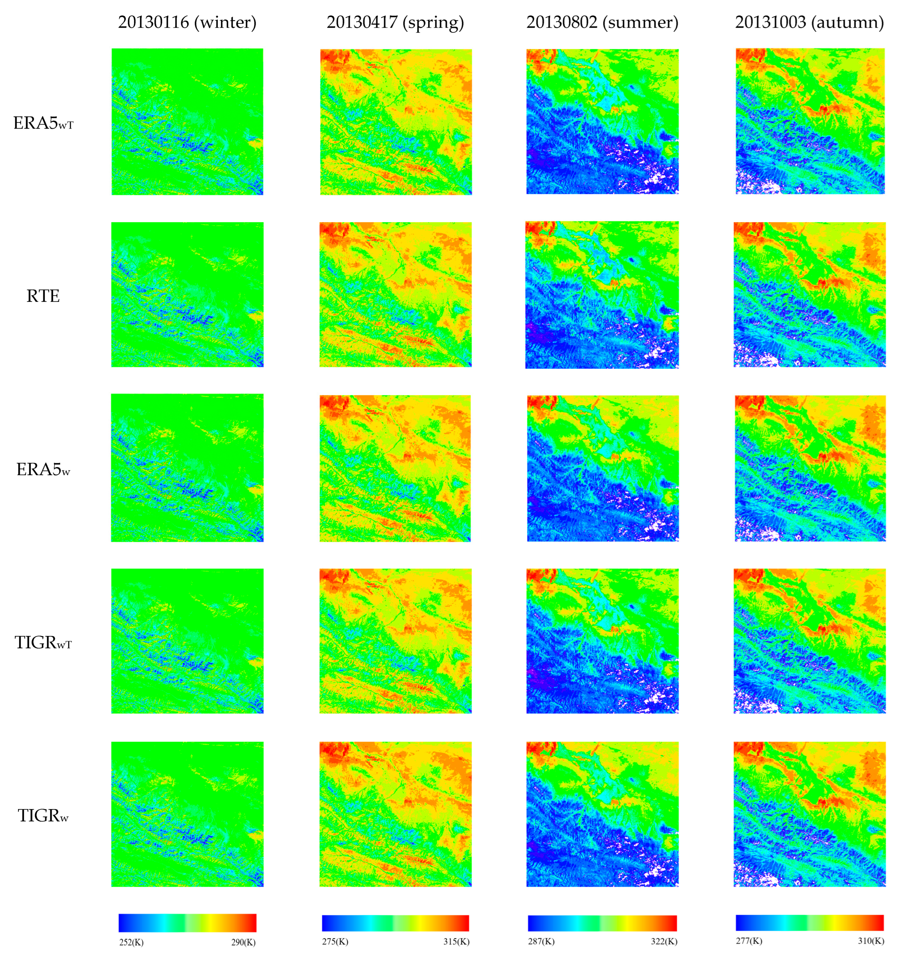
We chose the LST retrieval results for one day in each season to show the comparisons among IRS LSTs derived from ERA5wT, RTE, ERA5w, TIGRwT, and TIGRw in Figure 3. The LSTs of ERA5wT, ERA5w, RTE, and TIGRwT are higher than that of TIGRw in autumn in the oasis situated in the northwest of the basin, while the LSTs of the bare soil part located in the northwest and midstream of the basin are less than those from TIGRw. The bias of TIGRw is higher than that of ERA5wT, ERA5w, RTE, and TIGRwT. During winter, the TIGRw-derived LST map shows more pixels covered by bare soil than other LST maps produced using ERA5wT, ERA5w, RTE, and TIGRwT. This is consistent with the variations in spring and summer.
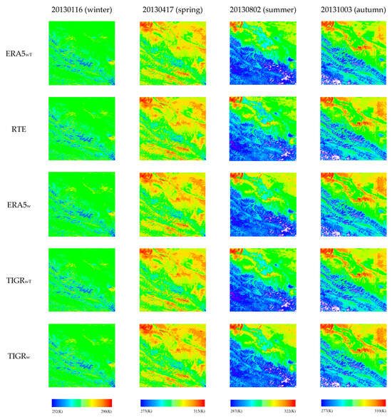
Figure 3.
Comparisons among IRS LSTs derived from ERA5wT, RTE, ERA5w, TIGRwT, and TIGRw.
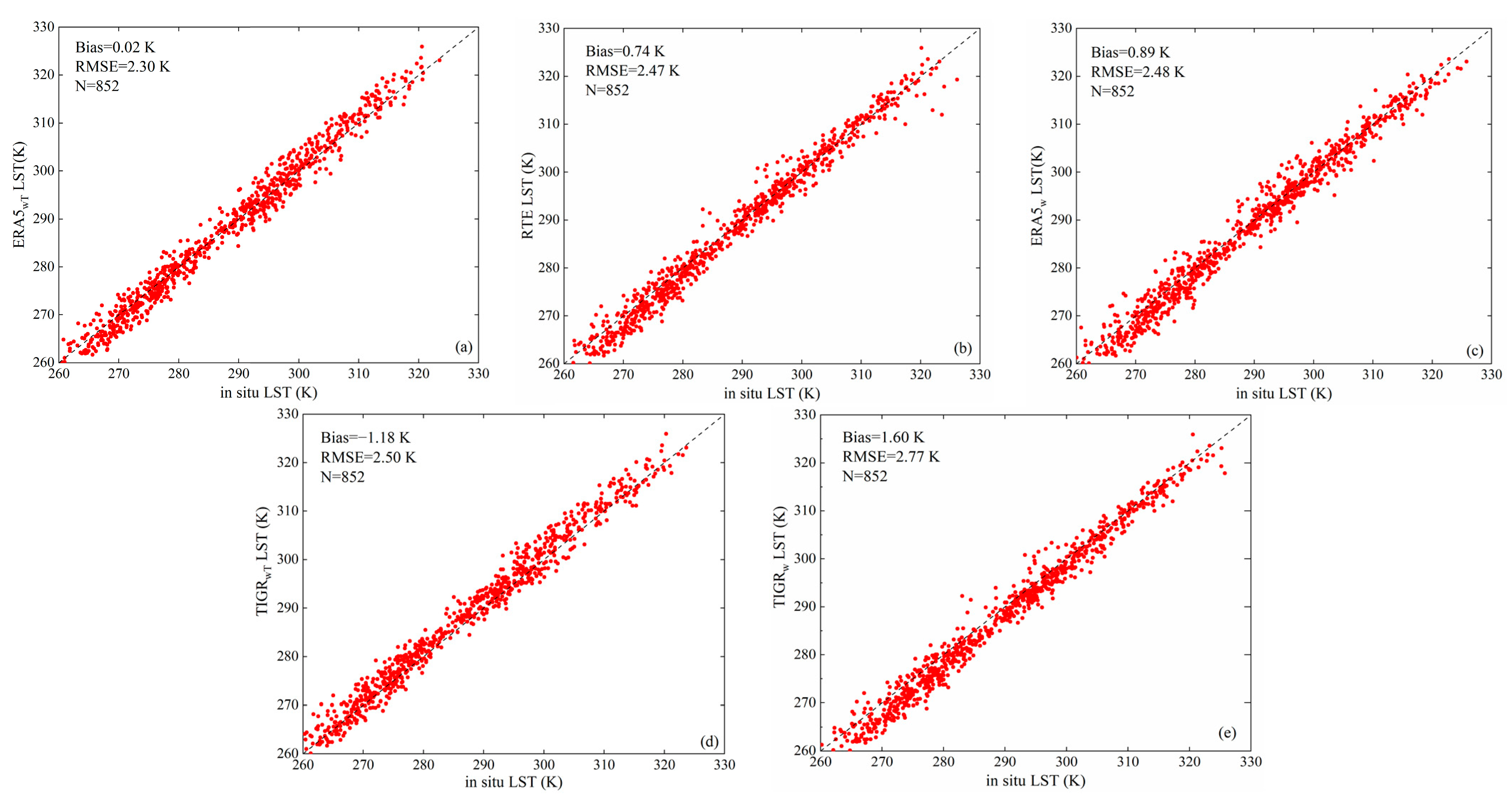
After cloud screening and the removal of outliers, Figure 4 displays scatterplots comparing the IRS and in situ LSTs at 12 HiWATER sites. The number of IRS in situ LST pairs is 852. The bias (RMSE) values are organized as ERA5wT < RTE < ERA5w < TIGRwT < TIGRw. The accuracy of ERA5wT, with a bias (RMSE) of 0.02 K (2.30 K) is higher than that of RTE, with a bias (RMSE) of 0.74 K (2.47 K). The accuracy of RTE is preferable to that of ERA5w, with a bias (RMSE) of 0.89 K (2.48 K), followed by TIGRwT, with a bias (RMSE) of −1.18 K (2.50 K), and then, TIGRw, with a bias (RMSE) of 1.60 K (2.77 K). The accuracy of the GSC algorithm is close to that of the RTE algorithm, probably because the study area is semi-arid and WVC is low, leading to the high accuracy of the GSC algorithm. The validation consequence indicates that ERA5wT exhibits the highest accuracy.
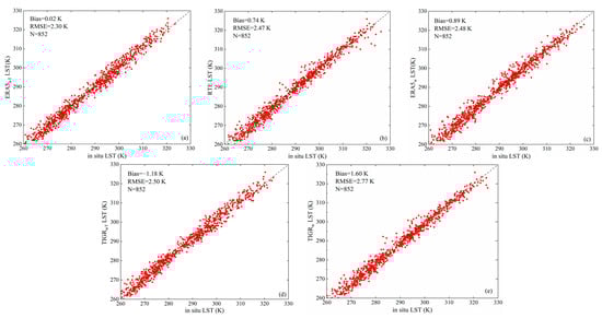
Figure 4.
Scatterplots comparing IRS and in situ LSTs at 12 HiWATER sites. (a) ERA5wT LST. (b) RTE LST. (c) ERA5w LST. (d) TIGRwT LST. (e) TIGRw LST.
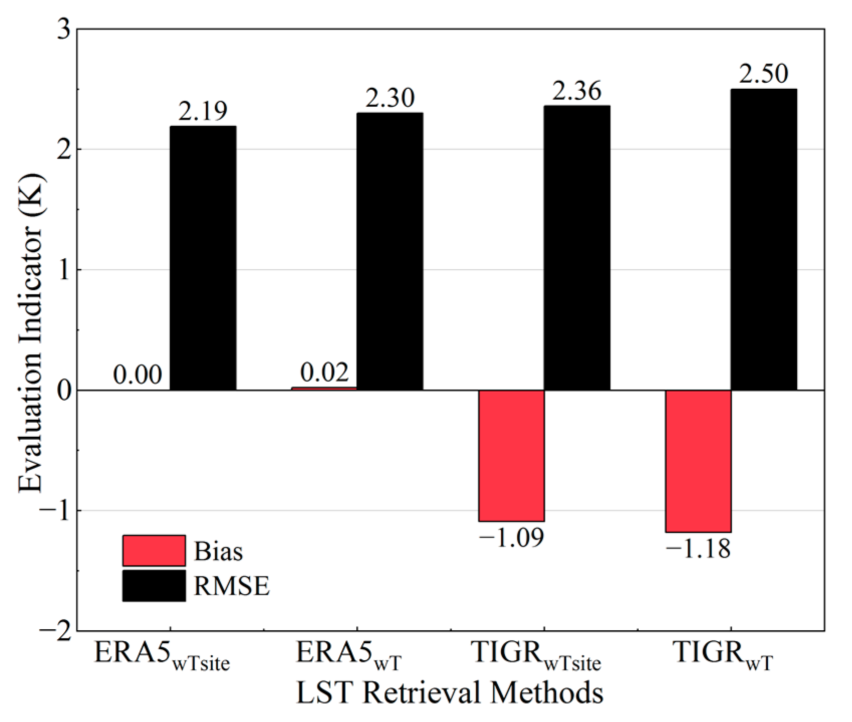
In GSCwT, we used the ERA5 near-surface air temperature and in situ near-surface air temperature, and Figure 5 displays the bias and RMSE of the IRS LSTs. The bias (RMSE) values are listed as ERA5wTsite < ERA5wT < TIGRwTsite < TIGRwT. The accuracy of ERA5wTsite, with a bias (RMSE) of 0 K (2.19 K) is higher than that of ERA5wT, with a bias (RMSE) of 0.02 K (2.30 K). The accuracy of ERA5wT is preferable to that of TIGRwTsite, with a bias (RMSE) of −1.09 K (2.36 K), followed by TIGRwT, with a bias (RMSE) of −1.18 K (2.50 K). Compared with those of ERA5wT, the bias and RMSE of ERA5wTsite decreased by 0.02 K and 0.11 K, respectively. Compared with those of TIGRwT, the bias and RMSE of TIGRwTsite reduced by 0.09 K and 0.14 K, respectively. The accuracy of LST calculated via in situ near-surface air temperature is higher than that calculated via ERA5 near-surface air temperature, because in situ near-surface air temperature was calculated from the automatic weather stations of the HiWATER experiment, which is more accurate than ERA5 near-surface air temperature. Therefore, in situ near-surface air temperature affects the LSTs retrieved by the GSCwT algorithm.
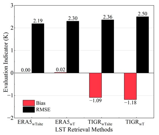
Figure 5.
Bias and RMSE of IRS LSTs using ERA5 near-surface air temperature and in situ near-surface air temperature.
5. Discussion
5.1. Effect of Site, Month, WVC, and VZA on LST Retrieval
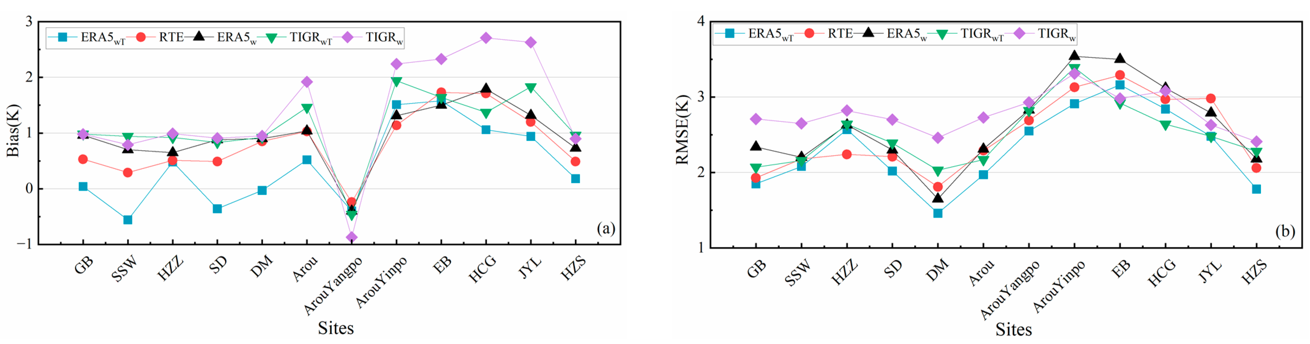
To explore the effect of site on LST retrieval more intuitively, Figure 6 displays the bias and RMSE of the IRS LSTs at different sites. Table 9 indicates the validation consequences for IRS LSTs at 12 HiWATER sites. The accuracy of ERA5wT, ERA5w, RTE, TIGRwT, and TIGRw varies consistently at different sites. The bias (RMSE) of ERA5wT varies from −0.56 K (1.46 K) to 1.58 K (3.16 K), with a mean value of 0.02 K (2.30 K). The bias (RMSE) of ERA5w changes from −0.40 K (1.65 K) to 1.79 K (3.50 K), with an average of 0.89 K (2.48 K). The bias (RMSE) of RTE changes from −0.24 K (1.81 K) to 1.73 K (3.29 K), with an average of 0.74 K (2.47 K). The bias (RMSE) of TIGRwT varies from −0.46 K (2.03 K) to 1.94 K (3.39 K), with a mean value of −1.18 K (2.50 K). The bias (RMSE) of TIGRw changes from −0.92 K (2.41 K) to 2.71 K (3.31 K), with an average of 1.60 K (2.77 K).
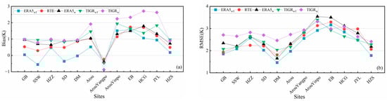
Figure 6.
Bias and RMSE of IRS LSTs at different sites. (a) Bias of sites. (b) RMSE of sites.
Table 9.
Validation results for IRS LSTs at 12 HiWATER sites.
The sites cover a variety of land types, such as sand dunes, wetlands, desert steppe, Gobi Desert, corn fields, and alpine meadows. Obviously, ERA5wT and ERA5w achieve the best accuracy on DM, with RMSEs of 1.46 K and 1.65 K, respectively. ERA5wT exhibits the best accuracy on HZS, with an RMSE of 1.78 K. The land types of DM and HZS are corn and wheat fields, respectively. The LSEASTER in this study exhibits good accuracy on GB, SSW, and HZZ. These outcomes indicate that the accuracy of retrieving LST can be enhanced by using the physically retrieved ASTER GED product, particularly on barren surfaces. The sites Arou, ArouYinpo, EB, HCG, and JYL exhibit overestimation, with a bias greater than 1K, while all the other sites have a bias within 1K, particularly on SSW and SD, obtaining better consequences. Only three sites (ArouYinpo, EB, and HCG) have an RMSE greater than 3 K. For ERA5wT, ERA5w, and RTE, the RMSE of the five upstream sites (ArouYangpo, ArouYinpo, EB, HCG, and JYL) is higher than the average RMSE. The complex topography and large spatial heterogeneity of upstream sites lead to the overestimation of LST.
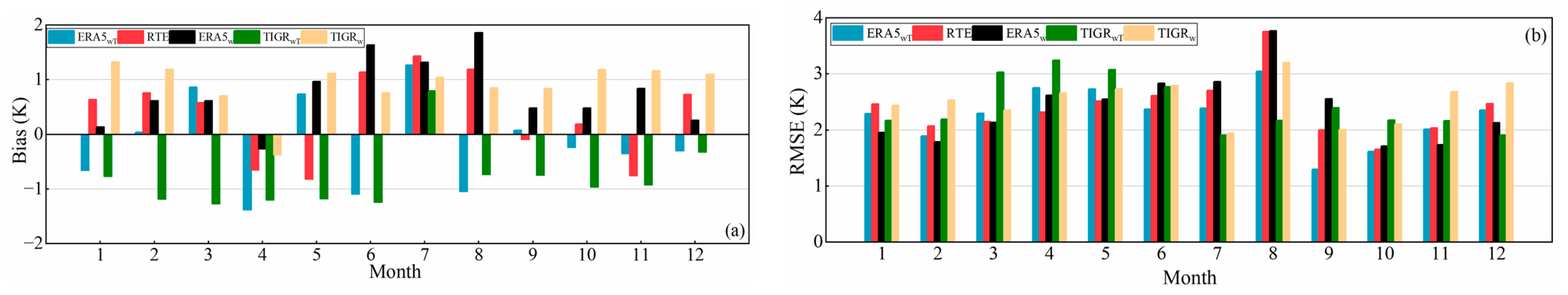
We further analyzed monthly changes in the results of the IRS LSTs. Figure 7 displays the bias and RMSE of IRS LSTs in different months. The RMSEs are generally small during autumn and winter and large during spring and summer. The results show that during autumn and winter, air temperature and humidity are low, and the LST tends to be at a low value. WVC is low, and the LST retrieval error is small. During spring and summer, the LST changes significantly with high WVC. During summer, clouds appear frequently, which reduces valid observations, which may lead to a large bias and RMSE of the results. In summary, the atmospheric characteristics and amount of data exert essential effects on LST retrieval, and these factors should be fully considered during LST retrieval.
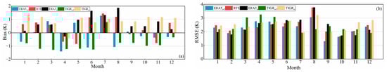
Figure 7.
Bias and RMSE of IRS LSTs in different months. (a) Bias of sites. (b) RMSE of sites.
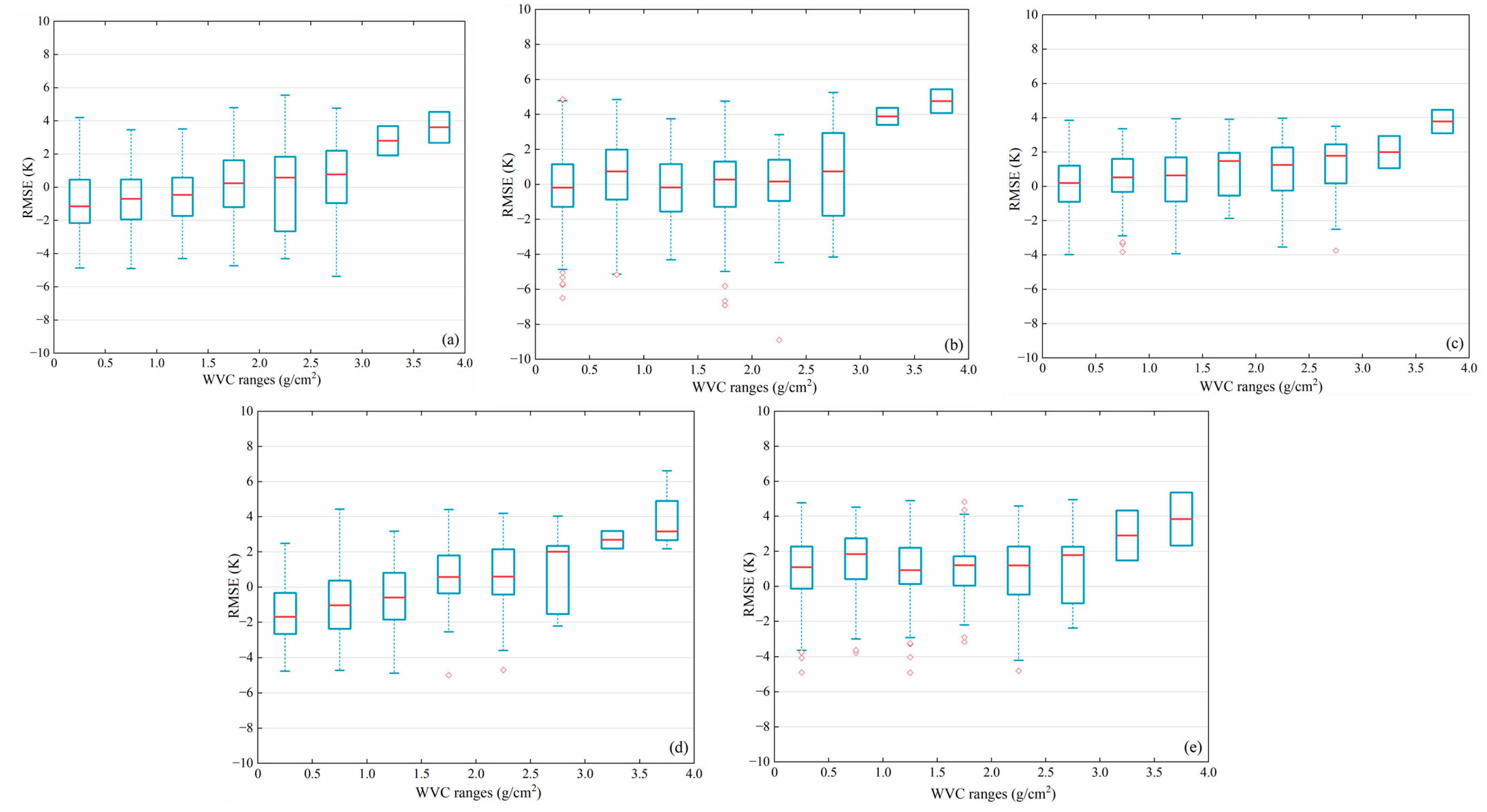
To explore the influence of WVC on the LST retrieval results, the WVCs were divided into eight groups: [0, 0.5], [0.5, 1], [1, 1.5], [1.5, 2], [2, 2.5], [2.5, 3], [3, 3.5], and [3.5, 4]. Figure 8 shows the RMSE of the IRS LSTs in eight groups of WVCs. The RMSEs of the five methods increase with a rise in WVC. All the RMSEs are below 3 K for WVC at 0–3 g/cm2, and the change increases sharply when WVC is larger than 3 g/cm2. The RMSEs of RTE and TIGRw for WVC at 0.5–1.0 g/cm2 are slightly larger than that for WVC at 1.0–1.5 g/cm2, and no significant difference is found in the RMSEs for WVC at 1.0–2.5 g/cm2. Notably, the bias of RTE at low WVCs is the smallest and close to 0. An underestimation of ERA5wT and TIGRwT occurs by nearly 2 K, and an overestimation of ERA5w and TIGRw occurs by nearly 1 K. At high WVCs, the variance of errors produced by TIGRwT is the smallest, while that of ERA5w is the largest. The reason for such a phenomenon is that the atmospheric correction error is large when WVC is high, and consequently, the LST error is large. In summary, the GSC method exhibits excellent accuracy at small WVCs, which is in accordance with Jimenez-Munoz et al. [17].
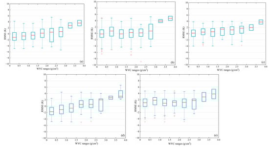
Figure 8.
RMSE of IRS LSTs in eight groups of WVCs. (a) RMSE of ERA5wT. (b) RMSE of RTE. (c) RMSE of ERA5w. (d) RMSE of TIGRwT. (e) RMSE of TIGRw.
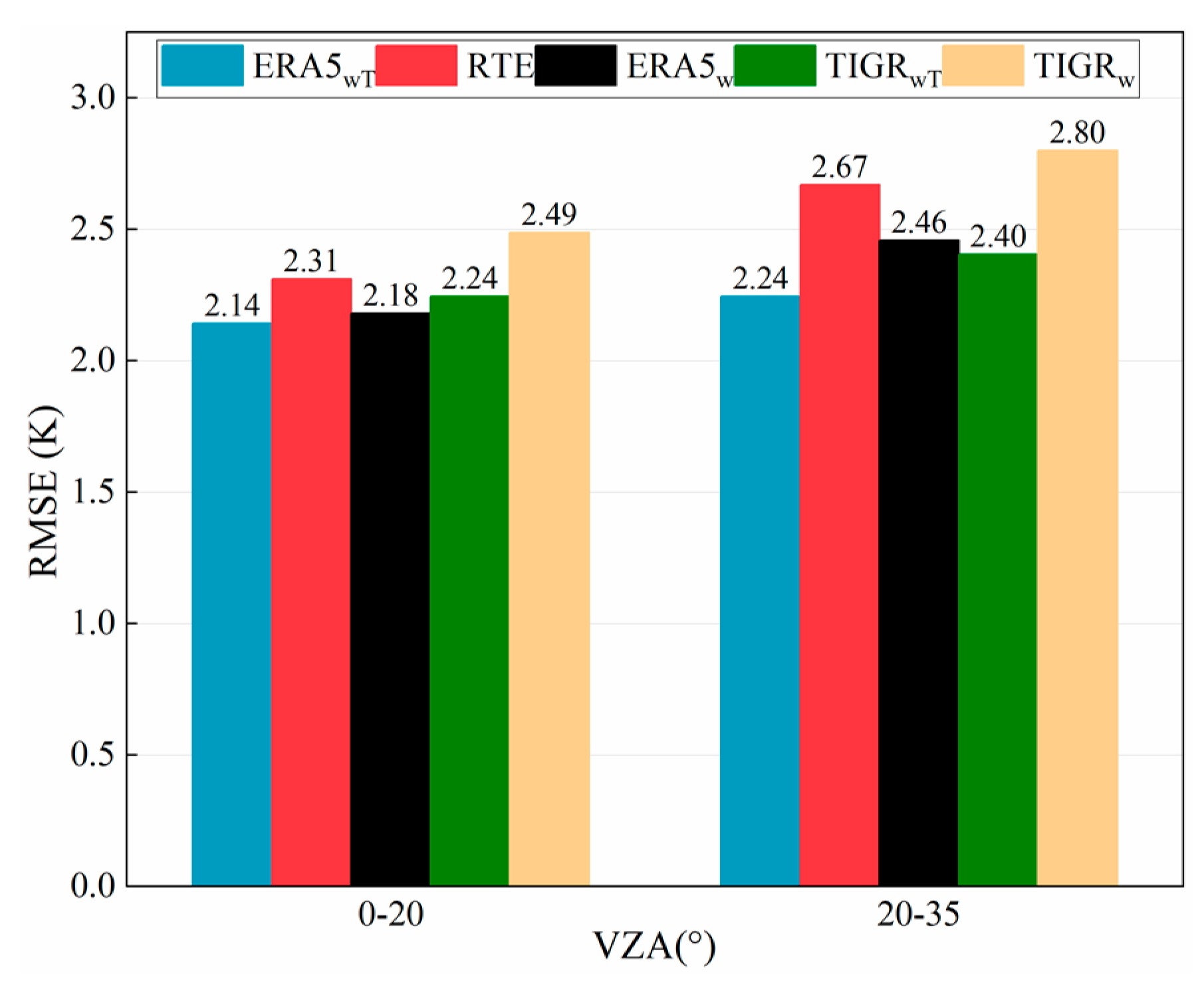
The VZA of HJ-1B/IRS can reach ±33°. To find out the connection between LST errors and VZAs, the VZAs were divided into two groups: [0–20°] and [20–35°]. Figure 9 presents the RMSE of IRS LSTs in the two groups of VZAs. The consequence demonstrates that the RMSEs increase as VZA increases, and the RMSEs are all less than 3 K. The RMSE of ERA5wT rises by 0.10 K from [0–20°] to [20–35°], and ERA5w increases by 0.28 K, followed by an increase of 0.16 K for TIGRwT; then, TIGRw rises by 0.31 K, while RTE exhibits the largest change of 0.36 K. These results demonstrate that the larger the VZA, the longer the path observed by the sensor, and the more pronounced the atmospheric effect, and thus, the larger the LST error. This effect is more evident for satellite sensors with large VZAs, such as MODIS [7,26]. In addition, VZA can also cause differences between the target range obtained by satellite sensors and ground measuring instruments. In summary, the effect of VZA must be considered when obtaining LST products.
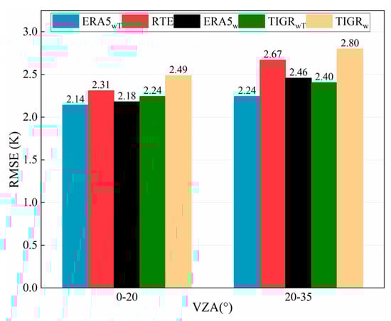
Figure 9.
RMSE of IRS LSTs in two groups of VZAs.
5.2. Effect of Different LSE Data on LSTs Retrieved by the GSC Algorithm
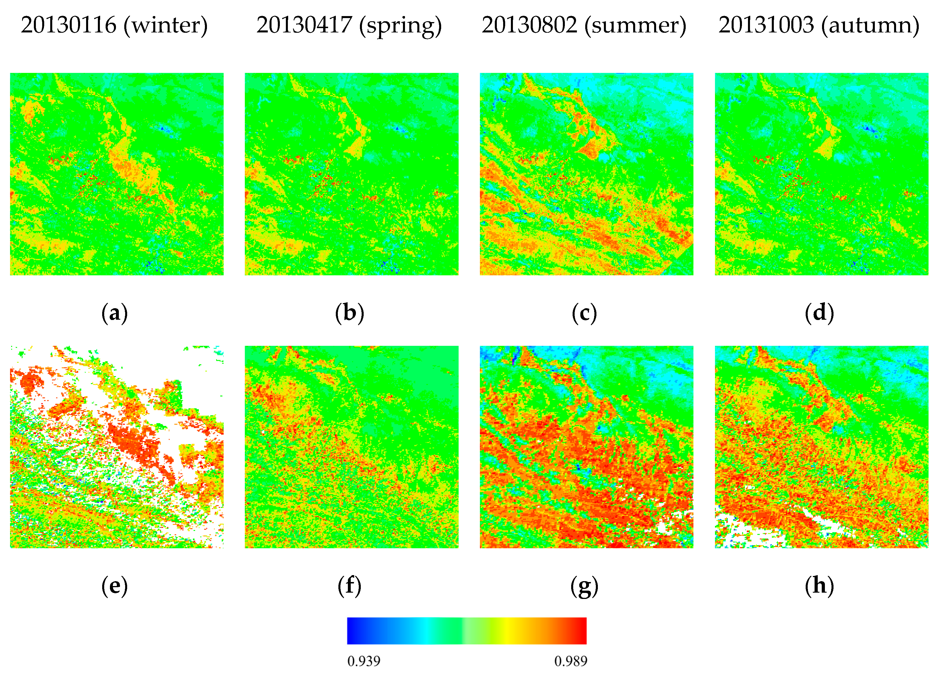
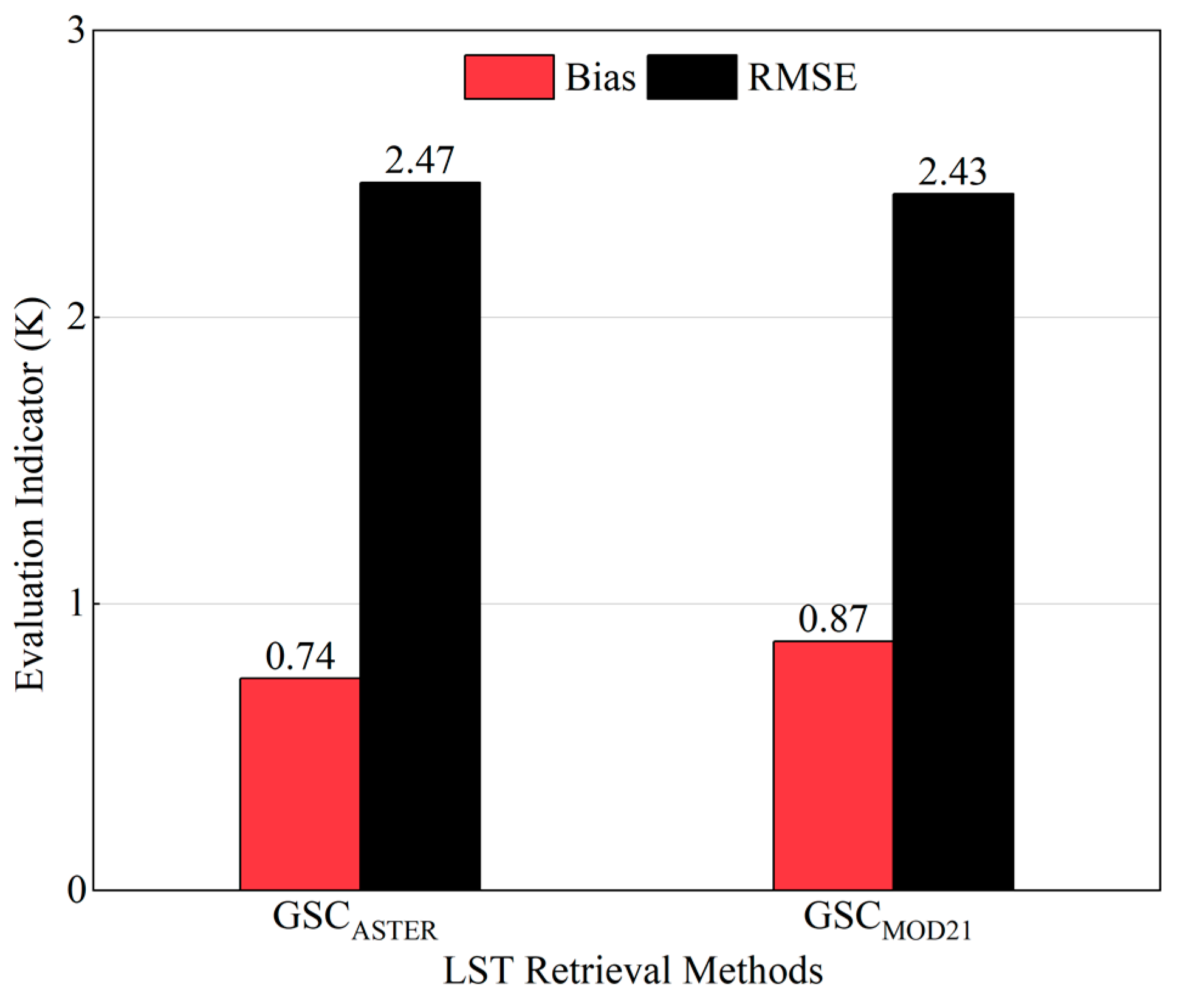
To improve the LSTs retrieved by the GSC algorithm, this study uses the ASTER GEDv3 product, and another physically retrieved emissivity product, MOD21, is generated by the TES algorithm, which can also support LST retrieval. This section aims to use the GSC algorithm to compare the effects of the two retrieved emissivity products. The emissivity of bands 31 and 32 of MOD21 was naturalized to band 4 of IRS, and the regression formula (17) is displayed below. Under the same atmospheric parameters, MOD21 was substituted into GSC to retrieve LST, which was marked as LSEMOD21. Figure 10 presents comparisons of the emissivity images for LSEASTER and LSEMOD21. Some variation exists among the products due to different sources and inconsistent spatial resolution. MOD21 has some missing values, but the high- and low-emissivity regions are the same as those from LSEASTER. Figure 11 displays the bias and RMSE of IRS LSTs calculated by LSEASTER and LSEMOD21. Compared with that of GSCMOD21, the bias of GSCASTER is reduced by 0.13 K, indicating that the accuracy of LSEASTER is slightly superior to that of LSEMOD21. Therefore, the physically retrieved emissivity products ASTER GEDv3 and MOD21 can support the LST retrieval of the GSC algorithm. ASTER GEDv3 provides static emissivity, whereas MOD10A1 provides dynamic emissivity that changes daily. MOD21 can directly provide dynamic emissivity that updates daily, and it has been used as support in retrieving LST for many remote sensing data [26,37].
, , and are the emissivity of band 4 of IRS and bands 31 and band 32 of MOD21, respectively.
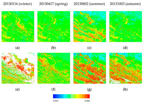
Figure 10.
Comparisons of the emissivity images for LSEASTER and LSEMOD21. (a–d) Emissivity images obtained by ASTER. (e–h) Emissivity images obtained by MOD21.
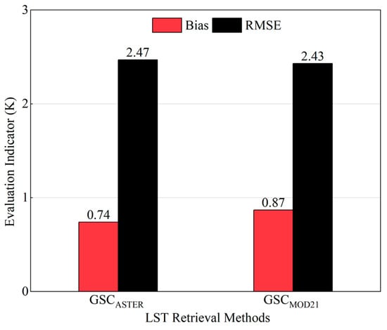
Figure 11.
Bias and RMSE of IRS LSTs calculated by LSEASTER and LSEMOD21.
6. Conclusions
Although HJ-1B/IRS has accumulated long-term observations, further application of IRS is considerably limited by the lack of LST products. Therefore, LST retrieval algorithms for HJ-1B/IRS data should be improved to generate HJ-1B/IRS LST products. To solve this problem, this study refined the ERA5 atmospheric profile database for the simulation of the coefficients of the GSCw and GSCwT algorithms. Then, we used the ASTER GEDv3 and vegetation/snow cover products using the VCM to calculate the LSE. Finally, the retrieved LSTs were evaluated using the LSTs from the RTE algorithm, TIGRw/TIGRwT profiles, and in situ near-surface air temperature. In general, we obtained the following conclusions from the validation results and discussion.
The bias (RMSE) values are displayed as ERA5wT < RTE < ERA5w < TIGRwT < TIGRw. The accuracy of LST obtained by GSCw/GSCwT from the refined ERA5 atmospheric profile database is higher than that obtained from the TIGR profiles. The accuracy of LST obtained by GSCwT is greater than that obtained by GSCw. The complex topography and large spatial heterogeneity of upstream sites lead to the overestimation of LST. The monthly changes indicate that the RMSEs are small during autumn and winter and large during spring and summer. In addition, the accuracy of LST retrieval decreases with an increase in WVC and VZA, and the GSC algorithm exhibits considerable accuracy in low WVC. The accuracy of LST obtained via in situ near-surface air temperature is higher than that obtained via ERA5 air temperature. The accuracy of LSEASTER is slightly better than that of LSEMOD21, and the physically retrieved ASTER GEDv3 and MOD21 can support the generation of HJ-1B/IRS LST products.
Based on the validation results, and considering the number of in situ near-surface air temperatures that can be applied to other regions, the ERA5wT that used WVC and ERA5 air temperature can improve the GSC algorithm for retrieving LST, and can generate long-term HJ-1B/IRS LST products. In the future, we will apply the algorithms to more regions and explore the benefits and shortcomings of LST retrieval algorithms on longer time series and under various atmospheric conditions.
Author Contributions
Conceptualization, D.L. and H.L.; methodology, H.L.; software, H.J.; validation, D.L., H.L. and G.Z.; formal analysis, G.Z.; investigation, Y.Y.; resources and data curation, Z.X., Z.H. and J.Z.; writing—original draft preparation, G.Z.; writing—review and editing, H.L.; visualization, G.Z.; supervision, D.L.; project administration, D.L.; funding acquisition, D.L., Z.X. and H.L. All authors have read and agreed to the published version of the manuscript.
Funding
This work was supported by the National Key R&D Program of China (2022YFB3903000, 2022YFB3903004) and the Chinese Natural Science Foundation Project (42071317).
Data Availability Statement
Not applicable.
Acknowledgments
We sincerely thank the China Centre for Resources Satellite Data and Application for providing free HJ-1B/IRS data, and the reviewers for their helpful comments.
Conflicts of Interest
The authors declare no conflict of interest.
References
- Li, Z.-L.; Tang, B.-H.; Wu, H.; Ren, H.; Yan, G.; Wan, Z.; Trigo, I.F.; Sobrino, J.A. Satellite-derived land surface temperature: Current status and perspectives. Remote Sens. Environ. 2013, 131, 14–37. [Google Scholar] [CrossRef]
- Lambin, E.F.; Ehrlich, D. Land-cover changes in sub-Saharan Africa (1982–1991): Application of a change index based on remotely sensed surface temperature and vegetation indices at a continental scale. Remote Sens. Environ. 1997, 61, 181–200. [Google Scholar] [CrossRef]
- Hansen, J.; Ruedy, R.; Sato, M.; Lo, K. Global Surface Temperature Change. Rev. Geophys. 2010, 48, RG4004. [Google Scholar] [CrossRef]
- Kogan, F.N. Operational space technology for global vegetation assessment. Bull. Am. Meteorol. Soc. 2001, 82, 1949–1964. [Google Scholar] [CrossRef]
- Hu, T.; van Dijk, A.I.J.M.; Renzullo, L.J.; Xu, Z.; He, J.; Tian, S.; Zhou, J.; Li, H. On agricultural drought monitoring in Australia using Himawari-8 geostationary thermal infrared observations. Int. J. Appl. Earth Obs. Geoinf. 2020, 91, 102153. [Google Scholar] [CrossRef]
- Wan, Z.; Dozier, J. A generalized split-window algorithm for retrieving land-surface temperature from space. IEEE Trans. Geosci. Remote Sens. 1996, 34, 892–905. [Google Scholar]
- Li, H.; Sun, D.; Yu, Y.; Wang, H.; Liu, Y.; Liu, Q.; Du, Y.; Wang, H.; Cao, B. Evaluation of the VIIRS and MODIS LST products in an arid area of Northwest China. Remote Sens. Environ. 2014, 142, 111–121. [Google Scholar] [CrossRef]
- Coll, C.; Caselles, V.; Valor, E.; Niclòs, R.; Sánchez, J.M.; Galve, J.M.; Mira, M. Temperature and emissivity separation from ASTER data for low spectral contrast surfaces. Remote Sens. Environ. 2007, 110, 162–175. [Google Scholar] [CrossRef]
- Du, C.; Ren, H.; Qin, Q.; Meng, J.; Zhao, S. A Practical Split-Window Algorithm for Estimating Land Surface Temperature from Landsat 8 Data. Remote Sens. 2015, 7, 647–665. [Google Scholar] [CrossRef]
- Qin, Z.; Karnieli, A.; Berliner, P. A mono-window algorithm for retrieving land surface temperature from Landsat TM data and its application to the Israel-Egypt border region. Int. J. Remote Sens. 2001, 22, 3719–3746. [Google Scholar] [CrossRef]
- Li, R.; Li, H.; Hu, T.; Bian, Z.; Liu, F.; Cao, B.; Du, Y.; Sun, L.; Liu, Q. Land Surface Temperature Retrieval from Sentinel-3A SLSTR data: Comparison among Split-window, Dual-window, Three-channel and Dual-angle algorithms. IEEE Trans. Geosci. Remote Sens. 2023, 61, 1–14. [Google Scholar] [CrossRef]
- Gillespie, A.; Rokugawa, S.; Matsunaga, T.; Cothern, J.S.; Hook, S.; Kahle, A.B. A temperature and emissivity separation algorithm for Advanced Spaceborne Thermal Emission and Reflection Radiometer (ASTER) images. IEEE Trans. Geosci. Remote Sens. 1998, 36, 1113–1126. [Google Scholar] [CrossRef]
- Li, H.; Liu, Q.; Du, Y.; Jiang, J.; Wang, H. Evaluation of the NCEP and MODIS Atmospheric Products for Single Channel Land Surface Temperature Retrieval With Ground Measurements: A Case Study of HJ-1B IRS Data. IEEE J. Sel. Top. Appl. Earth Obs. Remote Sens. 2013, 6, 1399–1408. [Google Scholar] [CrossRef]
- Duan, S.-B.; Li, Z.-L.; Wang, C.; Zhang, S.; Tang, B.-H.; Leng, P.; Gao, M.-F. Land-surface temperature retrieval from Landsat 8 single-channel thermal infrared data in combination with NCEP reanalysis data and ASTER GED product. Int. J. Remote Sens. 2018, 40, 1763–1778. [Google Scholar] [CrossRef]
- Windahl, E.; Beurs, K.d. An intercomparison of Landsat land surface temperature retrieval methods under variable atmospheric conditions using in situ skin temperature. Int. J. Appl. Earth Obs. Geoinf. 2016, 51, 11–27. [Google Scholar] [CrossRef]
- Jiménez-Muñoz, J.C.; Sobrino, J.A. A generalized single-channel method for retrieving land surface temperature from remote sensing data. J. Geophys. Res. 2003, 109, 8112. [Google Scholar] [CrossRef]
- Jimenez-Munoz, J.C.; Cristobal, J.; Sobrino, J.A.; Soria, G.; Ninyerola, M.; Pons, X.; Pons, X. Revision of the Single-Channel Algorithm for Land Surface Temperature Retrieval From Landsat Thermal-Infrared Data. IEEE Trans. Geosci. Remote Sens. 2009, 47, 339–349. [Google Scholar] [CrossRef]
- Pandya, M.R.; Shah, D.B.; Trivedi, H.J.; Darji, N.P.; Ramakrishnan, R.; Panigrahy, S.; Parihar, J.S.; Kirankumar, A. Retrieval of land surface temperature from the Kalpana-1 VHRR data using a single-channel algorithm and its validation over western India. Isprs J. Photogramm. Remote Sens. 2014, 94, 160–168. [Google Scholar] [CrossRef]
- Wang, X.; Zhong, L.; Ma, Y. Estimation of 30 m land surface temperatures over the entire Tibetan Plateau based on Landsat-7 ETM+ data and machine learning methods. Int. J. Digit. Earth 2022, 15, 1038–1055. [Google Scholar] [CrossRef]
- Sobrino, J.A.; Raissouni, N.; Li, Z.L. A Comparative Study of Land Surface Emissivity Retrieval from NOAA Data. Remote Sens. Environ. 2001, 75, 256–266. [Google Scholar] [CrossRef]
- Valor, E.; Caselles, V. Mapping land surface emissivity from NDVI: Application to European, African, and South American areas. Remote Sens. Environ. 1996, 57, 167–184. [Google Scholar] [CrossRef]
- Snyder, W.C.; Wan, Z.; Zhang, Y.; Feng, Y.Z. Classification-based emissivity for land surface temperature measurement from space. Int. J. Remote Sens. 1998, 19, 2753–2774. [Google Scholar] [CrossRef]
- Duan, S.-B.; Li, Z.-L.; Li, H.; Göttsche, F.-M.; Wu, H.; Zhao, W.; Leng, P.; Zhang, X.; Coll, C. Validation of Collection 6 MODIS land surface temperature product using in situ measurements. Remote Sens. Environ. 2019, 225, 16–29. [Google Scholar] [CrossRef]
- Hulley, G.C.; Hook, S.J.; Abbott, E.; Malakar, N.; Islam, T.; Abrams, M. The ASTER Global Emissivity Dataset (ASTER GED): Mapping Earth’s emissivity at 100 meter spatial scale. Geophys. Res. Lett. 2015, 42, 7966–7976. [Google Scholar] [CrossRef]
- Li, H.; Hu, T.; Meng, X.; Du, Y.; Cao, B.; Liu, Q. Improving HJ-1B IRS land surface temperature product using ASTER global emissivity dataset. In Proceedings of the 2016 IEEE International Geoscience and Remote Sensing Symposium (IGARSS), Beijing, China, 10–15 July 2016; 2016; pp. 2661–2664. [Google Scholar]
- Li, H.; Yang, Y.K.; Li, R.B.; Wang, H.S.; Cao, B.; Bian, Z.J.; Hu, T.; Du, Y.M.; Sun, L.; Liu, Q.H. Comparison of the MuSyQ and MODIS Collection 6 Land Surface Temperature Products Over Barren Surfaces in the Heihe River Basin, China. IEEE Trans. Geosci. Remote Sens. 2019, 57, 8081–8094. [Google Scholar] [CrossRef]
- Zhang, S.; Duan, S.-B.; Li, Z.-L.; Huang, C.; Wu, H.; Han, X.-J.; Leng, P.; Gao, M. Improvement of Split-Window Algorithm for Land Surface Temperature Retrieval from Sentinel-3A SLSTR Data Over Barren Surfaces Using ASTER GED Product. Remote Sens. 2019, 11, 3025. [Google Scholar] [CrossRef]
- Wang, H.; Yu, Y.; Yu, P.; Liu, Y. Land Surface Emissivity Product for NOAA JPSS and GOES-R Missions: Methodology and Evaluation. IEEE Trans. Geosci. Remote Sens. 2020, 58, 307–318. [Google Scholar] [CrossRef]
- Li, R.; Li, H.; Sun, L.; Yang, Y.; Hu, T.; Bian, Z.; Cao, B.; Du, Y.; Liu, Q. An Operational Split-Window Algorithm for Retrieving Land Surface Temperature from Geostationary Satellite Data: A Case Study on Himawari-8 AHI Data. Remote Sens. 2020, 12, 2613. [Google Scholar] [CrossRef]
- Abrams, M.; Crippen, R.; Fujisada, H. ASTER Global Digital Elevation Model (GDEM) and ASTER Global Water Body Dataset (ASTWBD). Remote Sens. 2020, 12, 1156. [Google Scholar] [CrossRef]
- Zhao, J.; Li, J.; Liu, Q.; Xu, B.; Yu, W.; Lin, S.; Hu, Z. Estimating fractional vegetation cover from leaf area index and clumping index based on the gap probability theory. Int. J. Appl. Earth Obs. Geoinf. 2020, 90, 102112. [Google Scholar] [CrossRef]
- Hersbach, H.; Bell, B.; Berrisford, P.; Hirahara, S.; Horányi, A.; Muñoz-Sabater, J.; Nicolas, J.; Peubey, C.; Radu, R.; Schepers, D. The ERA5 global reanalysis. Q. J. R. Meteorol. Soc. 2020, 146, 1999–2049. [Google Scholar] [CrossRef]
- Muñoz-Sabater, J.; Dutra, E.; Agustí-Panareda, A.; Albergel, C.; Arduini, G.; Balsamo, G.; Boussetta, S.; Choulga, M.; Harrigan, S.; Hersbach, H. ERA5-Land: A state-of-the-art global reanalysis dataset for land applications. Earth Syst. Sci. Data 2021, 13, 4349–4383. [Google Scholar] [CrossRef]
- Cristóbal, J.; Jiménez-Muñoz, J.C.; Sobrino, J.A.; Ninyerola, M.; Pons, X. Improvements in land surface temperature retrieval from the Landsat series thermal band using water vapor and air temperature. J. Geophys. Res. Atmos. 2009, 114, D08103. [Google Scholar] [CrossRef]
- Li, X.; Cheng, G.; Liu, S.; Xiao, Q.; Ma, M.; Jin, R.; Che, T.; Liu, Q.; Wang, W.; Qi, Y.; et al. Heihe Watershed Allied Telemetry Experimental Research (HiWATER): Scientific Objectives and Experimental Design. Bull. Am. Meteorol. Soc. 2013, 94, 1145–1160. [Google Scholar] [CrossRef]
- Liu, S.; Li, X.; Xu, Z.; Che, T.; Xiao, Q.; Ma, M.; Liu, Q.; Jin, R.; Guo, J.; Wang, L.; et al. The Heihe Integrated Observatory Network: A Basin-Scale Land Surface Processes Observatory in China. Vadose Zone J. 2018, 17, 1–21. [Google Scholar] [CrossRef]
- Li, H.; Li, R.; Yang, Y.; Cao, B.; Liu, Q. Temperature-Based and Radiance-Based Validation of the Collection 6 MYD11 and MYD21 Land Surface Temperature Products Over Barren Surfaces in Northwestern China. IEEE Trans. Geosci. Remote Sens. 2021, 59, 1794–1807. [Google Scholar] [CrossRef]
- Li, H.; Li, R.; Tu, H.; Cao, B.; Liu, F.; Bian, Z.; Hu, T.; Du, Y.; Sun, L.; Liu, Q. An Operational Split-Window Algorithm for Generating Long-Term Land Surface Temperature Products from Chinese Fengyun-3 Series Satellite Data. IEEE Trans. Geosci. Remote Sens. 2023. [Google Scholar] [CrossRef]
- Ermida, S.L.; Trigo, I.F. A Comprehensive Clear-Sky Database for the Development of Land Surface Temperature Algorithms. Remote Sens. 2022, 14, 2329. [Google Scholar] [CrossRef]
- Peres, L.F.; DaCamara, C.C. Emissivity maps to retrieve land-surface temperature from MSG/SEVIRI. IEEE Trans. Geosci. Remote Sens. 2005, 43, 1834–1844. [Google Scholar] [CrossRef]
- Baldridge, A.M.; Hook, S.J.; Grove, C.I.; Rivera, G. The ASTER spectral library version 2.0. Remote Sens. Environ. 2009, 113, 711–715. [Google Scholar] [CrossRef]
- Coll, C.; Caselles, V.; Galve, J.; Valor, E.; Niclos, R.; Sanchez, J.; Rivas, R. Ground measurements for the validation of land surface temperatures derived from AATSR and MODIS data. Remote Sens. Environ. 2005, 97, 288–300. [Google Scholar] [CrossRef]
Disclaimer/Publisher’s Note: The statements, opinions and data contained in all publications are solely those of the individual author(s) and contributor(s) and not of MDPI and/or the editor(s). MDPI and/or the editor(s) disclaim responsibility for any injury to people or property resulting from any ideas, methods, instructions or products referred to in the content. |
© 2023 by the authors. Licensee MDPI, Basel, Switzerland. This article is an open access article distributed under the terms and conditions of the Creative Commons Attribution (CC BY) license (https://creativecommons.org/licenses/by/4.0/).