Communication

Long-Term Observations of the Thermospheric 6 h Oscillation Revealed by an Incoherent Scatter Radar over Arecibo

1
Electronic Information School, Wuhan University, Wuhan 430072, China
2
Guizhou Normal University, Guiyang 550025, China
3
Electrical and Computer Engineering Department, Miami University, Oxford, OH 45056, USA
*
Author to whom correspondence should be addressed.
Remote Sens. 2023, 15(21), 5098; https://doi.org/10.3390/rs15215098
Submission received: 12 September 2023 / Revised: 13 October 2023 / Accepted: 24 October 2023 / Published: 25 October 2023
(This article belongs to the Special Issue Atmospheric Dynamics with Radar Observations)

Abstract

:
We present an analysis of 6 h oscillations in the thermosphere ranging from 150 km to 400 km. The analysis applies 134 days of data from an incoherent scatter radar located at Arecibo Observatory (18.3°N, 66.7°W) from 1984 to 2015. To our knowledge, the climatological and seasonal characteristics of the 6 h oscillations in the thermosphere were investigated for the first time over Arecibo. The climatological mean amplitude of the 6 h oscillation in the thermosphere is about 11 m/s, and it increases slowly with altitude above 225 km. The climatological mean amplitude of the 6 h oscillation is comparable with semidiurnal and terdiurnal tides at Arecibo above 250 km. The climatological mean phase exhibits limited vertical variation. The 6 h oscillation is the most prominent in autumn, with amplitudes reaching around 20 m/s compared to approximately 10 m/s in other seasons. The phase structure in all seasons exhibits weak vertical variations. The responses of the thermospheric 6 h oscillation to solar and geomagnetic activities are also analyzed in this study. Our results indicate that at low latitude, solar activities have a small impact on the variation in the thermospheric 6 h oscillation, while it appears that the amplitude of the 6 h oscillation increases with increasing geomagnetic activity. Above 250 km, the amplitude of the 6 h oscillation reaches ~20 m/s during strong geomagnetic activity, which is almost twice of that occurring during weak geomagnetic activity.

1. Introduction

Atmospheric solar tides are large-scale oscillations that play an important role in the dynamics of the atmosphere and ionosphere. The solar tides are mainly generated by solar heating, and therefore their periods are related to a solar day. Tidal waves with periods of 24 h, 12 h, 8 h, and 6 h are generally recognized as diurnal (DT), semidiurnal (SDT), terdiurnal (TDT), and 6 h tides, respectively. With the increase in satellite and ground-based measurements, our understanding of the tidal waves in the atmosphere has significantly increased in recent decades [1,2,3,4,5,6,7,8,9,10,11,12,13,14,15,16]. However, the majority of previous studies focus on investigating the characteristics of diurnal, semidiurnal, and terdiurnal tides because of their large amplitudes and can be frequently observed. The transient behavior and small amplitudes of 6 h tides make them difficult to observe, and their characteristics are not well understood.
In the mesosphere and lower thermosphere (MLT) region, several studies have reported the characteristics of 6 h tides using meteor radars [17,18,19,20,21], medium-frequency (MF) radars [22,23], lidar temperature observation [24], airglows [25,26], satellite observations [27,28,29,30,31], and numerical models [32,33]. Using meteor radar measurements at Collm (51°N, 13°E) and Obninsk (55°N, 37°E), Jacobi et al. [17] investigated seasonal variations in 6 h tides in the MLT region. Their results indicated that the maximum amplitudes of 6 h tides occur in winter, and zonal amplitudes are greater than meridional ones on average. Jacobi et al. [18] studied the forcing mechanism of the 6 h tides, and they found that self-interaction of SDTs is important in generating the 6 h tide winter. Pancheva et al. [20] reported seasonal and altitudinal variations in 6 h tides at high latitudes using the Tromsø (70°N, 19°E) and Svalbard (78°N, 16°E) meteor radars. Their results indicated that 6 h tides have a maximum amplitude in winter and a minimum amplitude in summer. Using 9 years of observation data from a meter radar located at Mohe (53.5°N, 122.3°E), Gong et al. [11] found that the amplitude of the 6 h tide was very strong, reaching ~10 m/s during the 2019 sudden stratospheric warming. They concluded that the strong amplitude of the 6 h tide is due to the nonlinear interaction between two SDTs. Using three meteor radars located at low latitudes in the Southern Hemisphere, Guharay et al. [19] concluded that the amplitude of 6 h tides is much smaller than that of tidal components with longer periods for most of the year, and the seasonal variation in 6 h tides is not prominent. Based on neural wind data obtained from a meteor radar at South Georgia (54°S, 36°W), Hindley et al. [21] found that the amplitude of 6 h tides is weaker than that of the other tidal components with longer periods. Using data obtained from MF radar stations at Adelaide (35°S, 138°E) and Davis (68°S, 78°E), Kovalam et al. [22] found the highest activity of 6 h oscillations occurs in solstitial months, especially winter. Liu et al. [23] reported a 6 h tidal signature in MF radar data over Wuhan and suggested that nonlinear interactions are likely a generation mechanism of the 6 h tide. Based on satellite temperature measurements, Xu et al. [28] suggested that nonlinear interactions between diurnal and terdiurnal tides are an important mechanism in exciting the 6 h tide. Liu et al. [29] studied the global structure and seasonal variations in 6 h tides. Their study indicated that although the 6 h tide is weaker than that of the diurnal and semirural tides, it is a persistent feature in the lower thermosphere. Using satellite observations, Azeem et al. [30] observed that the magnitude of the 6 h tide increases from ~5 K to ~30 K from about 100 km to 130 km, which indicates that the 6 h tide is important in the lower thermosphere. Based on a nonlinear global circulation model, Geißler et al. [33] suggested that tide–tide interactions, gravity wave–tide interactions, and the absorption of solar radiation are the possible generation mechanisms of the 6 h tide.
Due to the limitations of detecting techniques, few studies have investigated the characteristics of 6 h tides above 120 km. Tong et al. [34] found 6 h tides in the upper E region (above 110 km) based on Arecibo (18.3°N, 66.7°W) incoherent scatter radar (ISR) measurements in the period of 3–6 January 1981. Using the Arecibo ISR measurements from 5 to 10 February 2016, Gong et al. [35] found a strong 6 h tide in the thermosphere at low latitude. Above 280 km, the observed 6 h tidal amplitude was about 1.5 times larger than the amplitude of the semidiurnal tide. Their results indicate that the 6 h oscillation could be a major contributor to the thermospheric dynamics. Gong et al. [35] suggested that nonlinear interactions between diurnal and terdiurnal tides are important in generating the observed 6 h tide. However, to our knowledge, the climatology and seasonal variations in the 6 h oscillation in the thermosphere have not been reported.
In this study, we investigate the climatology and seasonal variations in the thermospheric 6 h oscillation at low latitude using observation data obtained from the Arecibo ISR from 1984 to 2015. The responses of the 6 h oscillation to solar and geomagnetic activities are also investigated. Section 2 describes the radar observations and data processing methods used in this study. Section 3 presents the results of climatological and seasonal characteristics of 6 h oscillations and the variations in the thermospheric 6 h tide under different solar and geomagnetic activities. Discussions and conclusions are presented in Section 4 and Section 5, respectively.

2. Data Analysis

Gordon [36] demonstrated that electrons in the ionosphere can scatter a sufficient amount of energy to be detected by a realistically powerful radar. In 1960, Gordon led the construction of the world’s largest ISR near Arecibo, Puerto Rico, a karst region with sinkholes suitable for building large dish antennae. The reflective parabolic antenna of the Arecibo ISR has a diameter of 305 m, and the antenna’s effective gain is 41.7 DB/m2. The radar has a peak power of 2.5 MW and operates at 430 MHz. The Arecibo ISR has the advantage of high transmitting power and a high signal-to-noise ratio, and it provided continuous detection information from its establishment in 1963 to its collapse on 1 December 2020. Among the 40 days of radar operation per year, 20 days were devoted to the “world-day”, a common mode run by most of the incoherent scatter radars in the world. Although all world-day data should be archived in the database, the actual number of data archived depended on a variety of factors, including system conditions and staff priorities.
In this study, 134 days of data collected from the Arecibo ISR measurements from 1984 to 2015 were used, which is all the “world-day” data that we can find in the database. A multiple radar autocorrelation function (MRACF) method that measures several ionosphere parameters from ~150 to ~680 km was used to obtain the power spectrum [37]. The corresponding temporal and altitudinal resolutions were ~90 s and ~38 km, respectively [37]. The MRACF technique phase-coded the transmitter pulse in such a way that seven frequencies were transmitted simultaneously. Although the power in each frequency is reduced, this resulted in a 7-fold increase in independent samples and a significantly higher overall signal-to-noise ratio. This technique is discussed by Sulzer [37], and application examples can be found in Isham et al. [38]. A linear regularized inversion method was applied in this study to convert the line-of-sight velocities to vector velocities [39]. The 134 days of data were divided into 80 segments. Each segment had 18 consecutive hours of data, which means that each segment has three cycles of data when fitting the 6 h oscillations. In order to investigate the variations in 6 h oscillations under different seasons and solar and geomagnetic activities, the following definitions were made in this study. The four seasons are defined as spring (March, April, May), summer (June, July, August), autumn (September, October, November), and winter (December, January, February). We define the F10.7 ≥ 140 solar flux unit (SFU = 10–22 W/m2/Hz), 100 SFU ≤ F10.7 < 140 SFU, and F10.7 < 100 SFU as high, moderate, and low solar activities, respectively, and KP ≥ 4, 2 ≤ KP < 4, and KP < 2 as strong, moderate, and weak geomagnetic activities, respectively. Cai et al. [40] stated that the impact of geomagnetic forcing can last more than 1 day. Thus, we not only examined the geomagnetic conditions on the day with available data but also considered the conditions on the previous two days. Figure 1 presents the number of segments in each category. As shown in Figure 1a, there are 19 segments in spring, 18 segments in summer, 22 segments in autumn, and 21 segments in winter. As seen from Figure 1b,c, the statistics under high, moderate, and low solar activities consist of 17 segments, 26 segments, and 37 segments, and strong, moderate, and weak geomagnetic activities consist of 12 segments, 44 segments, and 24 segments, respectively.
Using the ISR measurements, meridional winds in the thermosphere can be deduced via [41]
u = v / / v d s e c I
where u represents the meridional wind, I denotes the dip angle, v / /   is the ion drift velocity with a direction antiparallel to the geomagnetic field, and v d represents the diffusion velocity. v d can be obtained from the following formula [42]:
v d = D T 1 T 2 sin I d ln n e d z + 1 H + d ln T 1 d z + 0.36 d ln T 2 d z
where n e is the electron density, z represents the altitude, H = 2 k T 1 m i g , and D denotes the ambipolar diffusion coefficient, as follows:
D = 2 k T i m i v i n
where T i represents the ion temperature, k denotes the Boltzmann constant, and m i is the ion mass. In the F-region, the major ion species is represented by O + . The ion-neutral collision frequency ( v i n ) of O + with neutral particles can be obtained from the formula below [42]:
v i n = k 0.3 T 2 0.5 1 0.135 log T 2 1000 2 + 6.7 O + 6.9 O 2 + 6.9 N 2 519.6 × 10 16 m O +
where T 1 = T i + T e 2 , T 2 = T i + T n 2 , T e is the electron temperature, T n is the neutral temperature, and m O + denotes the mass of O + in atomic mass units. O , O 2 , and N 2 are densities of the neutral particles, and their unit is cm−3. Neutral parameters were obtained from the MSIS-E-00 atmosphere model. The deduced meridional wind from 17 to 20 November 2005 over Arecibo is presented in Figure 2. The white areas are data gaps due to low electron density in the nighttime. Note that the obtained meridional wind using the Arecibo ISR has a measurement error of 10 m/s [35]. Since the ambipolar coefficient above 400 km has large uncertainties [43], this study only presents the derived meridional wind below 400 km.
After obtaining the thermospheric meridional wind, a high-pass filter with a cutoff frequency of 7 h was applied to suppress the effect of interference components such as diurnal and semidiurnal tides on the fitting results of the 6 h oscillations. Then, the least-squares fitting method was applied to extract the amplitudes and phases of the 6 h oscillation in each segment from the filtered meridional wind ( u t ) using the following formula:
u t = A 0 + A 1 cos 2 π 24 × t + B 1 sin 2 π 24 × t + A 2 cos 2 π 12 × t + B 2 sin 2 π 12 × t + A 3 cos 2 π 8 × t + B 3 sin 2 π 8 × t + A 4 cos 2 π 6 × t + B 4 sin 2 π 6 × t
where A 0 is the mean meridional wind and A 4 and B 4 are the magnitudes of the 6 h oscillation. The amplitude (Amp) and phase (Ph) of the 6 h oscillation can be obtained using the following equation:
A m p = A 4 2 + B 4 2   ( m / s )
P h = 3 arctan B 4 A 4 π   ( h )

3. Results

3.1. Climatological Characteristics

The fitting results in each segment were averaged together to investigate the climatological characteristics of the thermospheric 6 h oscillation. The climatological amplitude (red) and phase (blue) results are shown in Figure 3. As shown in Figure 3, the climatological mean amplitude of the 6 h oscillation was about 11 m/s. Above 225 km, the amplitude increased slowly with altitude and the amplitude reached the maximum of ~14 m/s at about 380 km. In order to reveal the variability in the climatological mean amplitude, the standard deviations of the climatological average were calculated and are represented by the error bars shown in Figure 3. Based on our results, the standard deviations varied in a range of 50–60% of the climatological mean amplitude. The phase of the 6 h oscillation was essentially constant and varied slightly around 0:00 LT. Gong et al. [43] reported the climatological characteristics of the thermospheric DT, SDT, and TDT using the Arecibo ISR measurements. They found that above 250 km, the climatological mean amplitudes of the DT, SDT, and TDT are approximately 20 m/s, 15 m/s, and 15 m/s, respectively. The SDT amplitude in the height range 150 to 250 km is the strongest, and its maximum is about 33 m/s. Below 250 km, the DT and TDT amplitudes vary at about 25 m/s and 15 m/s, respectively. Our analysis revealed that the climatological mean amplitude of the 6 h oscillation in the thermosphere was much smaller than that of other tidal components with longer periods. Gong et al. [43] also calculated the variabilities in the climatological mean amplitudes of the three tidal components. The standard deviations of the DT, SDT, and TDT fall in intervals of 50–70%, 50–60%, and 30–50% of the mean amplitudes of the DT, SDT, and TDT, respectively. Our results indicate that the variability in the 6 h oscillation was not much different to that of the DT and SDT but was greater than that of the TDT. Above 250 km, the climatological mean phase structure of the 6 h oscillation was largely consistent with the other three tidal components. Below 250 km, the phases of the SDT and TDT exhibited a clear downward progression [43]. The phase structure of the 6 h oscillation indicates that direct solar heating is very important in generating the thermospheric 6 h oscillation.

3.2. Seasonal Characteristics

Figure 4 presents the vertical variations in the 6 h oscillation amplitudes (red) and phases (blue) in spring, summer, autumn, and winter, respectively. As in the analysis of the climatological characteristics, the standard deviations of mean amplitudes and phases were computed to reveal the variabilities in the 6 h oscillations during different seasons, which are indicated by the error bars. As shown in the first column of Figure 4, the mean amplitude of the 6 h oscillation was about 10 m/s in spring. The standard deviations varied in a range of 45–55% of the mean amplitude above 180 km. In spring, the mean phase of the 6 h oscillation had weak vertical variations. In summer, the average amplitude of the 6 h oscillation was about 10 m/s, as in spring. The standard deviations fell in an interval of 40–65% of the mean amplitude. According to the first and second columns of Figure 4, above 250 km, the amplitude variation in the 6 h oscillation in summer was greater than in spring. The mean phase of the 6 h oscillation in summer had limited vertical variation above 180 km.
In autumn, the mean amplitude of the 6 h oscillation was much stronger than in spring and summer. The mean amplitude of the 6 h oscillation in autumn was about 15 m/s, and the amplitude increased with height from 10 m/s at 150 km to 20 m/s at 380 km. The standard deviations varied in a range of 40–65% of the mean amplitude, which is the same as that in summer. The mean phase of the 6 h oscillation varied around 0:00 LT with limited vertical variation. It appears that the vertical structure of the mean phase in autumn had almost the same trend as the climatological mean phase structure. In winter, the average amplitude of the 6 h oscillation was about 10 m/s. The mean amplitude of the 6 h oscillation first decreased with height, reaching a minimum of 8 m/s at 225 km, and then increased with height, arriving at a peak value of 14 m/s at 380 km. The standard deviations fell in an interval of 30–50% of the mean amplitude, which indicates that the variability in winter is the smallest among the four seasons. The vertical structure of the mean phase of the 6 h oscillation in winter was consistent with that in autumn.
Our results reveal that the thermospheric 6 h oscillations at low latitude had the strongest amplitude in autumn and exhibited a clear pattern of amplitude increasing with height. The mean amplitude at the other three seasons was comparable. Gong et al. [43] reported that above 180 km, the DT, SDT, and TDT are the most prominent in winter, autumn, and winter, respectively. It appears that the 6 h oscillation and the SDT both had the strongest amplitude in autumn. Above 200 km, the phase structures in the four seasons were largely consistent, and the vertical variation was limited.

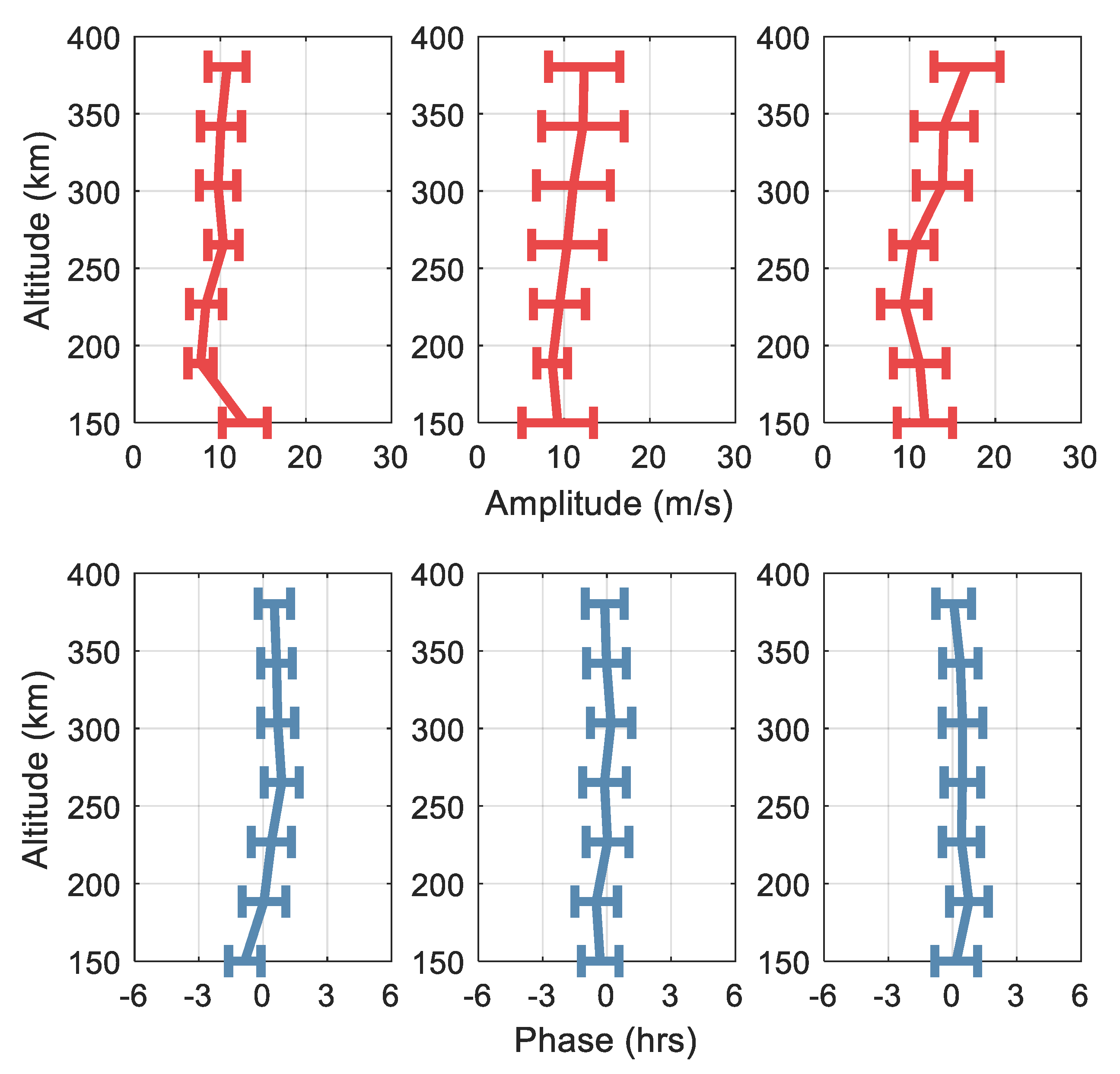
3.3. Characteristics under Different Solar Activities

Figure 5 presents the amplitudes (first row) and phases (second row) of the thermospheric 6 h oscillations under high, moderate, and low solar activities, respectively. The standard deviations of the mean amplitudes and phases during different solar activities were also calculated. As seen from Figure 5, the average amplitude of the 6 h oscillation was 10 m/s under high solar activity. Above 180 km, the average amplitude of the 6 h oscillation varied slightly around 10 m/s. The standard deviations were about 35–45% of the mean amplitude. Under moderate solar activity, above 180 km, the amplitude of the 6 h oscillation increased slowly with altitude. The average amplitude was 10 m/s, and the peak amplitude was 12 m/s. The standard deviations varied in a range of 40–80% of the average amplitude, which indicates that the variability in the moderate solar activity was much larger than under the high solar activity. During low solar activity, the amplitude of the 6 h oscillation fluctuated around 10 m/s below 250 km. Above that height, the amplitude of the 6 h oscillation increased with altitude. The mean amplitude during low solar activity was 12 m/s. The standard deviations were about 45–60% of the mean amplitude. The altitudinal variation in the mean phases of the 6 h oscillations was largely consistent under different solar activities, and it had limited vertical variation. According to our results, the average amplitudes were 10 m/s, 10 m/s, and 12 m/s under high, medium, and low solar activities, respectively. The amplitudes of the 6 h oscillation had a small increase during the low solar activity. The results indicate that the response of the 6 h oscillation to solar activities was not significant. Using data collected from the Arecibo ISR, Gong et al. [43] reported that the amplitude of the DT increased while the SDT amplitude was reduced with an increase in solar activity. They reported that the variation in the TDT is not sensitive to solar activities. Our conclusion for 6 h oscillations is consistent with the results found for TDT by [43]. It may be possible that solar activities have a weak influence on oscillations with short periods.

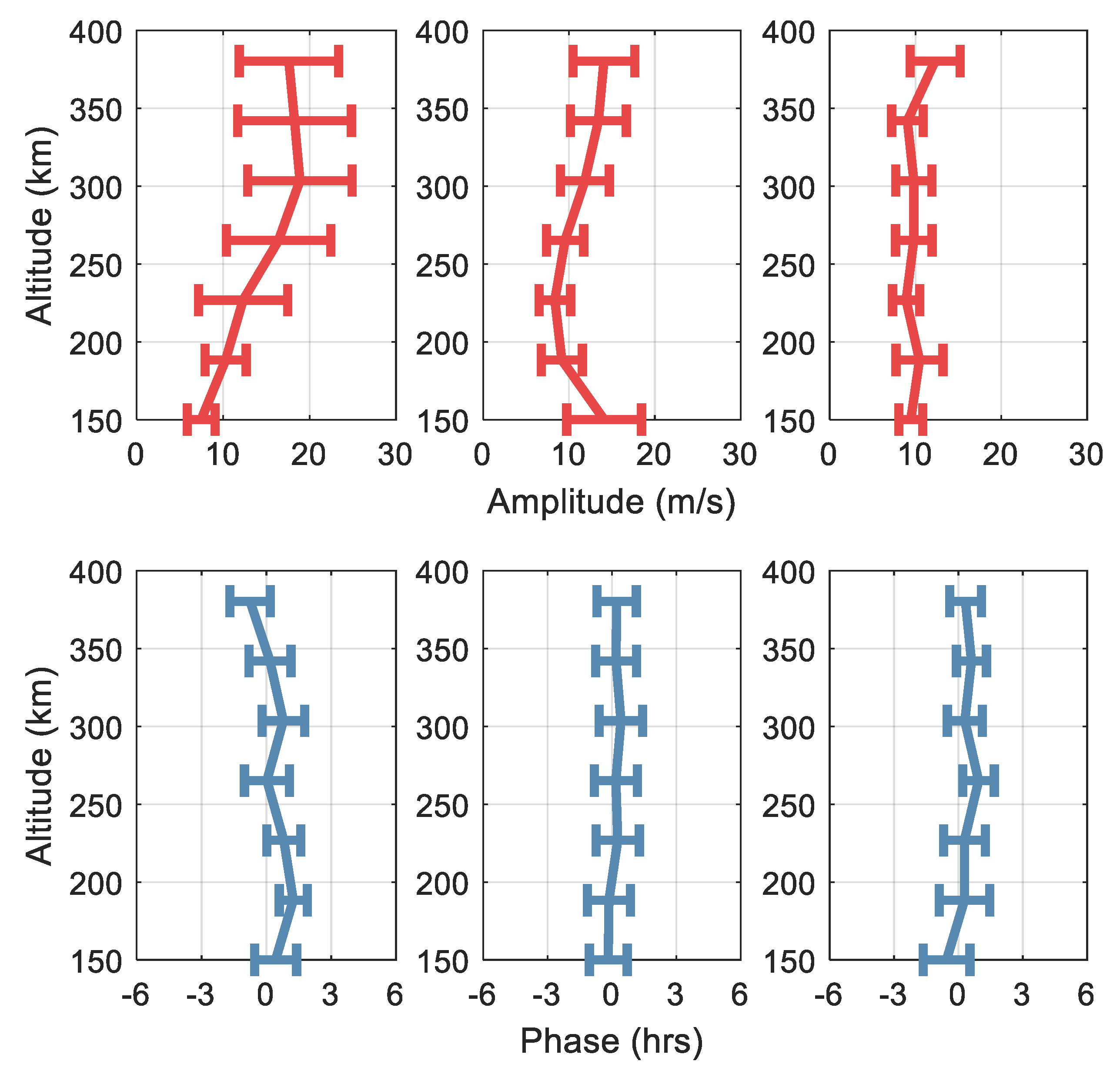
3.4. Characteristics under Different Geomagnetic Activities

The amplitudes (first row) and phases (second row) of the 6 h oscillation under strong, moderate, and weak geomagnetic activities in the thermosphere are presented in Figure 6. The standard deviations during different geomagnetic activities were also obtained. As shown in Figure 6, during strong geomagnetic activity, the averaged amplitude of the 6 h oscillation was approximately 14 m/s. The amplitude increased rapidly at altitudes below 250 km. Above 250 km, the mean amplitude had limited vertical variations, and it varied around 18 m/s. The standard deviations were about 40–85% of the mean amplitude. During moderate geomagnetic activity, the amplitude of the 6 h oscillation first decreased and then increased with altitude, and the average amplitude was 12 m/s. The standard deviations varied within an interval of 45–60% of the average amplitude. During weak geomagnetic activity, the amplitude of the 6 h oscillation had a small vertical variation and the mean amplitude was 10 m/s. The standard deviations were about 30–55% of the average amplitude during weak geomagnetic activity, which was the smallest value found among different geomagnetic activities. According to our results, the highest average amplitude of the 6 h oscillation occurred during strong geomagnetic activity, and the amplitude of the 6 h oscillations under moderate geomagnetic activity was slightly larger than the amplitude under low geomagnetic activity. Above 250 km, the amplitude of the 6 h oscillation during strong geomagnetic activity was about two times larger than that occurring during weak geomagnetic activity. The vertical phase structure of the 6 h oscillation was largely consistent during different geomagnetic activities. A small difference is that the vertical variation during strong geomagnetic activity was larger than that occurring during moderate and weak geomagnetic activity. Our results indicate that the amplitude of the 6 h oscillation tends to increase with the intensification of geomagnetic activities above 200 km. Note that, as shown in Figure 1b, although the category of strong geomagnetic activity included 12 samples, this number is still much smaller than the number of segments in the other two categories. Hence, our results may have a bias due to uneven sample sizes.

4. Discussion

Aside from atmospheric tides, gravity waves can also have a period of 6 h. The difference between tidal waves and gravity waves is that the former has a coherent phase while the phase of gravity waves is irregular. Using the Arecibo ISR data from 17 to 20 November 2005, we calculated the temporal phase variation in the 6 h oscillation at 300 km, and the result is shown in Figure 7a. We first passed the meridional wind data through a high-pass filter with a cutoff period of 7 h. Then, an 18 h sliding window with a step of 6 h was used, and the least-squares fitting method was applied in each window. As we can see from Figure 7a, the phase of the 6 h oscillation was locked, having weak temporal variations. This indicates that the observed 6 h oscillation was a tidal wave. To further investigate the evolution of the 6 h oscillation phases, a superposed epoch analysis [12,32] was used. After passing the meridional wind data through the high-pass filter, we composited the filtered data into one day, and the result is presented in Figure 7b. The structure of four crests and four troughs is exhibited in Figure 7b, which indicates that the phase of the 6 h oscillation was regular. This further verifies that the observed 6 h oscillation was a tidal wave. For a data duration of less than 2 days, it is hard to determine its phase structure. However, this study focused on analyzing the climatological and seasonal characteristics of the 6 h oscillation and the responses of the 6 h oscillation to solar and geomagnetic activities. Averaging a large number of fitted results may reduce the effect of gravity waves. Note that as this study was based on data collected from a single location, the spatial variation in the 6 h oscillation cannot be revealed. It is possible that other large-scale structures contributed to the vertical variation in the reported 6 h oscillation. We reasonably speculate that the statistical results shown in Section 3 are largely due to the effect of 6 h tides.

5. Conclusions

Previous studies reported that the 6 h oscillation could be an important dynamic process in the thermosphere at low latitudes. However, to our knowledge, the long-term variations in the 6 h oscillations in the height range 150 to 400 km at low latitude have not previously been reported. In this study, using 134 days of data measured using the incoherent scatter radar at Arecibo Observatory from 1984 to 2015, the climatological and seasonal characteristics of the 6 h oscillations and the variations in 6 h oscillations during different solar and geomagnetic activities were investigated. The altitudinal variation in the thermospheric 6 h oscillation at a low latitude was revealed. The major findings of this work are summarized as follows:
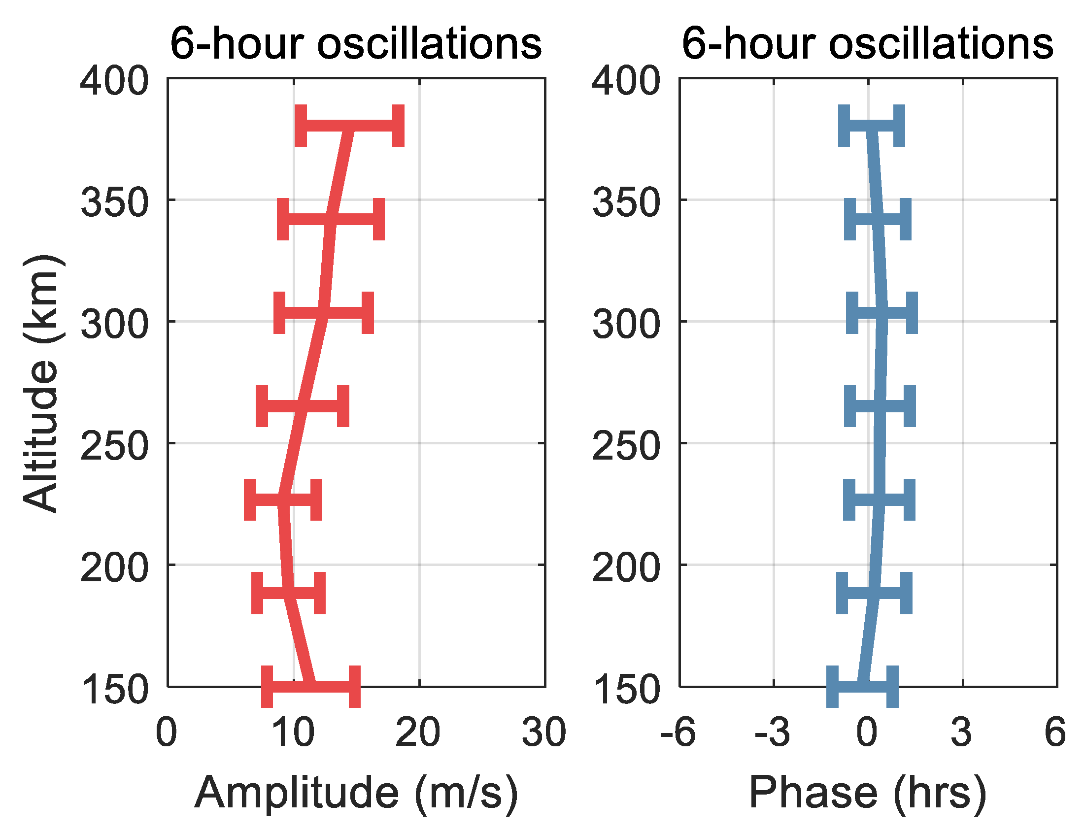
  • The climatological mean amplitude of the 6 h oscillation is about 11 m/s, and it increases slowly with increasing altitude above 225 km. The climatological mean 6 h oscillation is much smaller than the diurnal tide while being comparable with the semidiurnal and terdiurnal tides above 250 km. The climatological mean phase of the 6 h oscillation exhibits limited vertical variation.
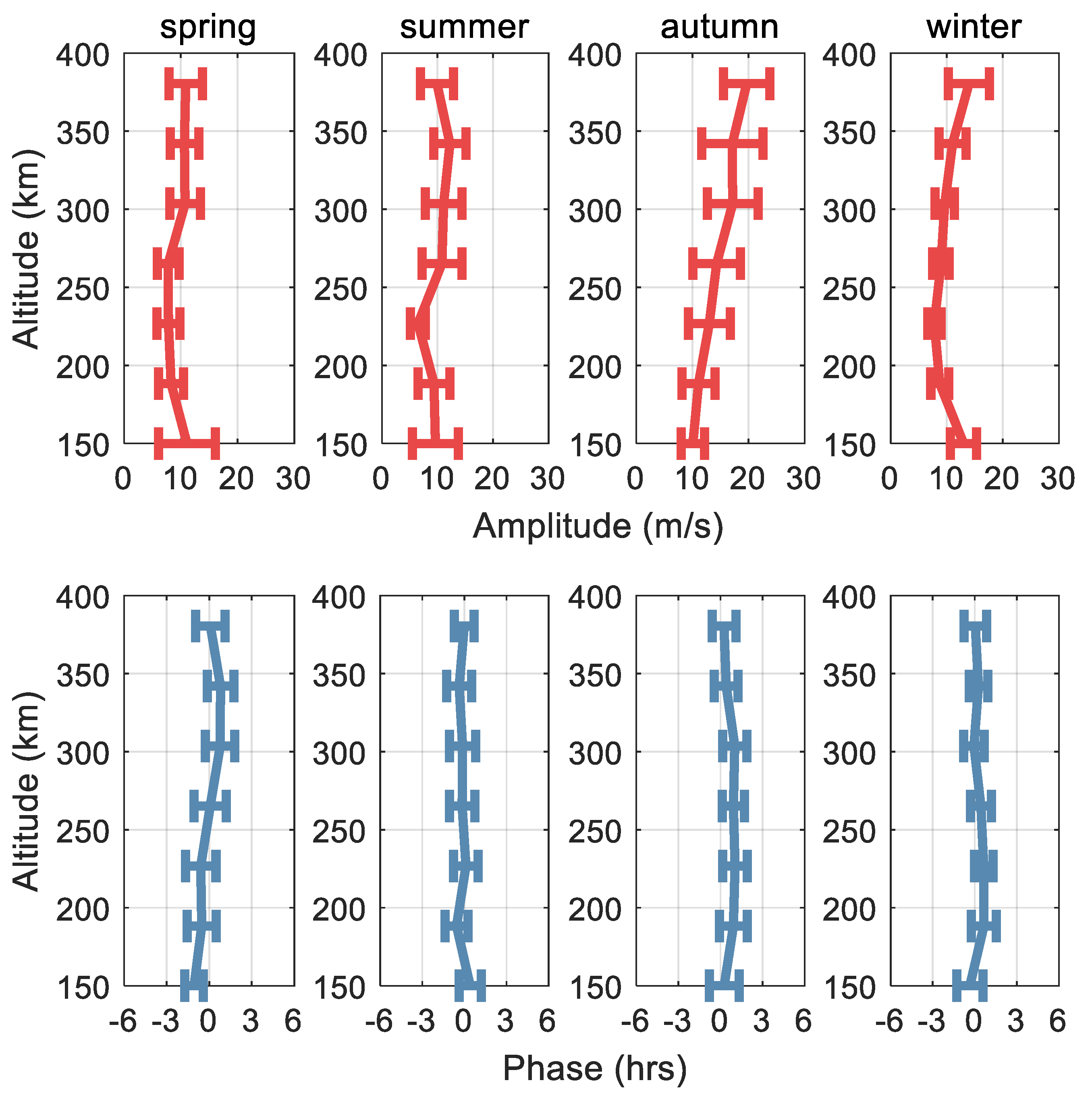
  • The amplitude of the 6 h oscillation is most prominent in autumn with a maximum amplitude of 20 m/s at 380 km, and it exhibits a clear pattern of increasing amplitude with height. The mean amplitude of the 6 h oscillations in the other seasons is 10 m/s. The vertical phase structures in the four seasons are largely consistent above 180 km, and they exhibit limited vertical variation.
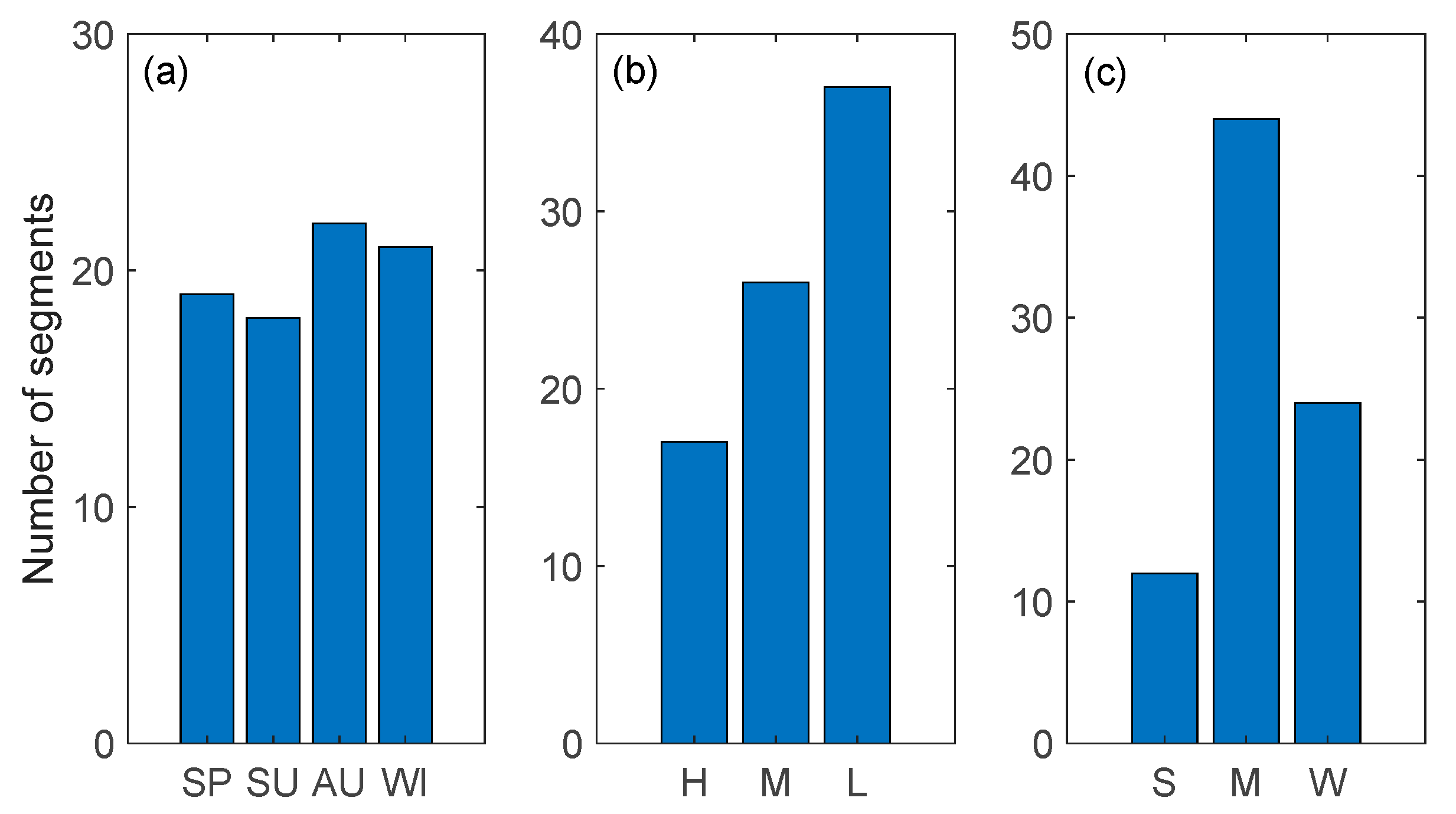
  • The mean amplitude of the 6 h oscillation is 10 m/s, 10 m/s, and 12 m/s under high, moderate, and low solar activities, respectively. Our results indicate that solar activities have a small effect on the thermospheric 6 h oscillation at Arecibo. Compared with the phenomenon wherein the thermospheric terdiurnal tide at low latitude has limited response to solar activities, tidal waves with shorter periods are likely not sensitive to solar activities.
  • The mean amplitude of the 6 h oscillation is 14 m/s, 12 m/s, and 10 m/s under strong, moderate, and weak geomagnetic activities. Above 250 km, the amplitude during strong geomagnetic activities is almost twice that occurring during weak geomagnetic activities. Our results indicate that the mean amplitude of the 6 h oscillation at low latitude increases with the intensification of geomagnetic activities above 200 km. Note that since the number of samples collected for strong geomagnetic activity is smaller than the number of the samples gathered for the moderate and weak geomagnetic activities, our conclusion may have a bias.

Author Contributions

Conceptualization, Y.G.; methodology, Y.G.; software, X.C.; validation, Y.D., X.C., Z.M. and J.L.; formal analysis, Y.D. and X.C.; investigation, Y.D. and X.C.; resources, Y.G.; data curation, Q.Z.; writing—original draft preparation, Y.G. and Y.D.; writing—review and editing, Y.G., S.Z. and Q.Z.; funding acquisition, Y.G., S.Z. and Q.Z. All authors have read and agreed to the published version of the manuscript.

Funding

This research was funded by the National Natural Science Foundation of China (42374192), the National Key R&D Program of China (2022YFF0503703), the National Youth Talent Support Program, and the National Science Foundation of United States AGS-2152109.

Data Availability Statement

The Arecibo ISR data can be found in the Madrigal Database at http://madrigal.iggcas.ac.cn/list/ (accessed on 1 January 2023).

Acknowledgments

We acknowledge the use of the Arecibo incoherent scatter radar data.

Conflicts of Interest

The authors declare no conflict of interest.

References

  1. Lindzen, R.S. The application of classical atmospheric tidal theory. Proc. R. Soc. 1968, 303, 299–316. [Google Scholar]
  2. Chapman, S.; Lindzen, R.S. Atmospheric Tides: Thermal and Gravitational; D. Reidel: Dordrecht, The Netherlands, 1970. [Google Scholar]
  3. Forbes, J.M.; Garret, H.B. Thermal excitation of atmospheric tides due to insolation absorption by O3 and H2O. Geophys. Res. Lett. 1978, 5, 12. [Google Scholar] [CrossRef]
  4. Forbes, J.M. Tidal and planetary waves. In The Upper Mesosphere and Lower Thermosphere: A Review of Experiment and Theory, Geophys; Geophysical Monograph Series; American Geophysical Union: Washington, DC, USA, 1995; Volume 87, pp. 67–87. [Google Scholar]
  5. Forbes, J.M.; Wu, D. Solar tides as revealed by measurements of mesosphere temperature by the MLS experiment on UARS. J. Atmos. Sci. 2006, 63, 1776–1797. [Google Scholar] [CrossRef]
  6. Lieberman, R.S.; Oberheide, J.; Talaat, E.R. Nonmigrating diurnal tides observed in global thermospheric winds. J. Geophys. Res. Space Phys. 2013, 118, 7384–7397. [Google Scholar] [CrossRef]
  7. Hagan, M.E.; Roble, R.G.; Hackney, J. Migrating thermospheric tides. J. Geophys. Res. 2001, 106, 12739–12752. [Google Scholar] [CrossRef]
  8. Hagan, M.E.; Forbes, J.M. Migrating and nonmigrating diurnal tides in the middle and upper atmosphere excited by tropospheric latent heat release. J. Geophys. Res. 2002, 107, 4754. [Google Scholar] [CrossRef]
  9. Gong, Y.; Zhou, Q. Incoherent scatter radar study of the terdiurnal tide in the E and F-region heights at Arecibo. Geophys. Res. Lett. 2011, 38, L15101. [Google Scholar] [CrossRef]
  10. Kumar, G.K.; Singer, W.; Oberheide, J.; Grieger, N.; Batista, P.P. Diurnal tides at low latitudes: Radar, satellite, and model results. J. Atmos. Sol. Terr. Physis 2014, 118, 96–105. [Google Scholar] [CrossRef]
  11. Gong, Y.; Zhou, Q.; Zhang, S. Atmospheric tides in the low-latitude E and F regions and their responses to a sudden stratospheric warming event in January 2010. J. Geophys. Res. Space Phys. 2013, 118, 5177–5183. [Google Scholar] [CrossRef]
  12. Gong, Y.; Xue, J.; Ma, Z.; Zhang, S.; Zhou, Q.; Huang, C.; Huang, K.; Yu, Y.; Li, G. Strong quarterdiurnal tides in the mesosphere and lower thermosphere during the 2019 arctic sudden stratospheric warming over Mohe, China. J. Geophys. Res. Space Phys. 2021, 10, 126. [Google Scholar] [CrossRef]
  13. Pedatella, N.M.; Oberheide, J.; Sutton, E.K.; Liu, H.L.; Anderson, J.L.; Raeder, K. Short-term nonmigrating tide variability in the mesosphere, thermosphere, and ionosphere. J. Geophys. Res. Space Phys. 2016, 121, 3621–3633. [Google Scholar] [CrossRef]
  14. Vitharana, A.; Du, J.; Zhu, X.; Oberheide, J.; Ward, W.E. Numerical prediction of the migrating diurnal tide total variability in the mesosphere and lower thermosphere. J. Geophys. Res. Space Phys. 2021, 126, e2021JA029588. [Google Scholar] [CrossRef]
  15. Guharay, A.; Batista, P.P.; Andrioli, V.F. Investigation of solar cycle dependence of the tides in the low latitude MLT using meteor radar observations. J. Atmos. Sol. Terr. Phys. 2019, 193, 105083. [Google Scholar] [CrossRef]
  16. Lee, J.; Kwak, Y.S.; Eswaraiah, S.; Kam, H.; Kim, Y.H.; Lee, C.; Kim, J.H. Observational evidence of nonlinear wave-wave interaction over Antarctic MLT region. J. Geophys. Res. Space Phys. 2023, 128, e2022JA030738. [Google Scholar] [CrossRef]
  17. Jacobi, C.; Krug, A.; Merzlyakov, E. Radar observations of the quarterdiurnal tide at midlatitudes: Seasonal and long-term variations. J. Atmos. Sol. Terr. Physis 2017, 163, 70–77. [Google Scholar] [CrossRef]
  18. Jacobi, C.; Geissler, C.; Lilienthal, F.; Krug, A. Forcing mechanisms of the 6h tide in the mesosphere/lower thermosphere. Adv. Radio Sci. 2018, 16, 141–147. [Google Scholar] [CrossRef]
  19. Guharay, A.; Batista, P.P.; Buriti, R.A.; Schuch, N.J. On the variability of the quarter-diurnal tide in the MLT over Brazilian low-latitude stations. Earth Planet Space 2018, 70, 140. [Google Scholar] [CrossRef]
  20. Pancheva, D.; Mukhtarov, P.; Hall, C.; Smith, A.; Tsutsumi, M. Climatology of the short-period (8-h and 6-h) tides observed by meteor radars at Tromsø and Svalbard. J. Atmos. Sol. Terr. Phy. 2021, 212, 105513. [Google Scholar] [CrossRef]
  21. Hindly, N.P.; Mitchell, N.J.; Cobbett, N.; Smith, A.K.; Fritts, D.C.; Janches, D. Radar observations of winds, waves and tides in the mesosphere and lower thermosphere over South Georgia island (54° S, 36° W) and comparison with WACCM simulations. Atmos. Chem. Phys. 2022, 22, 9435–9459. [Google Scholar] [CrossRef]
  22. Kovalam, S.; Vincent, R.A. Intradiurnal wind variations in the midlatitude and high-latitude mesosphere and lower thermosphere. J. Geophys. Res. 2003, 108, 4135–4147. [Google Scholar] [CrossRef]
  23. Liu, R.; Lu, D.; Yi, F.; Hu, X. Quadratic nonlinear interactions between atmospheric tides in the mid-latitude winter lower thermosphere. J. Atmos. Sol. Terr. Phys. 2006, 68, 1245–1259. [Google Scholar] [CrossRef]
  24. She, C.Y.; Chen, S.; Williams, B.P.; Hu, Z.; Krueger, D.; Hagan, M.E. Tides in the mesopause region over Fort Collins, Colorado based on lidar temperature observations covering full diurnal cycles. J. Geophys. Res. 2002, 107, 4350. [Google Scholar] [CrossRef]
  25. Walterscheid, R.L.; Sivjee, G.G. Very high frequency tides observed in the airglow over Eureka. Geophys. Res. Lett. 1996, 23, 3651–3654. [Google Scholar] [CrossRef]
  26. Walterscheid, R.L.; Sivjee, G.G. Zonally symmetric oscillations observed in the airglow from South Pole station. J. Geophys. Res. 2001, 106, 3645–3654. [Google Scholar] [CrossRef]
  27. Xu, J.; Smith, A.K.; Jiang, G.; Yuan, W.; Gao, H. Features of the seasonal variation of the semidiurnal, terdiurnal and 6-h components of ozone heating evaluated from Aura/MLS observations. Ann. Geophys. 2012, 30, 259–281. [Google Scholar] [CrossRef]
  28. Xu, J.; Smith, A.K.; Liu, M.; Liu, X.; Gao, H.; Jiang, G.; Yuan, W. Evidence for nonmigrating tides produced by the interaction between tides and stationary planetary waves in the stratosphere and lower mesosphere. J. Geophys. Res. Atmos. 2014, 119, 471–489. [Google Scholar] [CrossRef]
  29. Liu, M.H.; Xu, J.Y.; Yue, J.; Jiang, G.Y. Global structure and seasonal variations of the migrating 6-h tide observed by SABER/TIMED. Sci. China Earth Sci. 2015, 58, 1216–1227. [Google Scholar] [CrossRef]
  30. Azeem, I.; Walterscheid, R.L.; Crowley, G.; Bishop, R.L.; Christensen, A.B. Observations of the migrating semidiurnal and quaddiurnal tides from the RAIDS/NIRS instrument. J. Geophys. Res. Space Phys. 2016, 121, 4626–4637. [Google Scholar] [CrossRef]
  31. Jacobi, C.; Arras, C.; Geissler, C.; Lilienthal, F. Quarterdiurnal signature in sporadic E occurrence rates and comparison with neutral wind shear. Ann. Geophys. 2019, 37, 273–288. [Google Scholar] [CrossRef]
  32. Smith, A.K.; Pancheva, D.V.; Mitchell, N.J. Observations and modeling of the 6-hour tide in the upper mesosphere. J. Geophys. Res. 2004, 109, D10105. [Google Scholar] [CrossRef]
  33. Geissler, C.; Jacobi, C.; Lilienthal, F. Forcing mechanisms of the migrating quarterdiurnal tide. Ann. Geophys. 2020, 38, 527–544. [Google Scholar] [CrossRef]
  34. Tong, Y.U.; Mathews, J.D.; Ying, W.P. An upper E region quarterdiurnal tide at Arecibo. J. Geophys. Res. 1988, 93, 10047–10051. [Google Scholar] [CrossRef]
  35. Gong, Y.; Ma, Z.; Lv, X.; Zhang, S.; Zhou, Q.; Aponte, N.; Sulzer, M. A study on the quarterdiurnal tide in the thermosphere at Arecibo during the February 2016 sudden stratospheric warming event. Geophys. Res. Lett. 2018, 45, 13142–13149. [Google Scholar] [CrossRef]
  36. Gordon, W. Incoherent scattering of radio waves by free electrons with applications to space exploration by radar. Proc. IRE. 1958, 46, 1824–1829. [Google Scholar] [CrossRef]
  37. Sulzer, M. A phase modulation technique for a sevenfold statistical improvement in incoherent scatter data-taking. Radio Sci. 1986, 21, 737–744. [Google Scholar] [CrossRef]
  38. Isham, B.; Tepley, C.A.; Sulzer, M.P.; Zhou, Q.H.; Kelley, M.C.; Friedman, J.; Gonzalez, S. Upper atmospheric observations at the Arecibo Observatory: Examples obtained using new capabilities. J. Geophys. Res. 2000, 105, 18609–18637. [Google Scholar] [CrossRef]
  39. Sulzer, M.; Aponte, N.; Gonzalez, S. Application of linear regularization methods to Arecibo vector velocities. J. Geophys. Res. Space Phys. 2005, 110, A10. [Google Scholar] [CrossRef]
  40. Cai, X.; Burns, A.G.; Wang, W.; Qian, L.; Solomon, S.C.; Eastes, R.W.; Pedatella, N.; Daniell, R.E.; McClintock, W.E. The two-dimensional evolution of thermospheric ∑O/N2 response to weak geomagnetic activity during solar-minimum observed by GOLD. Geophys. Res. Lett. 2020, 47, e2020GL088838. [Google Scholar] [CrossRef]
  41. Aponte, N.; Nicolls, M.J.; González, S.A.; Sulzer, M.P.; Kelley, M.C.; Robles, E.; Tepley, C.A. Instantaneous electric field measurements and derived neutral winds at Arecibo. Geophys. Res. Lett. 2005, 32, L12107. [Google Scholar] [CrossRef]
  42. Buonsanto, M. Ionospheric storms—A review. Space Sci. Rev. 1999, 88, 563–601. [Google Scholar] [CrossRef]
  43. Gong, Y.; Lv, X.; Zhang, S.; Zhou, Q.; Ma, Z. Climatology and seasonal variation of the thermospheric tides and their response to solar activities over Arecibo. J. Atmos. Sol. Terr. Phys. 2021, 215, 105592. [Google Scholar] [CrossRef]
Figure 1. (a) The number of segments observed with 6 h oscillations in spring (SP), summer (SU), autumn (AU), and winter (WI); (b) the number of segments observed with 6 h oscillations under high (H), moderate (M), and low (L) solar activities; (c) The number of samples observed with 6 h oscillations under strong (S), moderate (M), and weak (W) geomagnetic activities.
Remotesensing 15 05098 g001
Figure 2. The temporal and altitudinal variations in the meridional wind from 16:00 LT 17 November to 12:00 LT 20 November 2005 and from 150 to 400 km.
Remotesensing 15 05098 g002
Figure 3. The climatological mean amplitude (red) and phase (blue) variations in the 6 h oscillation in the meridional wind in the thermosphere. The standard deviations of the climatological average are represented by error bars.
Remotesensing 15 05098 g003
Figure 4. The vertical variations in 6 h oscillational amplitudes (red) and phases (blue) in spring, summer, autumn, and winter, respectively. The standard deviations of the seasonal average are represented by error bars.
Remotesensing 15 05098 g004
Figure 5. The amplitude (red) and phase (blue) variations in the 6 h oscillations in the meridional wind under high (F10.7 ≥ 140 SFU, left column), moderate (100 SFU ≤ F10.7 < 140 SFU, medium column), and low (F10.7 < 100 SFU, right column) solar activities. The standard deviations of the average during different solar activities are represented by error bars.
Remotesensing 15 05098 g005
Figure 6. The amplitude (red) and phase (blue) variations in the 6 h oscillations in the meridional wind under strong (KP ≥ 4, left column), moderate (2 ≤ KP < 4, medium column), and weak (KP < 2, right column) geomagnetic storm activities. The standard deviations of the average during different geomagnetic activities are represented by error bars.
Remotesensing 15 05098 g006
Figure 7. (a) The phase variations in 6 h oscillations at 300 km from 17 to 20 November 2005; (b) the result of the superposed epoch analysis for the time interval of 17 to 20 November 2005.
Remotesensing 15 05098 g007
Disclaimer/Publisher’s Note: The statements, opinions and data contained in all publications are solely those of the individual author(s) and contributor(s) and not of MDPI and/or the editor(s). MDPI and/or the editor(s) disclaim responsibility for any injury to people or property resulting from any ideas, methods, instructions or products referred to in the content.

