Abstract
Drifting icebergs present significant navigational and operational risks in remote offshore regions, particularly along the East Coast of Canada. In such areas with harsh weather conditions, traditional methods of monitoring and assessing iceberg-related hazards, such as aerial reconnaissance and shore-based support, are often unfeasible. As a result, satellite-based monitoring using Synthetic Aperture Radar (SAR) imagery emerges as a practical solution for timely and remote iceberg classifications. We utilize the C-CORE/Statoil dataset, a labeled dataset containing both ship and iceberg instances. This dataset is derived from dual-polarized Sentinel-1. Our methodology combines state-of-the-art deep learning techniques with comprehensive feature selection. These features are coupled with machine learning algorithms (neural network, LightGBM, and CatBoost) to achieve accurate and efficient classification results. By utilizing quantitative features, we capture subtle patterns that enhance the model’s discriminative capabilities. Through extensive experiments on the provided dataset, our approach achieves a remarkable accuracy of 95.4% and a log loss of 0.11 in distinguishing icebergs from ships in SAR images. The introduction of additional ship images from another dataset can further enhance both accuracy and log loss results to 96.1% and 0.09, respectively.
1. Introduction
Ship/iceberg discrimination is crucial for maritime safety and efficiency. It helps with collision prevention, route optimization, and improves situational awareness to better manage vessel traffic in ice-infested waters. This ensures secure and effective maritime operations [1]. Synthetic Aperture Radar (SAR) is an active remote sensing technique that employs radar signals to generate high-resolution images of the Earth’s surface [2]. With the capacity to penetrate cloud cover and continuously monitor marine regions, SAR proves indispensable for ship and iceberg detection [3]. SAR uses microwave pulses to create detailed images by capturing reflected signals. Ships and icebergs have distinct shapes and materials that cause them to reflect radar signals differently. This distinction enables the accurate differentiation between ships and icebergs [4,5]. SAR target detection aims to swiftly and effectively identify the orientation and location of the target within complex scenes [6].
Deep learning (DL) has rapidly evolved and demonstrated successful applications in various fields, including signal and image processing, for tasks such as target detection in SAR images [7,8]. DL typically requires a substantial dataset for effective training, but the scarcity of SAR data poses a challenge. As a result, much of the research on SAR image processing has shifted towards transfer learning [9,10,11]. Transfer learning is a DL method that leverages the weights of a pre-trained model and fine tunes it for a specific application using a relatively small dataset [12].
The Convolutional Neural Network (CNN) is a widely used DL method for computer vision tasks, which are capable of effectively extracting low- and high-dimensional image features due to their hierarchical structure [13]. Researchers have relied more heavily on CNNs for SAR image target detection. The specific imaging mechanisms of SAR introduce clutter and noise, which can complicate the feature extraction process. Nevertheless, CNN’s deep feature extraction structure and robust capabilities make it well-suited for SAR image processing tasks [14]. Ref. [15] employed a DCN-based spatial feature extraction to enhance parcel-based crop classifications in SAR images. The authors in [16] presented a fusion method based on a CNN for extracting features from Sentinel data. In [17], the ResNet model and transfer learning were applied to a general SAR ship dataset, resulting in an average detection accuracy of 94.7%.
Numerous studies have extensively explored marine target detection, such as ships and icebergs, in SAR imagery, employing various methodologies. Constant False Alarm Rate (CFAR) algorithms are widely utilized for target detection in SAR images to effectively minimize false detections [18]. The algorithm that combines CFAR and CNN is more suitable for application in the ship detection system because it offers higher accuracy, a faster detection speed, and achieves ideal detection results [19]. In [20], the authors proposed an integrated approach using a single-shot multi-box detector [21] and transfer learning with the VGG16 model to detect ships in complex backgrounds. The model was tested on Sentinel-1 SAR images with VH/VV polarization and achieved a high detection accuracy. Region-based CNN (R-CNN) and You Only Look Once (YOLO) models, along with their variants, have been extensively employed for ship detection in SAR images [22,23,24,25,26]. These methods not only detect ships accurately, but also provide precise bounding boxes around the detected objects.
Related Works: SAR images have recently been used for discriminating icebergs from ships to avoid collisions between them [27]. In [28], H. Heiselberg suggested two CNN models and a Support Vector Machine (SVM) [29] for ship–iceberg classifications and obtained an accuracy of 86% for SAR and 94% for Multispectral Satellite Image (MSI) datasets. P. Heiselberg and et al. proposed a new CNN model for the ice/ship discrimination with an accuracy of 93% [30]. In [31], DenseNet and ResNet were deployed for feature extraction and image classification directly on original SAR images. Additionally, texture features were extracted from de-speckled SAR images, followed by a classification using XGBoost [32] and LightGBM [33], resulting in a high accuracy. Another feature-based approach was proposed in [34], where a supervised search and classification algorithm was designed based on the physical parameters to identify and categorize objects in the sea with reflectance values exceeding a predefined threshold. The algorithm achieved an accurate discrimination, surpassing a 90% precision score, among various objects, such as ships, islands, wakes, icebergs, ice floes, and clouds.
In this paper, we propose a CNN-based feature extraction method using VGG16, ResNet50, and ConvNeXtSmall models. The best 300 features extracted by these CNN models are then combined with quantitative (statistical and spatial) features for each band. Subsequently, all these features are classified using various machine learning methods, such as NN, LightGBM, and CatBoost [35]. The outputs of these classifiers are eventually combined using a decision tree.
Contribution: This paper makes two noteworthy contributions to the current body of literature. Firstly, it extracts an extensive set of features from various pre-trained CNNs. Subsequently, a method is employed to reduce the dimensionality of the feature vector by discarding weaker features based on their mutual information with image labels and selecting the most effective features. Furthermore, this research incorporates additional statistical and spatial features, after demonstrating their efficiency in distinguishing between ships and icebergs.
The rest of this paper is organized as follows: Section 2 outlines the materials, such as the dataset and machine-learning models employed in this research, while Section 3 presents the proposed method. Section 4 discusses the results obtained for various datasets. The paper is concluded in Section 5.
2. Materials and Methods
2.1. Datasets
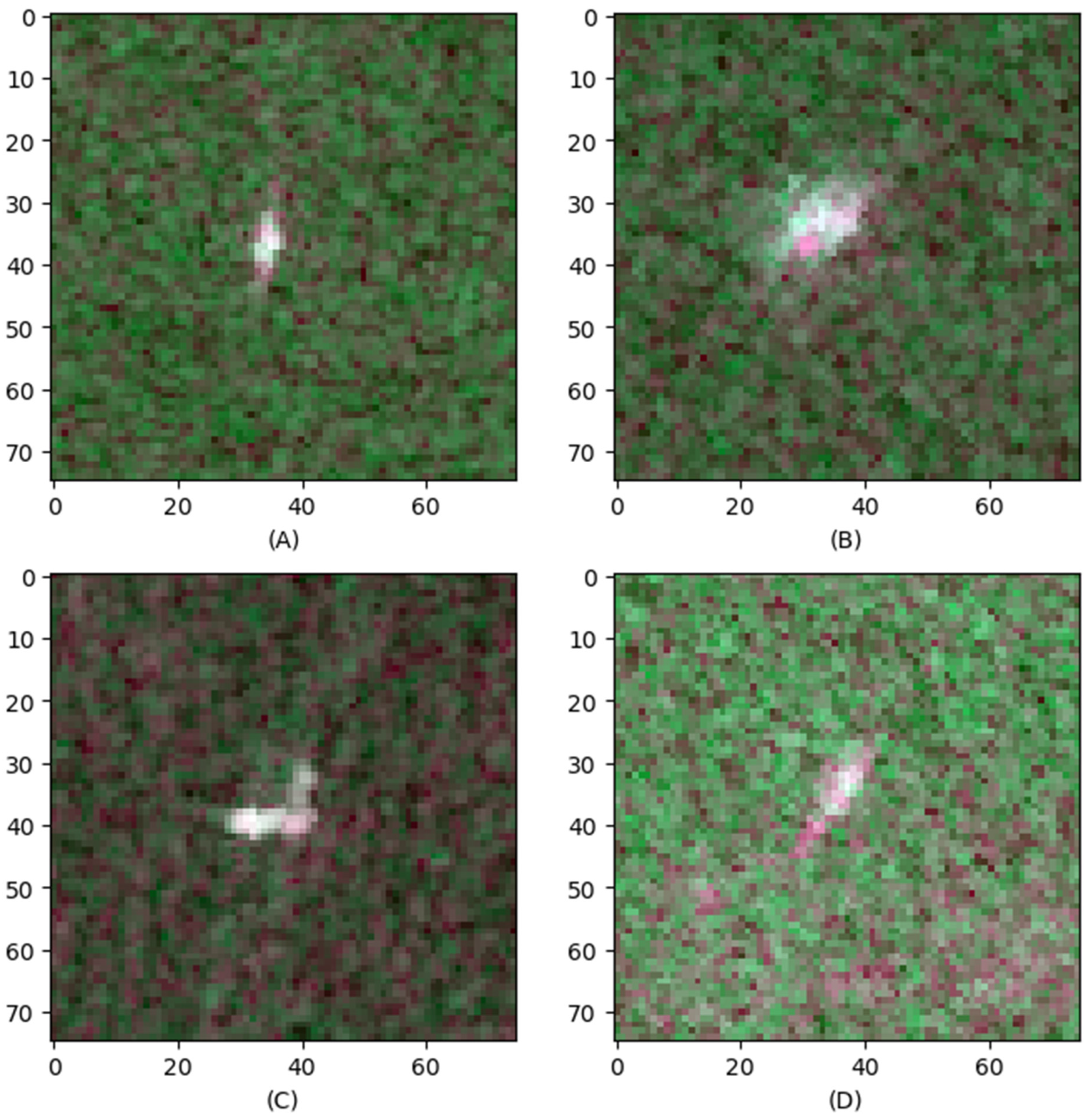
- The main dataset for this project was sourced from a Kaggle competition [36] and comprised 1604 images, depicting 851 ships and 753 icebergs. These images were SAR images captured by the Sentinel-1 satellite, with a 10-m pixel spacing. This enhanced resolution was crucial for detecting smaller ships accurately. The Sentinel-1 SAR operates with two dual polarizations, featuring HH (horizontal transmit, horizontal receive) and HV (horizontal transmit, vertical receive) bands within each scene. Human experts and geographical knowledge contributed to the labeling of the dataset. The image size for each band was 75 × 75 pixels. Notably, the intensity values for both HH and HV bands were represented in decibels (dB) and were flattened into one-dimensional vectors. Figure 1 depicts four sample images of the dataset.
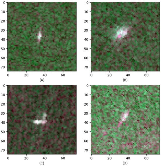 Figure 1. Four sample RGB images from the SAR dataset, where R = HH, G = HV, and B = (HH + HV)/2. (A,C) are ships, and (B,D) are icebergs.
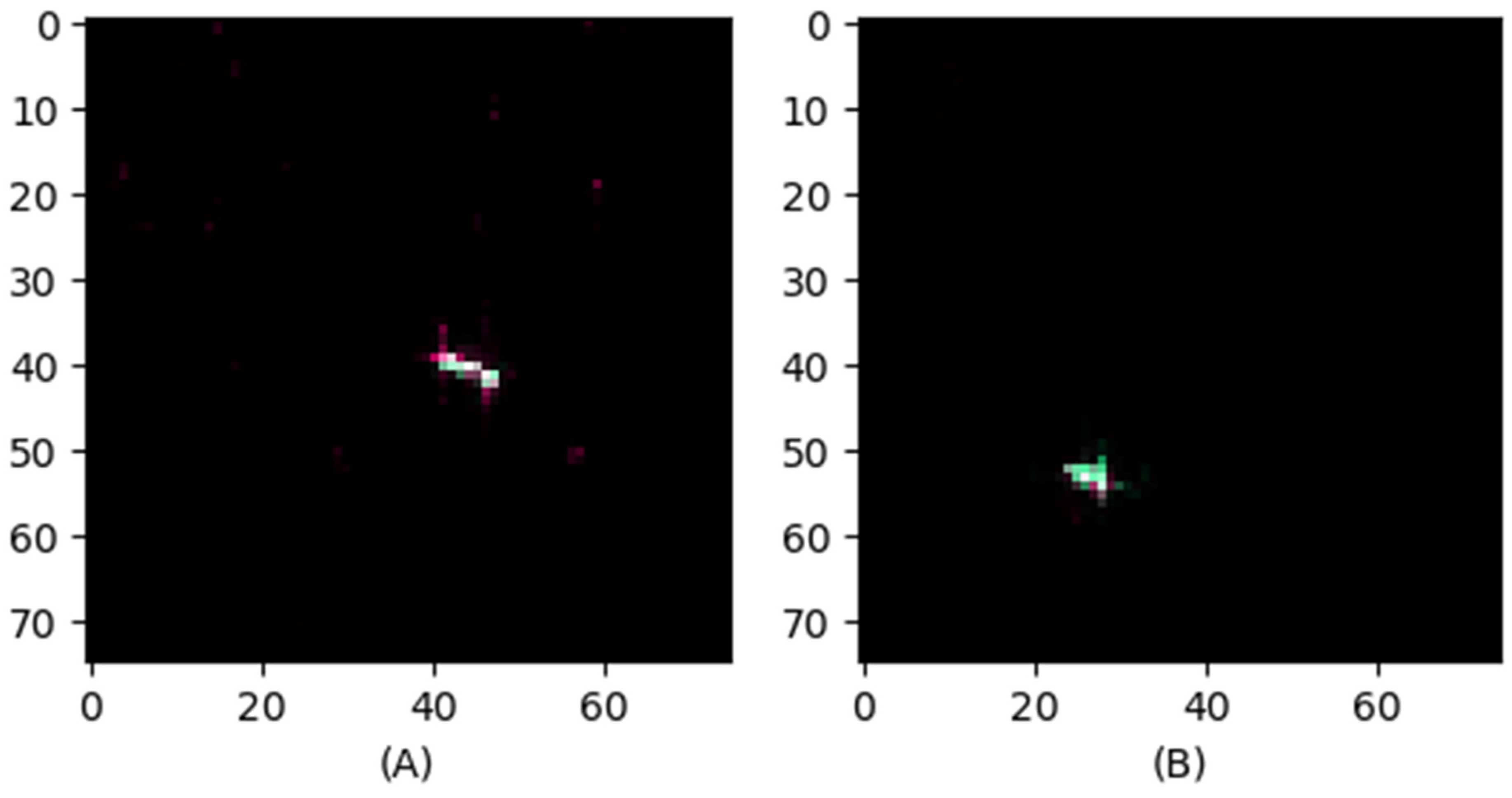
 - The SAR Ship Detection Dataset (SSDD) stands as the pioneering, openly available dataset extensively employed for exploring state-of-the-art ship detection technology using DL from the SAR images [37]. The dataset had 39,729 images, including 17,648 HH and 14,713 HV images, where 4911 of them had both HH and HV images that were used in our research, which required both HH and HV bands. Since this dataset only provided ship images, in order to keep our data relatively balanced, we selected and combined 1000 of these pairs of HH and HV images with the SAR data. Figure 2 illustrates two sample images from this dataset. A summary of both datasets are presented in Table 1.
 Figure 2. (A,B) Two sample RGB images of ships drawn from the SSDD dataset, where R = HH, G = HV, and B = (HH + HV)/2.
 Table 1. Description of Sentinel-1 and SSDD datasets.
2.2. Models
- Visual Geometry Group 16 (VGG16) [38] is a CNN architecture that gained significant attention and recognition for its role in image classification and deep learning research. VGG16 is characterized by its deep architecture, consisting of 16 layers, including 13 convolutional layers and 3 fully connected layers utilizing small 3 × 3 convolutional filters throughout the network, which contributes to its depth and effectiveness in capturing hierarchical features from images. VGG16 has been known to have the best classification accuracy, but since its architecture consists of approximately 138 million weights, it might not be the most computationally efficient model. In this project, the features were extracted from the output of the second Fully Connected (FC) layer, which was the last layer before the classification layer and included 4096 nodes.
- Residual Network 50 (ResNet-50) [18] is a sophisticated CNN structure that utilizes residual connections to address the vanishing gradient problem. With a total of 50 layers, it includes convolutional layers, batch normalization layers, ReLU activation functions, and fully connected layers. A noteworthy feature of ResNet-50 is its incorporation of skip connections, allowing the network to effectively capture both low- and high-level features by bypassing certain layers in the architecture. In this project, the features were extracted from the output of average pooling layer, which was the last layer before the classification layer with 2048 nodes.
- ConvNeXt [39] is a purely convolutional model designed to enhance the capabilities of convolutional neural networks by utilizing parallel branches for capturing distinct and supplementary features. This architecture, known for its varying number of layers, demonstrates a remarkable performance across a range of computer vision tasks, including image classification, object detection, and semantic segmentation. In this project, we used ConvNeXtSmall, which had 50 million parameters, and the features were extracted from the output of average pooling layer, which was the last layer before the classification layer and included 768 nodes.
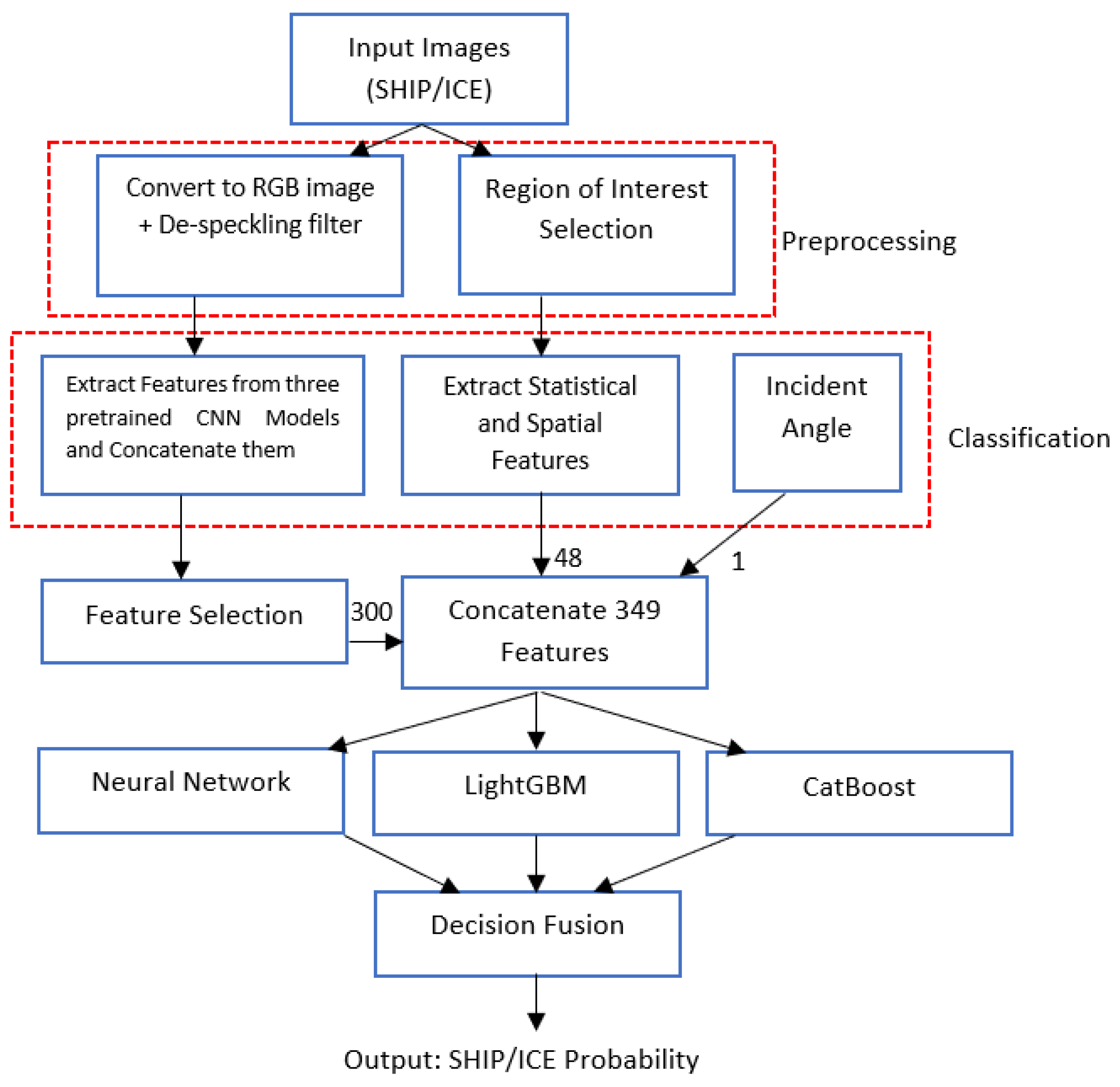
3. Proposed Method
In this paper, we modified the method outlined in [40], augmenting it with the inclusion of quantitative (statistical and spatial) features in addition to the CNN-based features obtained from various CNN models. The CNN features that were extracted were subsequently pruned, selecting only the best 300 features based on mutual information between the features and targets [41]. These selected features were then combined with the quantitative features, forming a concatenated feature set. This composite feature set was utilized for the classification of ship and iceberg images. The system architecture is depicted in Figure 3. As depicted, images from different datasets underwent initial preprocessing, followed by parallel stages of feature extraction. The resultant features were then merged, and the classification was performed using three machine learning techniques: NN, LightGBM, and CatBoost. The resulting probabilities from these methods were aggregated through a decision tree to calculate the final log loss score. Further details regarding each component are elaborated below.
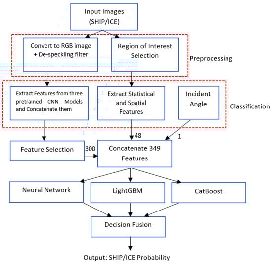
Figure 3.
Block diagram of the proposed system.
3.1. Preprocessing
For the SAR dataset, the decibel (dB) values of HH and HV polarizations were provided for each ship and iceberg instance, resulting in 2 vectors of 5625 values each, corresponding to the 5625 pixels. Preprocessing is different between CNN and quantitative features: CNN requires normalized RGB images, while our quantitative features rely on raw dB values for an improved performance, and therefore, additional preprocessing, such as despeckling affects the signal statistical parameters useful for the classification. To transform these values into CNN-compatible RGB images, the vectors were initially assigned to the R, G, and B channels as R = HH, G = HV, and B = (HH + HV)/2. Subsequently, each channel was scaled to the 0 to 255 range and reshaped to a 75 × 75 pixel format. A further enhancement was performed by filtering the RGB images with bilateral and Lee despeckling filters, as demonstrated in Figure 4. As one can see, both filters smooth the background; however, the bilateral filter does not preserve the details of the targets. Hence, in this paper, the Lee filter was used for preprocessing the images.
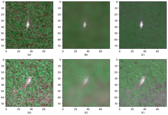
Figure 4.
The effect of despeckling using bilateral and Lee filters on samples of ship and iceberg images from the SAR dataset. (A,D) illustrate two sample images of a ship and iceberg before filtering, (B,E) present similar images for a ship and iceberg after bilateral filtering, and (C,F) show them after Lee filtering, respectively.
3.2. Feature Extraction
3.2.1. CNN Features
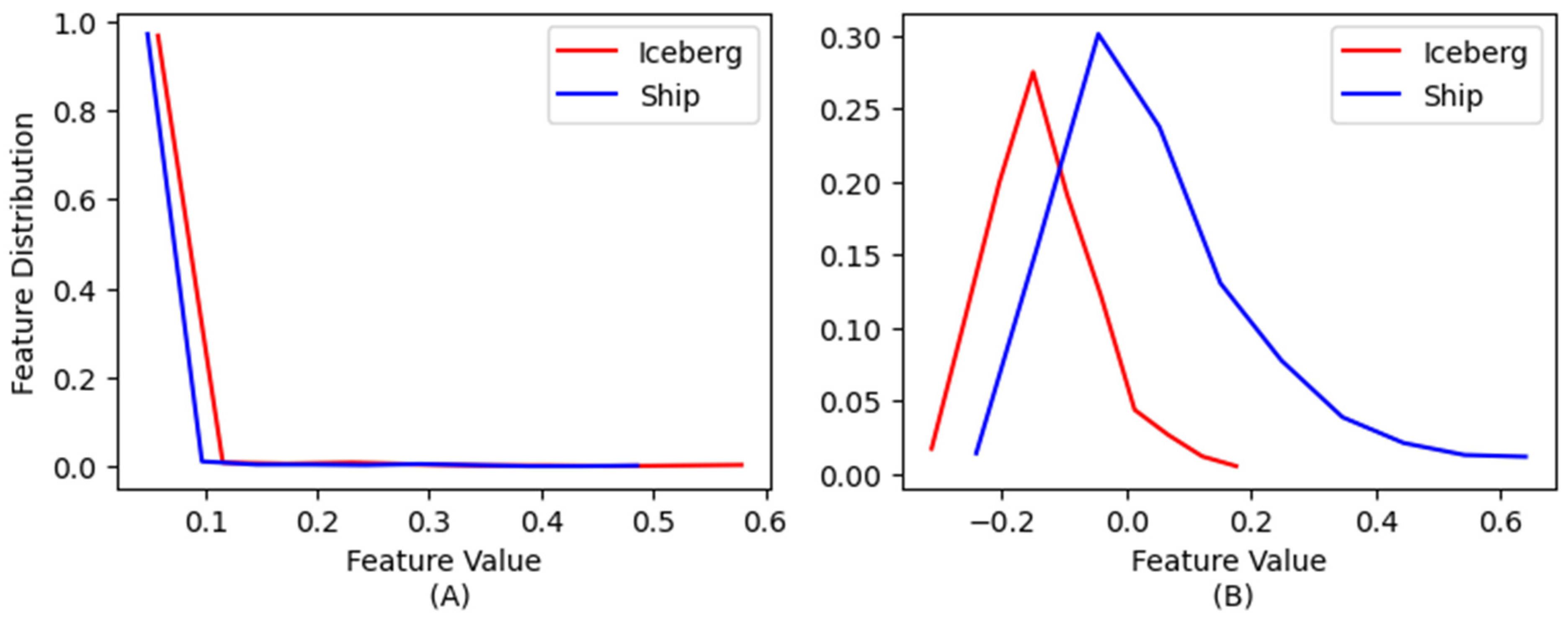
To extract the CNN features, we used three CNN models, described in Section 2.2. We selected these three models after an extensive search over various CNN models based on their performance. We totally extracted 6912 features: 4096 from VGG16, 2048 from ResNet50, and 768 from the ConvNeXtSmall models. Table 2 presents the name of the layer in tensorflow from where the features were extracted and the number of each feature in each CNN model. Most of these features did not provide useful information and could thus be removed from the feature set. This not only reduced the complexity of the classifier, but also improved its performance. Figure 5 depicts two histograms of sample CNN features extracted from ships and icebergs individually. These features were chosen based on their mutual information. Figure 5A represents the histograms of a weak feature, as evidenced by the complete overlap in its histograms and a computed mutual information value between a feature and target of zero. In contrast, Figure 5B represents the histograms of a strong feature with distinctive histograms, providing a mutual information value as high as 0.165. This observation motivated us to reduce the number of features based on the mutual information between the features and target labels. We selected the best 300 features out of the total of 6912, considering those with the highest mutual information values.
Table 2.
CNN models used in the proposed method, along with the layer name where the features have been extracted and the number of features extracted from each model.
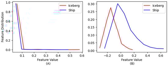
Figure 5.
These figures show distributions of (A) a weak feature and (B) a strong feature extracted using pre-trained CNN models for ship and iceberg images in the SAR dataset. The mutual information computed for these two features is zero and 0.165, respectively.
3.2.2. Quantitative (Statistical/Spatial) Features
To extract these features for both datasets, each band, HH, HV, and HH + HV, was processed individually. In the first step, we extracted the Region of Interest (ROI) for each band using the log-normal CFAR algorithm. To ensure that the foreground (either the ship or iceberg) was detected, we set the probability of false alarm (PFA) = 0.1. Then, the largest blob in the threshold image was obtained and used to mask out the target from the background, and the intensity values in the target area were used to compute the features. For each band, we computed 16 statistical/spatial features as follows:
Statistical Features:
The following statistical features were extracted from the raw values of each thresholded band, two additional bands that were obtained from the addition and subtraction of HH and HV bands:
1. Minimum intensity: the lowest pixel value in the image.
2. Maximum intensity: the highest pixel value in the image.
3. Mean intensity (μ): the average pixel value of all the pixels in the image.
4. Standard deviation of intensities: the standard deviation is a measure of the dispersion of pixel values around the mean.
where Σ is the summation symbol over the target area, x is each pixel value, and N is the number of pixels.
5. Skewness: the measure of the asymmetry of the probability distribution of a real-valued random variable and it is defined as
6. Kurtosis: the measure of the “tailedness” of the probability distribution of a real-valued random variable and it is defined as:
7. Randomness or uncertainty of a random variable:
where P(x) is the probability of occurrence of value x.
Spatial Features:
Since ships and icebergs have different shapes as, for instance, ships have more smooth and elongated boundaries and icebergs have more rough and round shapes, incorporating spatial features significantly improves the accuracy of classification. The spatial features used in the proposed method were as follows:
8. Area of the target: the area is the number of pixels that belong to the object in the image.
9. Perimeter of the target: the perimeter is the length of the boundary of the object in the image.
10. Ratio of the minimum axis of the target over its maximum: this ratio measures the elongation or compactness of the object and is calculated as Ratio = Minimum Axis/Maximum Axis.
11. Eccentricity of the target: eccentricity measures how much the shape of the object deviates from a perfect circle.
12. Hu moments: a set of seven mathematical moments that capture the shape and texture information in an image. They are invariant to translation, rotation, and scaling, making them useful for pattern recognition and image analysis [42]. In this paper, we used the first five hue moments for each band, as the values obtained from the last two moments were unreliable.
Analysis of quantitative (statistical and spatial) features:
We analyzed the effects of individual features by comparing histograms for each statistical and spatial attribute separately for ships and icebergs. This analysis helped us understand the influence of each feature on the overall classification performance. For instance, if the histograms for ships and icebergs showed a significant overlap with regard to a particular feature, it suggested that the feature provided limited valuable information for the classification of object labels. Consequently, its impact on the discrimination performance was minor. Conversely, if the histograms for ships and icebergs exhibited minimal overlap and distinctness for a specific feature, this indicated that the feature imparted valuable information related to the target label and contributed significantly to the overall performance. Figure 6, Figure 7, Figure 8 and Figure 9 depict the histograms of the features extracted from the ships and icebergs individually for the HH, HV, HH − HV, and HH + HV bands, respectively.
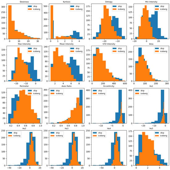
Figure 6.
Histogram of the features introduced in this section for ships (blue) and icebergs (orange) for the HH band.
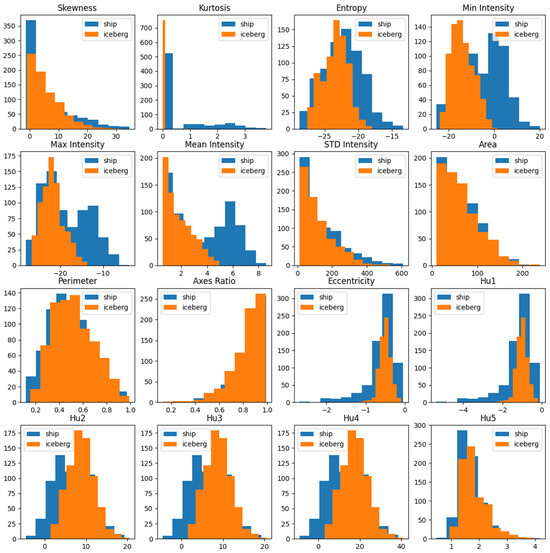
Figure 7.
Histogram of the features introduced in this section for ships (blue) and icebergs (orange) for the HV band.
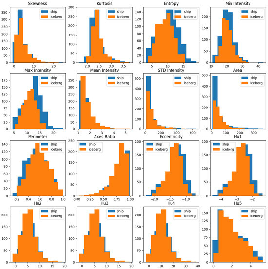
Figure 8.
Histogram of the features introduced in this section for ships (blue) and icebergs (orange) for the HH − HV band.
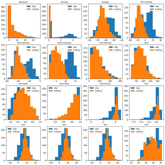
Figure 9.
Histogram of the features introduced in this section for ships (blue) and icebergs (orange) for the HH + HV band.
Table 3 presents the mutual information between each of the features and target labels calculated over the images. Figure 6, Figure 7, Figure 8 and Figure 9 illustrate the histograms of the features for the ships and icebergs, individually.
Table 3.
Mutual information between each statistical/spatial feature and target label (features that provide a significant contribution to classification accuracy are highlighted in bold).
From Table 3 and Figure 6, Figure 7, Figure 8 and Figure 9, we can see that, for the HH band, all the features, except the standard deviation (std), area, and skewness (sk), provide useful information as the histograms for the ships and icebergs are relatively distinctive. Kurtosis (ku), Max, Mean (avg), Entropy (ent), and Hu features provided distinctive information for HH, HV, and HH + HV, but they did not provide much information for HH − HV. We can also see that, for HH − HV, almost none of the features, except entropy, present useful information as all the histograms of the ships considerably overlap with the ones for the icebergs. Hence, we decided to proceed with the features excluded from HH, HV, and HH + HV, and excluded the features extracted from HH − HV. This result also justifies using these three bands as R, G, and B components of the color image used in the preprocessing stage, as mentioned in Section 3.1.
3.2.3. Incident Angle
One additional useful parameter is the incident angle, which exerts a notable influence on depolarization effects. The interaction of radar signals with different surface types and structures leads to a conversion of transmitted polarization states. The incident angle determines the prevalence of scattering mechanisms, such as surface, double bounce, and volume scattering, affecting the power distribution between HH and HV signals. This phenomenon results in angle-dependent changes in the power ratio between these polarizations, known as the depolarization ratio. Understanding these angle-dependent depolarization behaviors is crucial for the accurate classification of ship and iceberg targets and provides insights into their scattering characteristics, enhancing the effectiveness of radar-based classification approaches.
3.3. Feature Concatenation
The 300 selected features derived from three distinct CNN models were subsequently merged with 48 quantitative features originating from the HH, HV, and HH + HV bands, encompassing 16 features from each band. Furthermore, within the SAR dataset, the inclusion of incident angle information was feasible for 1471 out of 1604 images. This aggregation provided a total of 349 distinct features. It is noteworthy that the utilization of the incident angle data necessitated a reduction in the dataset size from 1604 to 1471 instances; however, this trade-off was justifiable owing to the pivotal significance of the incident angle in influencing the HH and HV signal values.
3.4. Feature Classification
After selecting the best features, we needed to classify them. For this purpose, we tried multiple machine learning classifiers, such as K-Nearest Neighbor (KNN), Random Forest (RF), SVM, NN, XGBoost, LightGBM, and CatBoost. After investigating these models over the SAR dataset, we achieved the best accuracy values for NN, CatBoost, and LightGBM, respectively. Therefore, we selected these three models and combined their soft (probability) output using a decision tree. The details of each of these classifiers is as follows:
- NN: in the NN method, we used two fully connected layers with a hidden layer, including 96 neurons and a single-neuron classification layer. To minimize the overfitting problem, we used the L2 norm kernel regularization with a factor of 0.01 and a drop-out layer with a parameter of 0.2. For the classification layer, we used a sigmoid activation function that provided the probability of the target being an iceberg.
- CatBoost: a robust gradient boosting classifier that employs a blend of ordered boosting and oblivious trees, alongside a novel strategy known as “ordered boosting.” It also incorporates innovations, like the “Bayesian bootstrap” technique, to enhance generalization [43]. Our efforts to enhance the model’s performance involved optimizing specific parameters: iterations = 500, depth = 6, learning rate = 0.2, border count = 125, and using log loss as the loss function. We selected the best values of depth and border count in order to minimize the overfitting problem. Default settings were retained for the remaining parameters, streamlining the process by reducing the requirement for extensive hyperparameter tuning.
- LightGBM: an advanced gradient boosting framework recognized for its effectiveness and adaptability in managing extensive datasets. Its distinguishing features include a novel histogram-based binning strategy, leading to faster training and decreased memory consumption [44]. To enhance our model’s effectiveness, we optimized specific parameters, such as the log loss metric, utilizing 31 leaves, a learning rate of 0.05, feature fraction of 0.9, and 200 boost rounds. Furthermore, for regularization, we set min child samples = 20 and depth = 6. Default settings were retained for the remaining parameters.
- Decision tree: after calculating the ship/iceberg probabilities using the three machine learning methods mentioned above, we utilized a single decision tree to fuse them and determine the final log loss. The decision tree classifier is a core classification algorithm that constructs a tree-like structure to classify the data based on their features [45]. In this study, as the tree involved only three inputs, we adopted the default parameter settings of the decision tree. These settings entailed using the Gini impurity as the splitting criterion, employing the ‘best’ strategy as the splitter, not imposing a maximum depth limit, and requiring a minimum of two samples for splitting the internal nodes.
4. Results and Discussion
This section presents the results obtained from the Sentinel-1 (SAR dataset) introduced in Section 2.1, utilizing the models described in Section 2.2, as well as a fusion of all the models, as illustrated in Figure 3. The proposed method was implemented with Python using TensorFlow package version 2.11. We employed accuracy as a metric to evaluate and compare the performance of the proposed models. Accuracy was determined by comparing the predicted labels with the ground truth, quantifying the ratio of correctly discriminated targets. The Kaggle competition utilized log loss as the scoring metric. Therefore, to ensure comparability with submissions to the competition, we also adopted log loss as an alternative performance metric. The calculation of the log loss score involves the predicted probabilities and the ground truth as follows:
where n is the number of images in the test set, m is the number of image class labels, equals 1 if observation i belongs to Class j and 0, and is the predicted probability that observation i belongs to Class j. The goal was to achieve a minimal log loss score.
4.1. Performance Evaluation of the Proposed Method for Different Models and Classifiers
In this section, we assess the performance of the proposed method for different CNN models and various classifiers using the SAR dataset. The comparison involved evaluating the outcomes from the top 300 features extracted from VGG16, ResNet50, and ConvNeXtSmall individually, as well as their concatenated form. These feature sets were subjected to classifications using three state-of-the-art classifiers. In the following step, we utilized the probabilities derived from the three classifiers and fused them through a decision tree. The decision tree automatically determined the optimal thresholds to maximize the accuracy of the combined predictions from the three models. We utilized a 10-fold cross-validation, involving ten rounds of training and testing. In each iteration, 90% of the data was used for training, while 10% was allocated for testing.
Table 4 presents a comparative analysis of the training classification accuracy for different CNN models and classifiers. As one can see, with the exception of the NN, all other classifiers achieved 100% accuracy on the training data, regardless of the model used. It is important to note that this table was designed to offer insights into the training behavior of each model. However, considering the significance of the testing data, we solely focused on the results obtained from the testing data.
Table 4.
Average training accuracy of the proposed method for different CNN models, different classifiers, and their combination.
Table 5 presents the accuracy and log loss averaged over 10-fold for the testing data, across various CNN models and classifiers. Among the individual CNN models, Resnet50 slightly outperformed the other models in terms of accuracy and log loss. Its superior performance can be attributed to the capability of the network to effectively learn complex features without encountering vanishing gradient problems. As one can see, concatenating the three models improves the accuracy of the testing data by about 1.4% more than the best individual model.
Table 5.
Average testing accuracy/log loss of the proposed method for different CNN models, different Classifiers and combination of them.
Table 6 demonstrates the results obtained from the proposed method for the quantitative features as well as their combinations with features extracted from the CNN models. As one can see from this table, 49 quantitative features alone provide an accuracy as high as 93.1% and a log loss value as low as 0.17 for the test data. This outcome is particularly interesting as the extraction of these features requires much lower computational power compared to CNN-based methods, while still achieving competitive results. Furthermore, we concatenated these features with the 300 best features extracted from the concatenated three CNN models and classified them using the same classifiers, along with their fusion based on a decision tree. This combination improved both the accuracy and log loss as an average accuracy of 95.4% was achieved. The results clearly demonstrate the efficiency of the proposed method.
Table 6.
Average testing accuracy/log loss of the proposed method for quantitative features and its combination with selected CNN features.
4.2. Comparison of the Proposed Method with Existing Methods
In this section, we compare the outcomes of our proposed method with those of the existing methods. While there are few publications on ship/iceberg classifications from the SAR images, to the best of our knowledge, only two of them employ the same dataset as ours. Table 7 presents the accuracy and log loss values for the proposed method and three state-of-the-art methods. Among these methods, the approach presented in [34] exhibited the best performance in terms of both accuracy and log loss. This superiority can be attributed to the substantial amount of data used in their method, incorporating nearly 100,000 images comprising 9810 ships and ten-times more icebergs.
Table 7.
Comparison of accuracy and log loss values with the existing methods.
However, despite the significantly smaller dataset used in our approach, superior results for both the accuracy and log loss are achieved. For our proposed method, we initially employed the SAR dataset, which involved 1471 images and provided incident angle information. With these data, we attained an accuracy as high as 95.4% and a log loss as low as 0.11. For the second experiment, we incorporated an additional 1000 ship images from the SSDD dataset. It is important to note that the SSDD data did not include the incident angle information, so we excluded the incident angle from our feature set for this dataset. Consequently, for this particular experiment, our dataset consisted of 2604 images, including 753 icebergs and 1851 ships.
It is worth mentioning that, if we were to introduce more images from the SSDD dataset, our combined dataset would become imbalanced, potentially leading to a prediction bias towards ships. With the combined dataset, our proposed algorithm achieved an impressive accuracy of 96.1% and a remarkably low log loss value of 0.09.
5. Conclusions
In this research, we proposed a novel method to address the problem of ship/iceberg classification in remote offshore areas, particularly along the East Coast of Canada. Our approach involved extracting features from three CNN models: VGG16, ResNet50, and ConvNeXtSmall. The best 300 of these features were selected based on the mutual information between each feature and the target label. Additionally, we incorporated 48 quantitative features, as well as the incident angle, to form a vector, including 349 features for each image. These features were classified using three different machine learning algorithms: Neural Network (NN), LightGBM, and CatBoost. The prediction probabilities obtained from these classifiers were further fused using a decision tree to yield the final target probability. The proposed method was compared with the relevant state-of-the-art methods and demonstrated a superior performance, achieving a classification accuracy of 95.4% with only the Kaggle dataset and 96.1% after adding 1000 ship images from the SSDD dataset.
The main contribution of this paper is the introduction of a method to eliminate weak features from a set of extensively extracted features, employing various techniques, including pre-trained CNN models. This technique not only reduces classifier complexity, but also enhances the classification performance, making it valuable and reproducible for other applications. Another significant contribution of this paper is the introduction of a set of quantitative features that incorporate statistical information and shape-related details for ships and icebergs.
Several directions for future studies were envisioned. These included the extraction of additional physical and spatial features, the collection of larger and new datasets from the RADARSAT Constellation Mission (RCM), and the development of techniques for the detection and tracking of ships and icebergs in ocean environments.
Author Contributions
Conceptualization, Z.J., E.K., P.B. and R.T.; methodology, Z.J. and E.K.; software, Z.J.; validation, Z.J. and E.K.; formal analysis, Z.J. and E.K.; investigation, P.B. and R.T.; resources, P.B.; writing—original draft preparation, Z.J. and E.K.; writing—review and editing, Z.J. and E.K.; visualization, Z.J.; supervision, P.B. and R.T.; project administration, P.B. and R.T.; funding acquisition, R.T. All authors have read and agreed to the published version of the manuscript.
Funding
This research received no external funding.
Data Availability Statement
Not applicable.
Conflicts of Interest
The authors declare no conflict of interest.
References
- Amani, M.; Mehravar, S.; Asiyabi, R.M.; Moghimi, A.; Ghorbanian, A.; Ahmadi, S.A.; Ebrahimy, H.; Moghaddam, S.H.; Naboureh, A.; Ranjgar, B.; et al. Ocean remote sensing techniques and applications: A review (part ii). Water 2022, 14, 3401. [Google Scholar] [CrossRef]
- Chan, Y.K.; Koo, V. An introduction to synthetic aperture radar (SAR). Prog. Electromagn. Res. B 2008, 2, 27–60. [Google Scholar] [CrossRef]
- Jawak, S.D.; Bidawe, T.G.; Luis, A.J. A review on applications of imaging synthetic aperture radar with a special focus on cryospheric studies. Adv. Remote Sens. 2015, 4, 163. [Google Scholar] [CrossRef]
- Howell, C.; Power, D.; Lynch, M.; Dodge, K.; Bobby, P.; Randell, C.; Vachon, P.; Staples, G. Dual polarization detection of ships and icebergs-recent results with ENVISAT ASAR and data simulations of RADARSAT-2. In Proceedings of the InIGARSS 2008-2008 IEEE International Geoscience and Remote Sensing Symposium 2008, Boston, MA, USA, 7–11 July 2008; IEEE: New York, NY, USA, 2008; Volume 3, p. III-206. [Google Scholar]
- Howell, C.; Bobby, P.; Power, D.; Randell, C.; Parsons, L. Detecting icebergs in sea ice using dual polarized satellite radar imagery. In Proceedings of the InSNAME International Conference and Exhibition on Performance of Ships and Structures in Ice 2012, Banff, AB, Canada, 17–20 September 2012. [Google Scholar]
- Zhang, Y.; Hao, Y. A Survey of SAR Image Target Detection Based on Convolutional Neural Networks. Remote Sens. 2022, 14, 6240. [Google Scholar] [CrossRef]
- Fracastoro, G.; Magli, E.; Poggi, G.; Scarpa, G.; Valsesia, D.; Verdoliva, L. Deep learning methods for synthetic aperture radar image despeckling: An overview of trends and perspectives. IEEE Geosci. Remote Sens. Mag. 2021, 9, 29–51. [Google Scholar] [CrossRef]
- El Housseini, A.; Toumi, A.; Khenchaf, A. Deep Learning for target recognition from SAR images. In Proceedings of the 2017 Seminar on Detection Systems Architectures and Technologies (DAT) 2017, Algiers, Algeria, 20–22 February 2017; IEEE: New York, NY, USA, 2017; pp. 1–5. [Google Scholar]
- Zhong, C.; Mu, X.; He, X.; Wang, J.; Zhu, M. SAR target image classification based on transfer learning and model compression. IEEE Geosci. Remote Sens. Lett. 2018, 16, 412–416. [Google Scholar] [CrossRef]
- Malmgren-Hansen, D.; Kusk, A.; Dall, J.; Nielsen, A.A.; Engholm, R.; Skriver, H. Improving SAR automatic target recognition models with transfer learning from simulated data. IEEE Geosci. Remote Sens. Lett. 2017, 14, 1484–1488. [Google Scholar] [CrossRef]
- Geng, J.; Deng, X.; Ma, X.; Jiang, W. Transfer learning for SAR image classification via deep joint distribution adaptation networks. IEEE Trans. Geosci. Remote Sens. 2020, 58, 5377–5392. [Google Scholar] [CrossRef]
- Weiss, K.; Khoshgoftaar, T.M.; Wang, D. A survey of transfer learning. J. Big Data 2016, 3, 9. [Google Scholar] [CrossRef]
- Bhatt, D.; Patel, C.; Talsania, H.; Patel, J.; Vaghela, R.; Pandya, S.; Modi, K.; Ghayvat, H. CNN variants for computer vision: History, architecture, application, challenges and future scope. Electronics 2021, 10, 2470. [Google Scholar] [CrossRef]
- Wang, P.; Zhang, H.; Patel, V.M. SAR image despeckling using a convolutional neural network. IEEE Signal Process. Lett. 2017, 24, 1763–1767. [Google Scholar] [CrossRef]
- Zhou, Y.N.; Luo, J.; Feng, L.; Zhou, X. DCN-based spatial features for improving parcel-based crop classification using high-resolution optical images and multi-temporal SAR data. Remote Sens. 2019, 11, 1619. [Google Scholar]
- Scarpa, G.; Gargiulo, M.; Mazza, A.; Gaetano, R. A CNN-based fusion method for feature extraction from sentinel data. Remote Sens. 2018, 10, 236. [Google Scholar] [CrossRef]
- Li, Y.; Ding, Z.; Zhang, C.; Wang, Y.; Chen, J. SAR ship detection based on resnet and transfer learning. In Proceedings of the IGARSS 2019-2019 IEEE International Geoscience and Remote Sensing Symposium 2019, Yokohama, Japan, 28 July–2 August 2019; IEEE: New York, NY, USA, 2019; pp. 1188–1191. [Google Scholar]
- He, K.; Zhang, X.; Ren, S.; Sun, J. Deep residual learning for image recognition. In Proceedings of the IEEE Conference on Computer Vision and Pattern Recognition 2016, Las Vegas, NV, USA, 27–30 June 2016; pp. 770–778. [Google Scholar]
- Wang, R.; Li, J.; Duan, Y.; Cao, H.; Zhao, Y. Study on the combined application of CFAR and deep learning in ship detection. J. Indian Soc. Remote Sens. 2018, 46, 1413–1421. [Google Scholar] [CrossRef]
- Wang, Y.; Wang, C.; Zhang, H. Combining a single shot multibox detector with transfer learning for ship detection using sentinel-1 SAR images. Remote Sens. Lett. 2018, 9, 780–788. [Google Scholar] [CrossRef]
- Liu, W.; Anguelov, D.; Erhan, D.; Szegedy, C.; Reed, S.; Fu, C.Y.; Berg, A.C. Ssd: Single shot multibox detector. In Proceedings of the Computer Vision—ECCV 2016: 14th European Conference, Amsterdam, The Netherlands, 11–14 October 2016; Springer International Publishing: Berlin/Heidelberg, Germany, 2016; pp. 21–37. [Google Scholar]
- Li, J.; Qu, C.; Shao, J. Ship detection in SAR images based on an improved faster R-CNN. In Proceedings of the 2017 SAR in Big Data Era: Models, Methods and Applications (BIGSARDATA), Beijing, China, 13–14 November 2017; IEEE: New York, NY, USA, 2017; pp. 1–6. [Google Scholar]
- Kang, M.; Leng, X.; Lin, Z.; Ji, K. A modified faster R-CNN based on CFAR algorithm for SAR ship detection. In Proceedings of the 2017 International Workshop on Remote Sensing with Intelligent Processing (RSIP) 2017, Shanghai, China, 18–21 May 2017; IEEE: New York, NY, USA, 2017; pp. 1–4. [Google Scholar]
- Ge, J.; Zhang, B.; Wang, C.; Xu, C.; Tian, Z.; Xu, L. Azimuth-Sensitive Object Detection in Sar Images Using Improved Yolo V5 Model. In Proceedings of the IGARSS 2022-2022 IEEE International Geoscience and Remote Sensing Symposium 2022, Kuala Lumpur, Malaysia, 17–22 July 2022; IEEE: New York, NY, USA, 2022; pp. 2171–2174. [Google Scholar]
- Sun, Z.; Leng, X.; Lei, Y.; Xiong, B.; Ji, K.; Kuang, G. BiFA-YOLO: A novel YOLO-based method for arbitrary-oriented ship detection in high-resolution SAR images. Remote Sens. 2021, 13, 4209. [Google Scholar] [CrossRef]
- Zhu, H.; Xie, Y.; Huang, H.; Jing, C.; Rong, Y.; Wang, C. DB-YOLO: A duplicate bilateral YOLO network for multi-scale ship detection in SAR images. Sensors 2021, 21, 8146. [Google Scholar] [CrossRef]
- Randell, C.; Freeman, R.; Power, D.; Stuckey, P. SS: Canadian: Atlantic development; technological advances to assess, manage and reduce ice risk in northern developments. In Proceedings of the Offshore Technology Conference 2009, Houston, TX, USA, 4–7 May 2009; p. OTC-20264. [Google Scholar]
- Heiselberg, H. Ship-iceberg classification in SAR and multispectral satellite images with neural networks. Remote Sens. 2020, 12, 2353. [Google Scholar] [CrossRef]
- Joachims, T. Making Large-Scale SVM Learning Practical; Technical Report; Universität Dortmund: Dortmund, Germany, 1998. [Google Scholar]
- Heiselberg, P.; Sørensen, K.A.; Heiselberg, H.; Andersen, O.B. SAR Ship–Iceberg Discrimination in Arctic Conditions Using Deep Learning. Remote Sens. 2022, 14, 2236. [Google Scholar] [CrossRef]
- Yang, X.; Ding, J. A computational framework for iceberg and ship discrimination: Case study on Kaggle competition. IEEE Access 2020, 8, 82320–82327. [Google Scholar] [CrossRef]
- Chen, T.; Guestrin, C. Xgboost: A scalable tree boosting system. In Proceedings of the 22nd Acm Sigkdd International Conference on Knowledge Discovery and Data Mining 2016, San Francisco, CA, USA, 13–17 August 2016; pp. 785–794. [Google Scholar]
- Ke, G.; Meng, Q.; Finley, T.; Wang, T.; Chen, W.; Ma, W.; Ye, Q.; Liu, T.Y. Lightgbm: A highly efficient gradient boosting decision tree. In Proceedings of the 31st Conference on Neural Information Processing Systems (NIPS 2017), Long Beach, CA, USA, 4–9 December 2017; pp. 1–9. [Google Scholar]
- Gong, M.; Yang, H.; Zhang, P. Feature learning and change feature classification based on deep learning for ternary change detection in SAR images. ISPRS J. Photogramm. Remote Sens. 2017, 129, 212–225. [Google Scholar] [CrossRef]
- Prokhorenkova, L.; Gusev, G.; Vorobev, A.; Dorogush, A.V.; Gulin, A. CatBoost: Unbiased boosting with categorical features. In Proceedings of the 32nd International Conference on Neural Information Processing Systems, Montréal, QC, Canada, 3–8 December 2018; pp. 1–11. [Google Scholar]
- Statoil/C-CORE. Statoil/C-CORE Iceberg Classifier Challenge 2018. Available online: https://www.kaggle.com/c/statoiliceberg-classifier-challenge (accessed on 1 April 2023).
- Lyu, H.; Huang, W.; Mahdianpari, M. Eastern arctic sea ice sensing: First results from the RADARSAT constellation mission data. Remote Sens. 2022, 14, 1165. [Google Scholar] [CrossRef]
- Simonyan, K.; Zisserman, A. Very deep convolutional networks for large-scale image recognition. arXiv 2014, arXiv:1409.1556. [Google Scholar]
- Liu, Z.; Mao, H.; Wu, C.Y.; Feichtenhofer, C.; Darrell, T.; Xie, S. A convnet for the 2020s. In Proceedings of the IEEE/CVF Conference on Computer Vision and Pattern Recognition 2022, New Orleans, LA, USA, 19–20 June 2022; pp. 11976–11986. [Google Scholar]
- Jafari, Z.; Karami, E. Breast Cancer Detection in Mammography Images: A CNN-Based Approach with Feature Selection. Information 2023, 14, 410. [Google Scholar] [CrossRef]
- Ross, B.C. Mutual Information between Discrete and Continuous Data Sets. PLoS ONE 2014, 9, e87357. [Google Scholar] [CrossRef] [PubMed]
- Žunić, J.; Hirota, K.; Rosin, P.L. A Hu moment invariant as a shape circularity measure. Pattern Recognit. 2010, 43, 47–57. [Google Scholar] [CrossRef]
- Demir, S.; Sahin, E.K. Predicting occurrence of liquefaction-induced lateral spreading using gradient boosting algorithms integrated with particle swarm optimization: PSO-XGBoost, PSO-LightGBM, and PSO-CatBoost. Acta Geotech. 2023, 18, 3403–3419. [Google Scholar] [CrossRef]
- Nayak, J.; Naik, B.; Dash, P.B.; Souri, A.; Shanmuganathan, V. Hyper-parameter tuned light gradient boosting machine using memetic firefly algorithm for hand gesture recognition. Appl. Soft Comput. 2021, 107, 107478. [Google Scholar] [CrossRef]
- Shanthi, J.; Rani, D.G.; Rajaram, S. A C4. 5 decision tree classifier based floorplanning algorithm for System-on-Chip design. Microelectron. J. 2022, 121, 105361. [Google Scholar] [CrossRef]


Disclaimer/Publisher’s Note: The statements, opinions and data contained in all publications are solely those of the individual author(s) and contributor(s) and not of MDPI and/or the editor(s). MDPI and/or the editor(s) disclaim responsibility for any injury to people or property resulting from any ideas, methods, instructions or products referred to in the content. |
© 2023 by the authors. Licensee MDPI, Basel, Switzerland. This article is an open access article distributed under the terms and conditions of the Creative Commons Attribution (CC BY) license (https://creativecommons.org/licenses/by/4.0/).