Intuitively, SDS monitoring via surveillance cameras can be considered a typical object detection issue in computer vision, i.e., detecting the occurrence of SDSs from surveillance videos, which can be divided into two parts: selecting image features and constructing the detection algorithm. Both of the above two steps contribute to SDS detection performance.
2.1. Image Features Selection
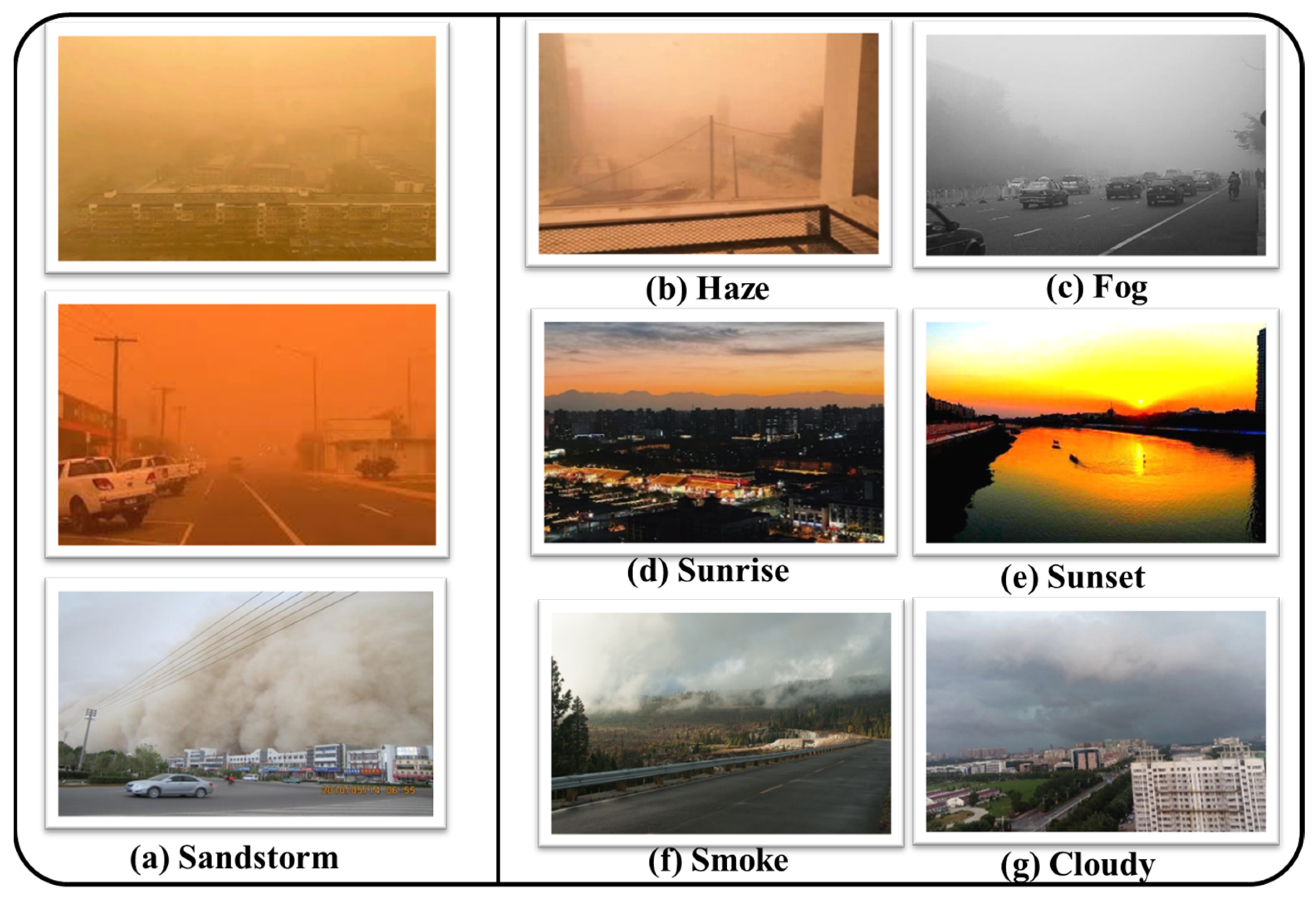
In meteorology, the definition of SDS weather levels is mainly based on horizontal visibility while referring to wind strength during SDS occurrences. A higher SDS level is associated with higher wind speed and lower visibility, and vice versa. It was observed that there were differences in the impact of different levels of SDS on surveillance images/videos.
For a lower-level SDS event, similar to fog, smog, and haze weather events, its appearance commonly causes a significant reduction in the sharpness and contrast of images captured by outdoor surveillance cameras, resulting in color shifting and missing detail problems [
14]. The degradation effect caused by these weather events can be generically expressed as follows [
10,
15,
16]:
where
is the observed intensity,
is the scene radiance,
is the global atmospheric light, and
is the medium transmission describing the portion of the light that is not scattered and reaches the surveillance camera.
Previous studies have pointed out that the radius of particles in SDSs is close to 25 µm, which is much larger than that in haze (0.01–1 µm) and fog (1–10 µm) conditions [
10,
17]. Since particles of different sizes show varying reflection interactions with visible light, the degradation effects of SDS and the other three weather conditions differ slightly. Nevertheless, the generic model (i.e., Equation (1)) still works, so images taken in these environments are hard to discriminate.
Visually, these weather events change the color of the surveillance image. Researchers were quick to build single or multiple color channels (classical ones like dark channels [
18]) that are sensitive to weather conditions, thus establishing a prior or assumption in terms of color space for fog, haze, smog, and SDS removal and image enhancement tasks. Single channels of RGB [
19,
20], HSV [
21], and YIQ [
22] color spaces are popular options. As shown in
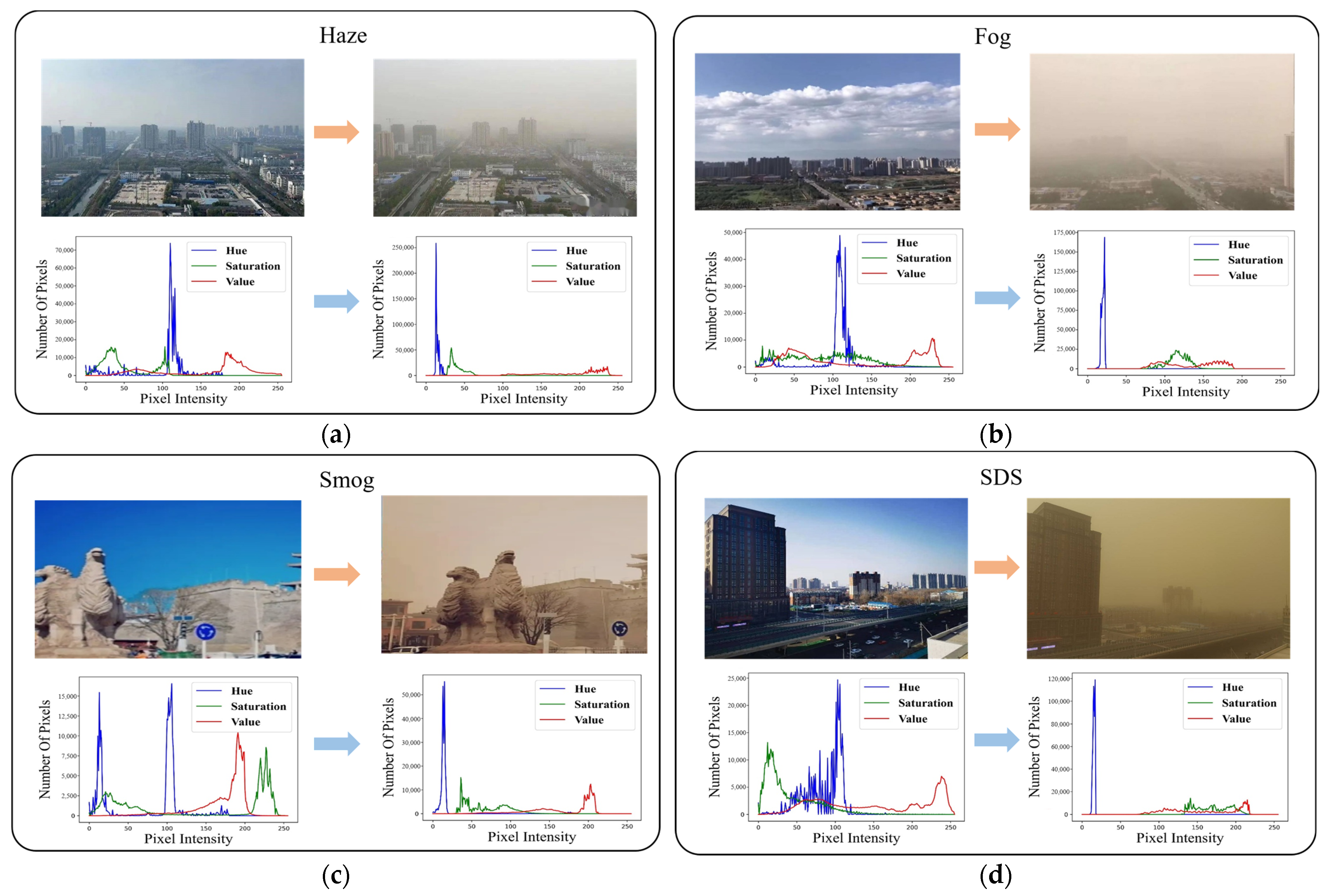
Figure 1, surveillance images captured under haze, fog, smog, and SDS weather conditions were randomly selected. Their effects on the surveillance images in HSV color space were compared.
Figure 1 illustrates that the listed weather events blurred the natural images. Moreover, the Hue color channel exhibits a single-peak pattern in the weather-influenced images and can be considered as a color prior or assumption of these blurred images. To date, image deblurring algorithms still favor this strategy highly and have made significant progress [
17,
19,
23,
24].
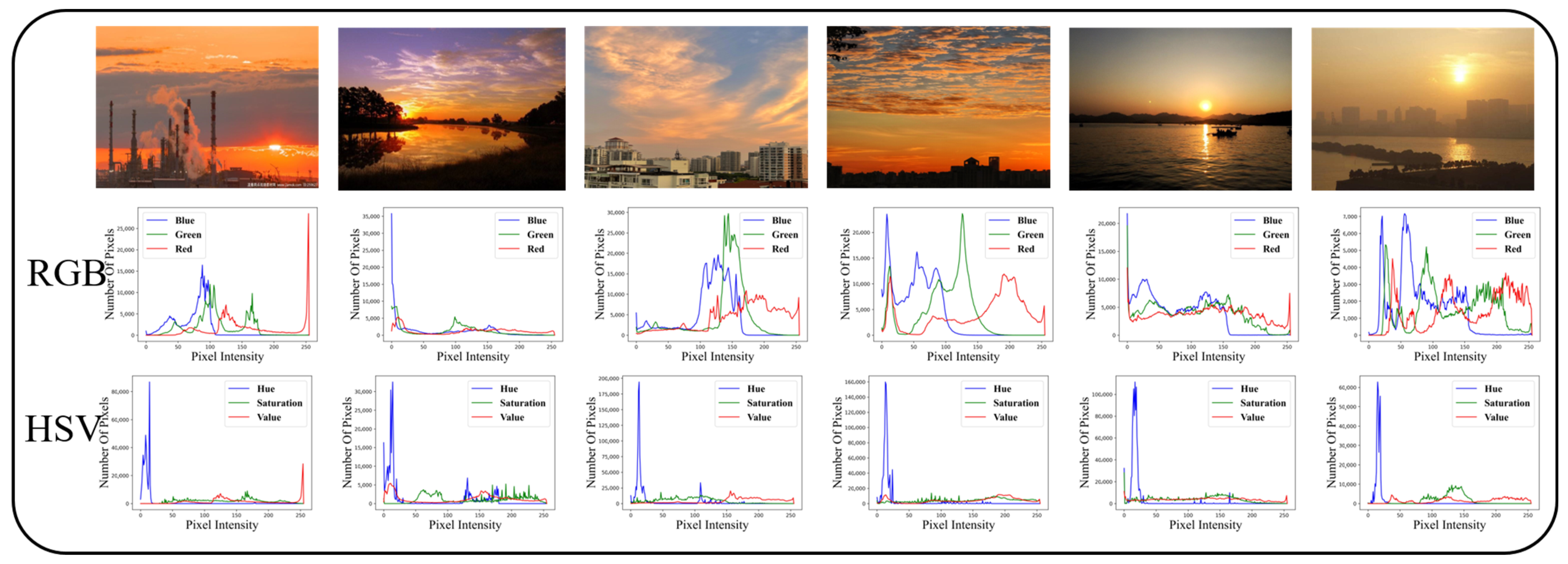
In addition to the images taken during the above weather, we found that similar surveillance images also have single peaks in the Hue channel, as shown in
Figure 2, making it more challenging to accurately distinguish SDSs in surveillance images.
Essentially, the purpose of the deblurring studies is to realize image restoration, which solves the problem of inconsistency between SDS images and the corresponding natural images. In contrast, our study focuses on monitoring the appearance of SDS via surveillance cameras. The crucial point is accurately distinguishing those surveillance scenarios that are similar to SDS. That is, sharing similar image characteristics with fog, haze, smog, etc., makes it more challenging to accurately distinguish SDS visually.
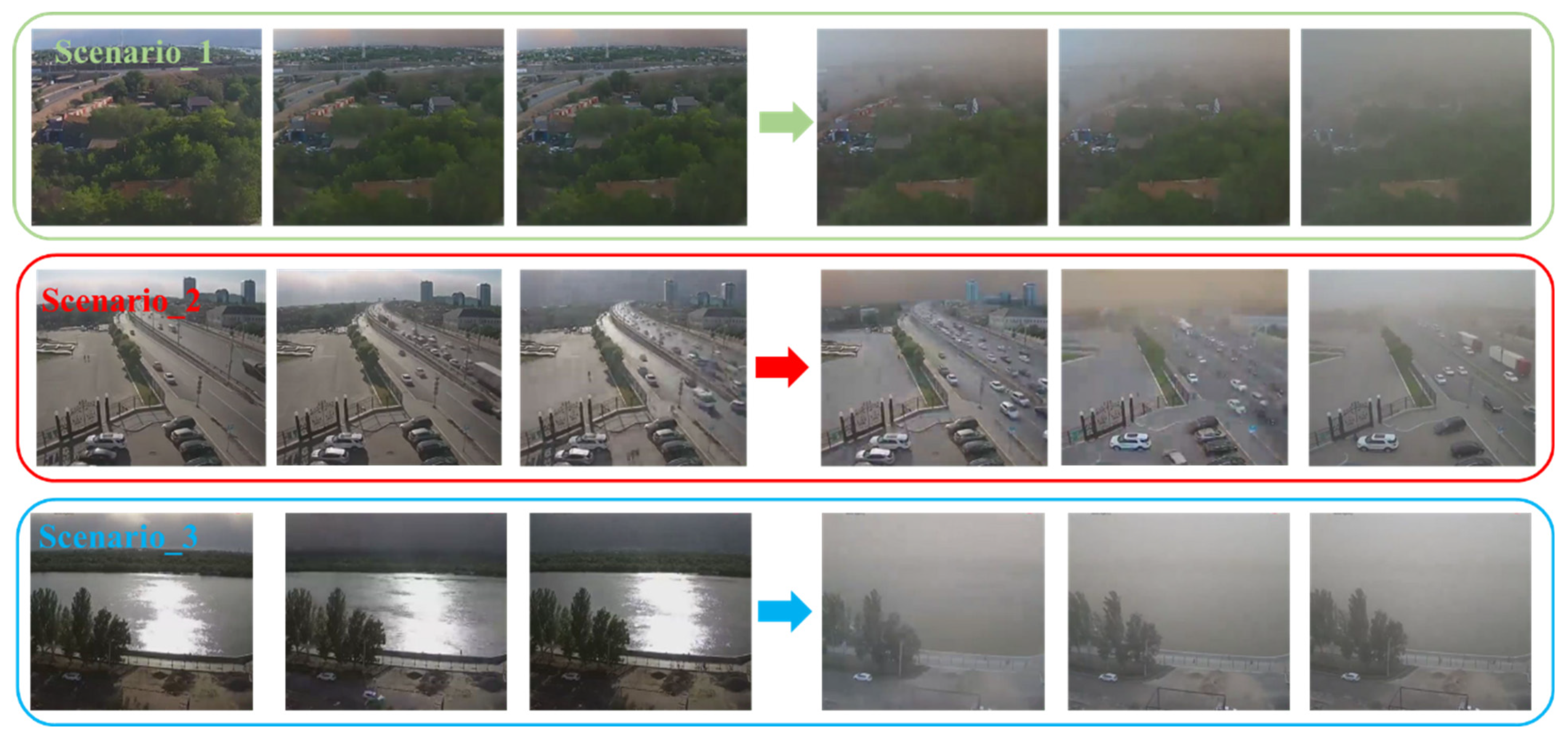
High-level SDS usually move fast together with low visibility. Here, a surveillance video recording the complete process of SDS from generation to transiting is collected, whose key frames are shown in
Figure 3. While still using the image HSV color space as an example, it can be observed that as the SDS moves and the proportion of sand in the image changes, accompanied by changes in the characteristics of the HSV color space (for example, in the first two images the single-peak pattern of the Hue channel is not apparent). Therefore, the image features of high-level SDS events are dynamically changing, resulting in the fixed manual image features needing to be more manageable to describe thoroughly the randomly occurring SDS events in nature.
Given the dynamic behavior of SDSs and the high similarity of image features with relevant scenarios, constructing image features based on specific channels for a robust and accurate description of SDSs poses significant challenges. Inspired by [
17], we consider the three channels (R, G, B) to be related and not independent. Therefore, taking the original image as an inseparable indivisibility in the form of a tensor for the input of the following detection algorithm.
2.2. Multi-Stream Attention-Aware CNN Network
As described in
Section 2.1, how to detect the occurrence of SDSs from surveillance images, mainly to distinguish SDS events from similar scenarios, becomes a fundamental problem for a detector to solve. With the development of deep learning technology, CNN-based algorithms have achieved satisfactory performance in object detection and classification tasks, bringing new opportunities to construct surveillance camera-based SDS detectors. On the other hand, inspired by the biological systems of humans that tend to focus on the distinctive parts when processing large amounts of information, the attention mechanism has the advantage of solving the problem of information overload and improving the accuracy of results [
25,
26]. As one of the latest advancements in deep learning, the attention mechanism has become an essential tool in deep learning [
27,
28].
In this section, the attention mechanism is employed to locate the most salient components of the feature maps in CNNs and to remove the redundancy. Then, a Multi-Stream Attention-aware CNN Network (MA-CNN) is proposed for SDS detection from surveillance images, as shown in
Figure 4. In MA-CNNs, the input data are simultaneously fed into multiple streams with different scales. In each stream, the features acquired by the stacked 2D CNN layers are fed into the spatial attention layer to acquire more focused SDS-sensitive features. Then the two layers are concatenated as input to a deeper layer.
Considering a CNN with
layers, the hidden state of layer
is represented as
, where
. In this notation, the input image can be defined as
. The convolutional layer consists of two parts learnable parameters, that is, the weight matrix
that connects layer
and layer
and the bias term vector
. Hence, each neuron in convolutional layer
is only connected with a local region on
and
is shared among all spatial locations. In order to improve translation invariance and representation capability, convolutional layers are interleaved with point-wise nonlinearity (i.e., Leaky ReLU, whose parameter alpha = 0.1 [
29]) and nonlinear down-sampling operation (i.e., 2D max pooling). The feature map of
can be obtained by the following:
where
denotes the 2D convolution operation.
As shown in
Figure 4, in order to enable the proposed network to learn richer semantic representations of the input image progressively, the number of channels in the outputs of successive blocks gradually increases as 64 → 128 → 256 → 512, and the kernel size of the connects layer gradually increases as 3 × 3 → 5 × 5 → 7 × 7. We integrate an attention mechanism [
30] into each stream. As described in
Section 3.1, considering the high similarity between SDSs and other monitoring scenarios (e.g., fog, smog, and haze), we introduce spatial attention mechanism to adaptively bootstrap features related to the key SDS-relevant features and pay less attention to those less feature-rich regions. The features obtained from the spatial attention layer and the last CNN layer are then concatenated as the final vectors of each stream. The details of the spatial attention mechanism are shown in
Figure 5.
For an input feature
with a size of
, firstly, the spatial information of a 2D feature map is generated by the average pooling feature (
) and max pooling feature (
), respectively. Then,
and
are concatenated and convolved by a standard convolution layer, producing a 2D spatial attention feature map
. The spatial attention is computed as follows:
where
denotes the sigmoid function and
means the convolution operation with the filter size of 7 × 7.
Moreover, to mitigate overfitting, the 0.5 via spatialdropout2D [
31] is added to each stream’s second and last layers. Then, the feature responses from three streams are concatenated and fed into a GlobalAveragePooling2D output layer to produce the final vectors. Lastly, a fully connected layer with a size of 512 and a Softmax classifier can be utilized for a two-class classification.


