Abstract
Synthetic aperture radar interferometry (InSAR) has emerged as an effective technique for monitoring potentially unstable landslides and has found widespread application. Nevertheless, in mountainous reservoir regions, the precision of time-series InSAR outcomes is often constrained by topography-dependent atmospheric delay (TDAD) effects. To address this limitation, we propose a novel InSAR time-series method that integrates TDAD correction. This approach employs advanced deep learning algorithms to individually model and mitigate TDAD for each interferogram, thereby enhancing the accuracy of small baseline subset InSAR (SBAS-InSAR) and stacking InSAR time-series analyses. Utilizing Sentinel-1 data, we apply this method to identify potential landslides in the Baihetan reservoir area, located in southwestern China, where we successfully identified 26 potential landslide sites. Comparative experimental results demonstrate a significant reduction (averaging 70% and reaching up to 90%) in phase standard deviation (StdDev) in the corrected interferograms, indicating a marked decrease in phase–topography correlation. Furthermore, the corrected time-series InSAR results effectively remove TDAD signals, leading to clearer displacement boundaries and a remarkable reduction in other spurious displacement signals. Overall, this method efficiently addresses TDAD in time-series InSAR, enabling precise identification of potentially unstable landslides influenced by TDAD, and providing essential technical support for early landslide hazard detection using time-series InSAR.
1. Introduction
Landslide disasters represent a significant threat in high mountainous and canyon regions across the globe, resulting in thousands of injuries, fatalities, and substantial damage to critical infrastructure [1]. The southwestern region of China is particularly susceptible to frequent landslides due to its intricate terrain and diverse geological structures, which pose significant societal and economic risks. Early identification of landslide hazards becomes imperative to mitigate casualties and avert losses resulting from such disasters.
In recent decades, synthetic aperture radar (SAR) interferometry (InSAR) technology has been widely applied in landslide monitoring due to its all-weather, all-day coverage capabilities, among other advantages [1,2,3,4,5,6,7,8,9,10,11,12,13]. Researchers have extensively utilized time-series InSAR techniques to identify potential landslide hazards [5,6,14,15,16,17,18,19,20]. Time-series InSAR techniques are still limited by atmospheric delays [21,22,23,24,25,26,27,28,29], although many methods have been proposed to correct different atmospheric delays to improve the accuracy of displacement monitoring (e.g., [27,28,30,31,32]). Among these atmospheric delays, the influence of topography-dependent atmospheric delay (TDAD) is particularly severe in many cases. This component is caused by variations in atmospheric refractivity in the vertical profile and it is highly correlated with the topography and primarily affects areas with significant terrain variations [33]. Numerous methods have been proposed to correct TDAD in InSAR, which can be broadly categorized into three types. The first type is the mathematical modeling method, where TDAD is estimated based on the phase data themselves. The most widely used method assumes a linear relationship between the interferometric phase and topography to estimate the TDAD [4,34]. The second type uses external auxiliary data to estimate TDAD, including meteorological models [34,35], GNSS data [36,37,38,39,40,41,42], spectral measurements [43,44], or a fusion of these data sources [1,45]. The third type is based on deep neural network approaches, such as [46,47]; methods of this kind are based on the premise that topography is strongly correlated with TDAD and aim to model it to reduce the influence of TDAD. Although the above methods have achieved certain results in different regions, there are some drawbacks to them. The first type, mathematical modeling, estimates the TDAD based on a certain model for all the interferograms of all conditions. It is clear that even in the same area, the interferograms with different SAR acquisitions affected by the TDAD are not the same [4,48]. The second type requires external data, which are constrained by low spatiotemporal resolution [1,23,49], and the third type, based on deep learning, has demonstrated successful TDAD correction in individual interferograms. However, currently, there is a lack of relevant cases and analysis regarding the improvement of time-series InSAR results influenced by TDAD, which deserves further research.
In this study, we propose a time-series InSAR method that incorporates TDAD correction using a deep neural network to enhance the accuracy of the interferometric phase in each interferogram. The corrected interferograms are then utilized in small baseline subset InSAR [50] (SBAS-InSAR) and stacking InSAR [51] time-series techniques. We apply this method to identify potential landslide hazards in the Baihetan reservoir area of southwestern China using Sentinel-1 data. The effectiveness and applicability of the proposed method in TDAD correction are evaluated from both qualitative and quantitative perspectives. The improved time-series InSAR algorithm can significantly reduce the influence of TDAD, enhance the reliability of time-series results, identify landslides affected by TDAD, and is of great significance for the early identification and monitoring of potential landslides.
2. Study Area and Datasets
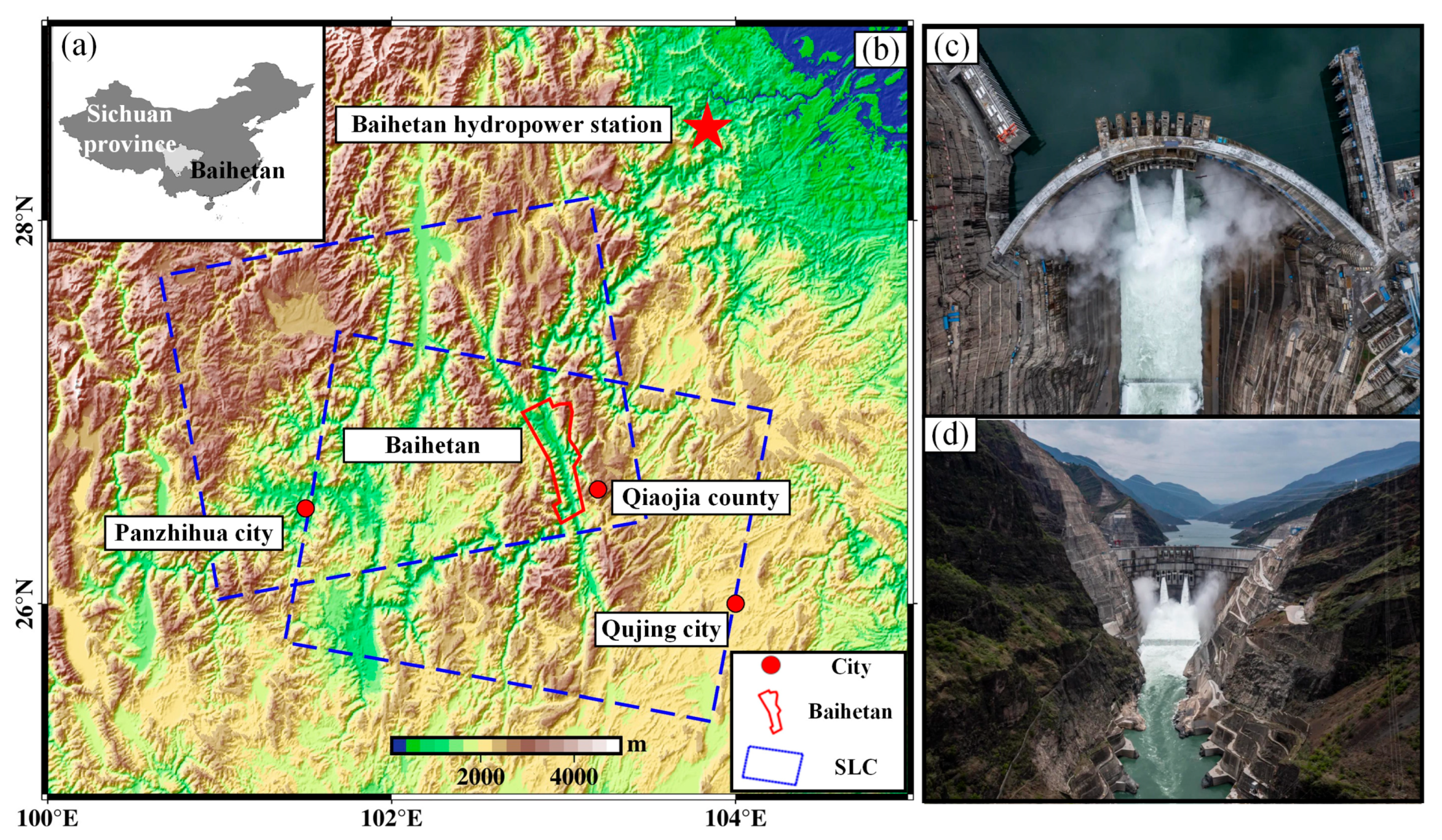
As shown in Figure 1, the Baihetan hydropower station is located in the territory of Ningnan County, Sichuan Province, and Qiaojia County, Yunnan Province, downstream of the Jinsha River. It is the second cascade power station in the downstream mainstream of the Jinsha River, mainly for power generation, with additional functions of flood control, sediment interception, improvement of downstream navigation conditions, and development of the reservoir area for navigation purposes. The region is situated on the southeastern edge of the Qinghai–Tibet Plateau, with elevations ranging from 1000 to 3000 m. It belongs to the high mountains and plateau geomorphic unit of southwestern Sichuan and northeastern Yunnan, as well as the Transverse Mountain System. The area is primarily composed of fluvial erosion landforms, tectonic landforms, and glacial erosion landforms, with deep-cut valleys and significant weathering and erosion. This study focuses on the area of approximately 800 km² along the main channel of the Jinsha River, from Hulukou to Xiangbilin, where the Baihetan Hydropower Station is situated. The study area is densely populated, with residential areas along the river, multiple transportation routes, and intense human engineering activities. The area is characterized by poor stability, large elevation differences in slope, and sparse vegetation. Additionally, factors such as river erosion make it highly susceptible to geological hazards such as landslides, collapses, and debris flows. Therefore, it is a key section for geological hazard prevention and control in the Baihetan reservoir area.
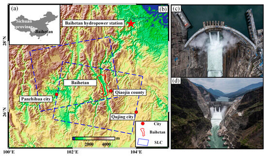
Figure 1.
(a) The location of Baihetan; (b) topographic map of the study area; (c,d) photos of Baihetan hydropower station [16].
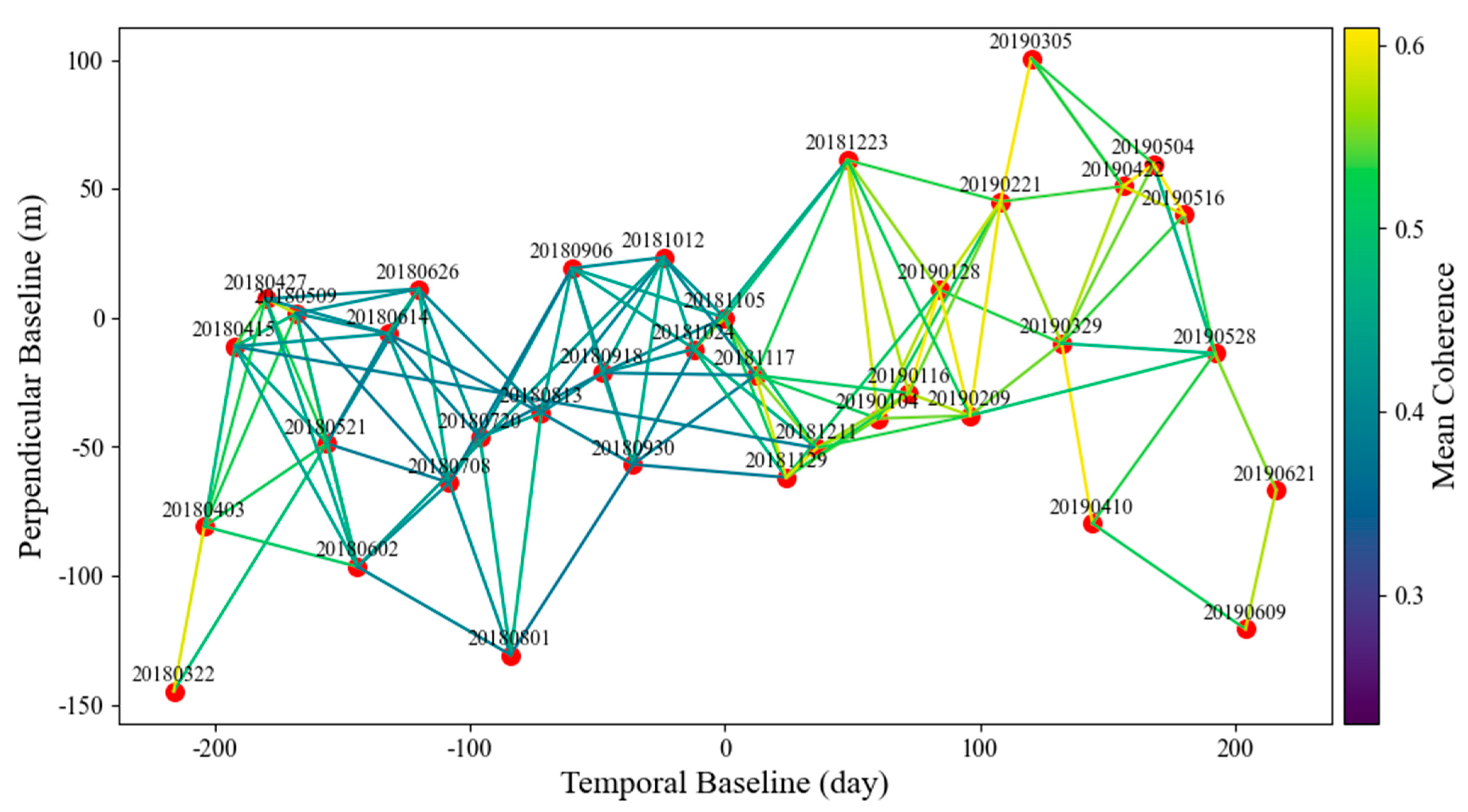
This study utilizes Sentinel-1 SAR data for InSAR time-series analysis. The satellite data are acquired in the C-band with short revisit periods and wide coverage, and are widely applied in geological hazard monitoring. A total of 37 descending single-look complex (SLC) images were acquired for the study area (Figure 2) for the period from March 2017 to June 2018. The SLC images were obtained in VV polarization mode under the interferometric wide swath mode, with an incidence angle of 39.99°.

Figure 2.
Temporal and spatial baseline map. The color bar represents the coherence of interferometric pairs.
3. Methodology
3.1. Typical Time-Series InSAR Method Used in This Study
Differential stacking [51], based on D-InSAR technology, is a form of InSAR technique that involves the superimposition and weighted averaging of multiple-phase images generated through D-InSAR processing. Its primary objective is to reduce errors and obtain more precise surface displacement information. This method assumes that the noise phase in the interferograms is random and equal and that the surface within the region exhibits linear changes. Based on this assumption, it effectively reduces the generation of random errors. The main steps involve the selection of suitable interferometric pairs and the subsequent stacking of all interferometric images, weighted by time baseline. This process ultimately yields a displacement quantity that is accumulated based on time baselines. Consequently, in the final phase image, the quality of results is enhanced, resulting in more accurate displacement information.
PS-InSAR [52] (persistent scatterer interferometric synthetic aperture radar) technology generates interferometric pairs, and due to the selection of a single master image, it may include interferometric pairs with longer spatial baselines, making it susceptible to spatial decorrelation effects. SBAS (small baseline subset) technology, proposed by Berardino et al. [50] in 2002, is a technique that reduces the effects of temporal and spatial decorrelation and atmospheric delays in traditional InSAR techniques. The basic principle is to partition existing images into subsets by setting time and spatial baseline thresholds. This ensures that the images within a subset have small inter-image baselines, while the baselines between subsets are large. The least squares method is used to compute the subsidence sequence within each subset, and a singular value decomposition (SVD) method is employed to jointly solve all subsets, thereby obtaining the complete subsidence sequence over the entire period.
3.2. Time-Series InSAR with TDAD Deep Learning Correction
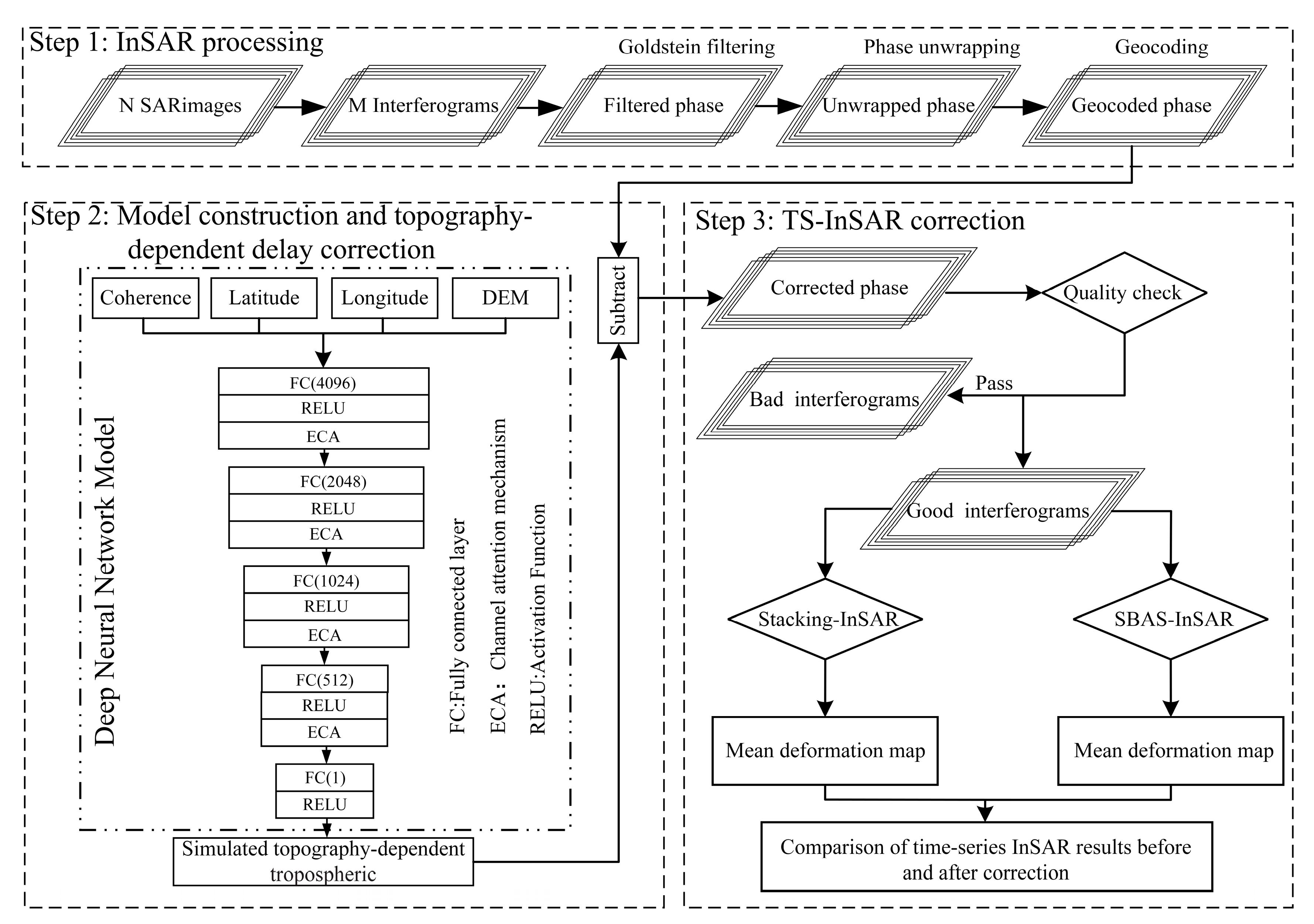
This paper takes into account the topography and displacement characteristics of the Baihetan area, as well as the ability of neural networks to approximate any function model, as indicated by the universal approximation theorem [53]. Therefore, we employ a neural network model to correct TDAD and obtain more reliable time-series InSAR results. The specific implementation process is outlined in Figure 3.
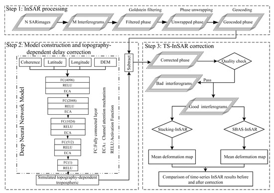
Figure 3.
Temporal–spatial InSAR technique integrated with a TDAD correction process.
Firstly, SAR data preprocessing is conducted, involving processing N scenes of SLC images to obtain M pairs of differential interferometric phases. The main operations include registration, interferometry, filtering, phase unwrapping, and geocoding. After obtaining M pairs of differential interferometric results, considering the topography and displacement characteristics of the Baihetan reservoir area, a deep neural network model is constructed to model TDAD. The design of the deep neural network model is based on several aspects. Firstly, the characteristics of the problem to be solved are considered: (1) TDAD is related to topography, so the topography information is incorporated into the model during the modeling process; (2) long-scale delay signals often exist in the interferometric phase, so spatial location information, i.e., latitude and longitude information, needs to be considered during modeling; (3) due to the presence of decorrelation noise, the model needs to take into account the impact of noise signals. Thus, coherence data are integrated into the model. Furthermore, since different regions may have different dominant phase components (such as TDAD phase, long-scale dominant phase, etc. [47]), a channel attention mechanism module [54] is introduced in this study to address this issue. Moreover, considering the problem of underfitting and overfitting [55,56,57], appropriate network layer settings are needed. First, since the relationship between TDAD and topography is nonlinear and spatially heterogeneous, a sufficiently deep network layer is required to capture this complexity. Then, due to the limited extent of the Baihetan reservoir area, when the model is set to be too complex, its complexity may exceed the complexity of the problem. Taking these two points into consideration, this study sets the model layers to be 4096, 2048, 1024, 512, and 1. In addition, the main hyperparameter settings for training are as follows: A batch size of 8192 was used. The optimizer employed was adaptive moment estimation (Adam) [58], a widely adopted optimization algorithm in deep learning known for its merits of requiring fewer hyperparameters and delivering strong performance. The learning rate was set at 0.0002. The proposed neural network underwent 50 epochs of training. The loss function chosen was the mean squared error (MSE). The specific modeling process is as follows (1)–(9):
Once the model construction is completed, each pair of geocoded unwrapped phases along with their corresponding elevation, latitude, longitude, and coherence data are input into the deep neural network to perform TDAD correction for each interferometric pair. After obtaining the simulated TDAD phase, it is subtracted from the original phase to obtain the corrected unwrapped phase. Finally, the corrected unwrapped phase is used for time-series analysis (i.e., stacking InSAR and SBAS-InSAR) to obtain time-series results, and a comparison is made between the pre- and post-correction time-series results to analyze the performance.
4. Results and Discussion
4.1. Corrected Time-Series Results and Verification
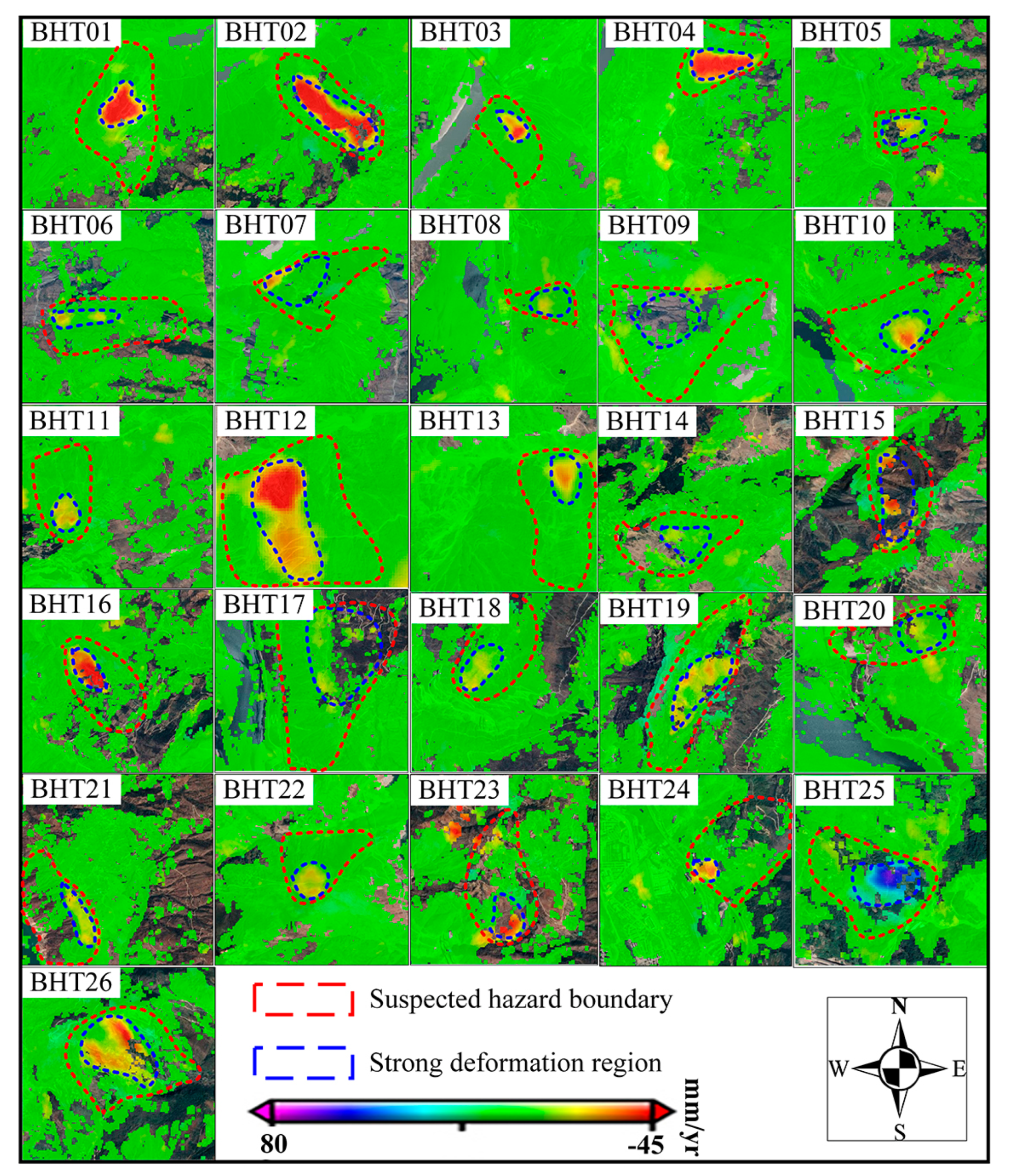
This paper presents a statistical analysis of the results of the time-series InSAR technique with TDAD correction for the Hulukou to Xiangbiling section in the Baihetan reservoir area, focusing on the identification of potential landslide hazards. Figure 4 illustrates the time-series InSAR displacement results in the Baihetan region after TDAD correction. Based on the InSAR displacement results corrected by the deep neural network, we successfully identified 26 potential landslide hazard points with significant displacement. All these potential landslides were validated by the optical remote sensing images and the local microtopography. After correcting TDAD, the InSAR technique demonstrates good reliability in high-precision time-series computation. Therefore, the landslides identified by InSAR exhibit high coherence and clear displacement, providing highly reliable monitoring results.
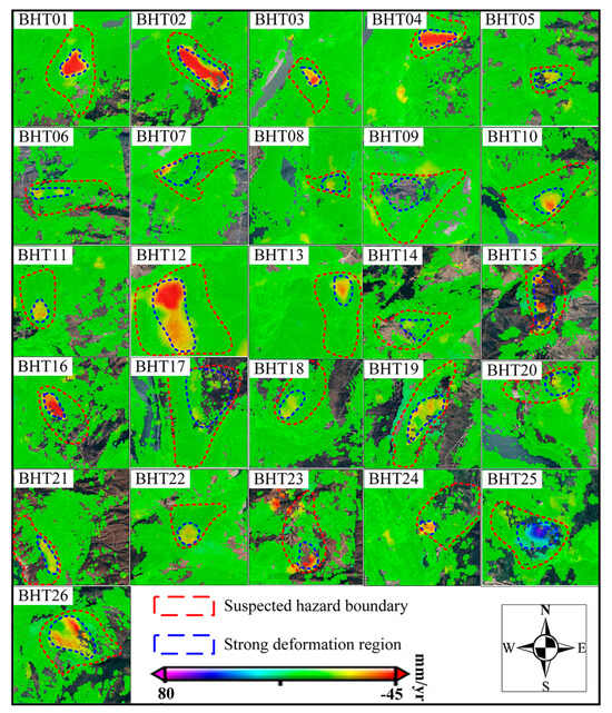
Figure 4.
Details of the results of the identification of suspected geologic hazard sites. The color bar represents the range of displacement.
In terms of the overall distribution, the potential landslide hazard points are distributed with 9 points on the left bank and 17 points on the right bank of the Jinsha River (Figure 4). Among these, nine points exhibit significant displacements, and three of them are shown corresponding to Google Earth images in Figure 5b–d.
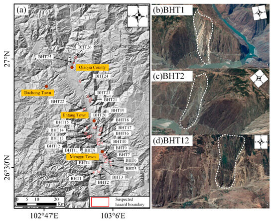
Figure 5.
(a) InSAR identification of geohazard hazard site distribution; (b–d) the typical slope Google Earth images.
4.2. Comparative Analysis of Results before and after Correction
4.2.1. Comparison and Analysis of the Interference Phase before and after Correction
To evaluate the effectiveness of the model, we selected two typical interferograms from the Baihetan reservoir area for analysis. Figure 6 shows the correction results for these two interferograms, with the first three columns presenting the original interferogram, simulated interferogram, and corrected interferogram, respectively. It is evident from the figures that the selected interferograms exhibit a correlation with topography and are significantly affected by TDAD (Figure 6a,d), highlighting the necessity of TDAD correction. Comparing the original interferogram and the simulated interferogram (Figure 6a,b,d,e), we can observe a high degree of spatial similarity between them. This indicates that the model successfully captured the TDAD in the interferograms. After model correction (Figure 6c,f), the phase becomes smoother overall, and its spatial correlation with topography is significantly reduced. This suggests that the model effectively learned and mitigated the TDAD characteristics, resulting in a more reliable and accurate corrected phase, which benefits the generation of more reliable time-series InSAR results.
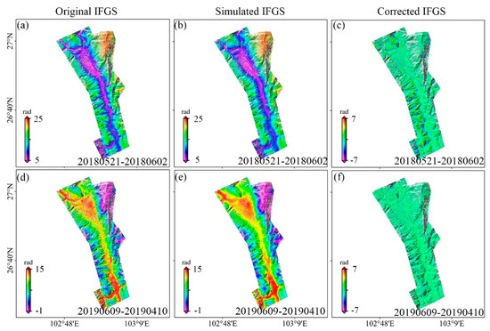
Figure 6.
Typical interferometric phase correction results in the Baihetan area. (a,d) The original interferometric phase; (b,e) the model-simulated interferometric phase; (c,f) the corrected interferometric phase. The color bar represents the differential phases.
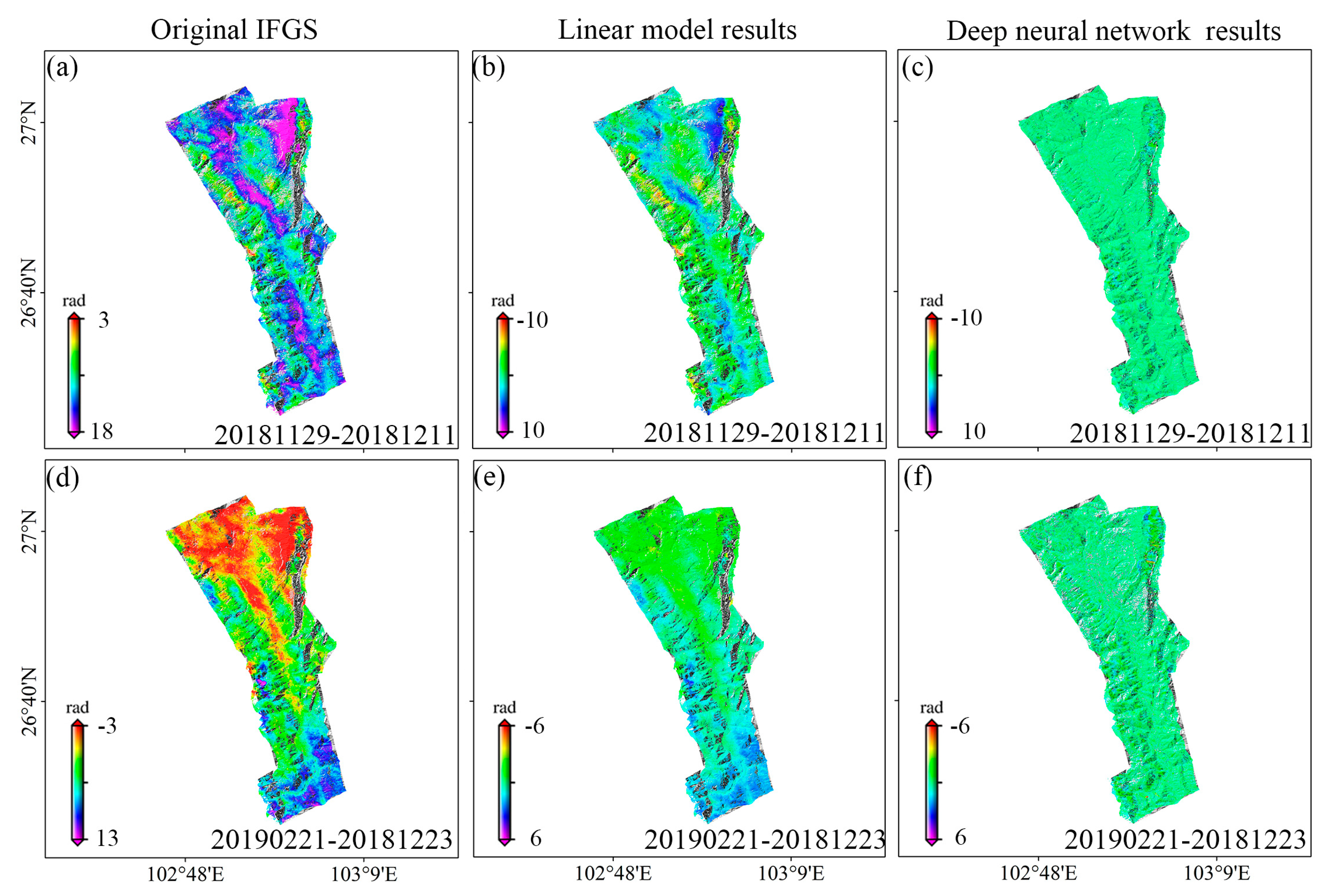
To validate the correction results of our method, we conducted a comparison with a traditional linear model atmospheric correction method. As shown in Figure 7, we present the results of the linear model and our deep neural network model corrections for two typical interferometric pairs in the Baihetan area. It is evident that after linear model correction, good correction results were obtained for some regions (Figure 7b,d) but the improvement is limited due to the spatial heterogeneity in atmospheric delay, which cannot be addressed using a specific model-based correction method [4,24,31], while clear global improvement was achieved (Figure 7c,f).
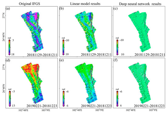
Figure 7.
Typical interferometric phase correction results in the Baihetan area. (a,d) The original interferometric phase; (b,e) linear-model-corrected interferometric phase; (c,f) deep-neural-network-corrected interferometric phase. The color bar represents the differential phases.
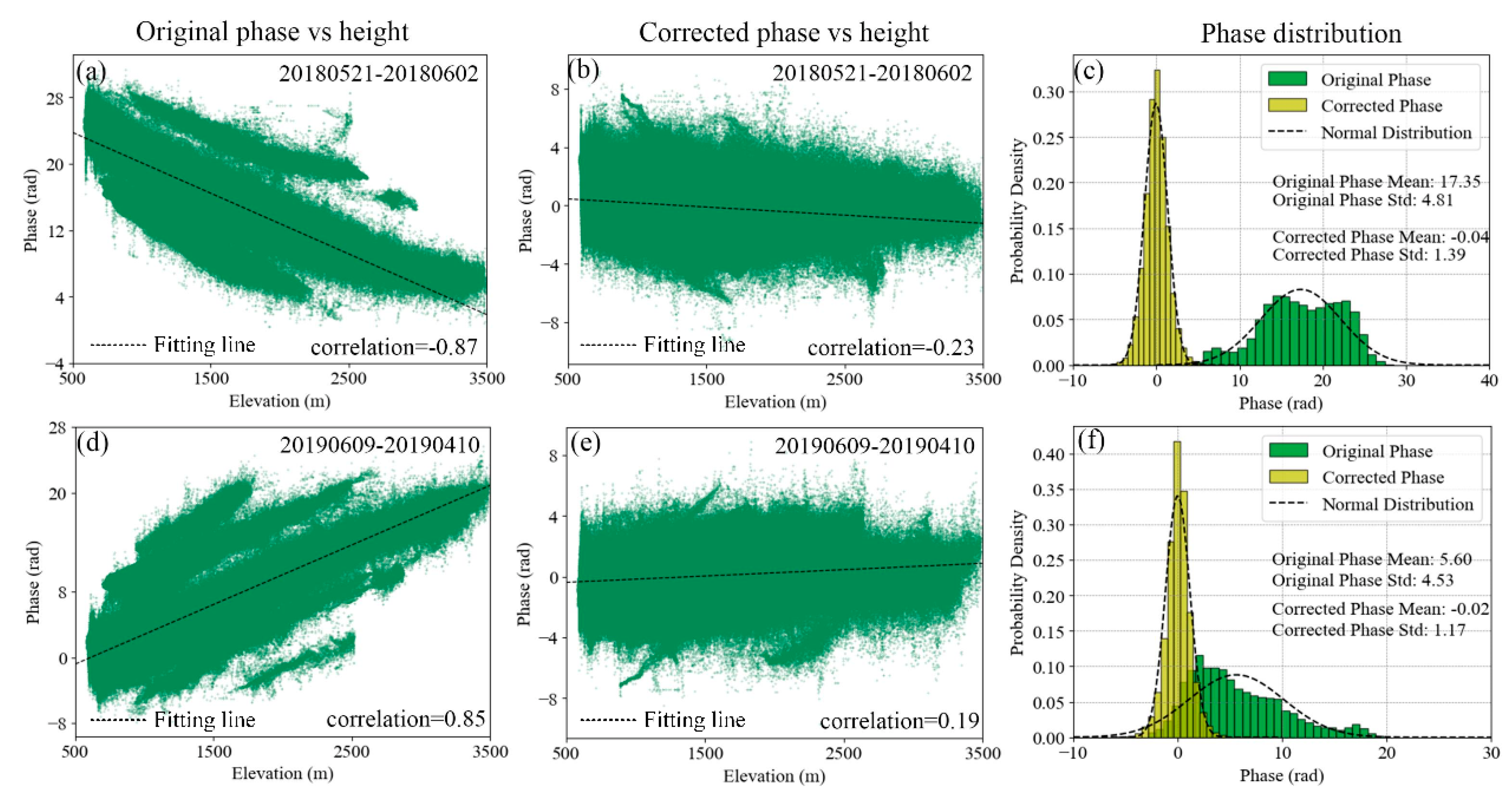
Furthermore, we conducted quantitative evaluations for the two typical interferograms in the Baihetan reservoir area (Figure 8). The evaluation includes the correlation between the phase and topography before and after correction and the distribution of the phase before and after correction.
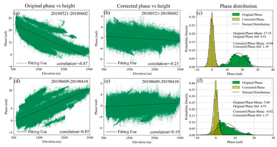
Figure 8.
Statistics of before and after correction of typical interferometric phases in the Baihetan area. (a,d) Phase and topography correlation before correction; (b,e) phase and topography correlation after correction; (c,f) phase distribution before and after correction.
In the first column, we calculated the correlation between the phase and topography before correction, and in the second column, we calculated the correlation after correction. The third column presents the distribution of the phase before and after correction. As the displacement phase is usually unrelated to topography, a reduced correlation between phase and topography indicates the successful removal of the TDAD. Figure 8a,d show that the original interferograms exhibit strong correlations with topography, with Pearson correlation coefficients of −0.87 and 0.85, respectively. After model correction, the correlation between topography and phase is significantly reduced, with Pearson correlation coefficients dropping to −0.23 and 0.19, respectively, representing an average reduction of 76% (Figure 8a–e). Moreover, after correction, the phase distribution becomes more concentrated, with its mean centered around zero, and the standard deviation (StdDev) significantly decreases from 4.81 and 4.74 to 1.39 and 1.17, representing an average reduction of 73% (Figure 8c,f).
In summary, through qualitative and quantitative evaluations of the two typical interferograms from the Baihetan reservoir area, we verified the effectiveness of the model correction. The correlation between phase and topography is significantly reduced after correction, and the phase distribution becomes more concentrated with reduced StdDev. These results indicate that the model successfully removes TDAD, thereby enhancing the reliability of the phase results and contributing to generating more reliable time-series InSAR results.
To assess the applicability of the model, we conducted a StdDev statistical analysis on all interferograms from the Baihetan reservoir area. The specific results are shown in Figure 9. Figure 9a illustrates the percentage of reduction in phase StdDev for the selected 127 differential interferograms, while Figure 9b represents the corresponding distribution.
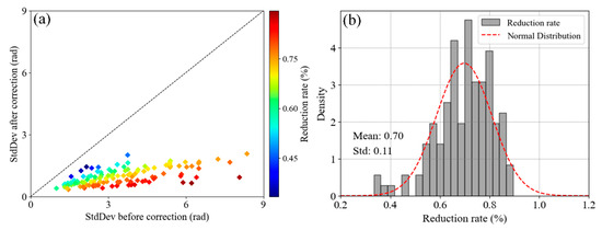
Figure 9.
Statistics of phase StdDev before and after correction of all interferometric phases in the Baihetan area. (a) The result of the proportion of phase StdDev reduction for all interferometric phases; (b) the distribution of the proportion of StdDev reduction.
From Figure 9a, it is evident that after correction, the StdDev of all interferograms significantly decreases, indicating the model’s excellent TDAD correction performance. However, it is essential to note that if the model lacks robustness or applicability, there might be substantial differences in the correction effects for different interferograms or regions. Therefore, when the StdDev of the percentage reduction in the interferogram StdDev is low, it indicates that the model exhibits good robustness and applicability. Figure 9b presents the distribution of the percentage reduction in interferogram StdDev. The results show that the mean percentage reduction is 0.70, with a StdDev of 0.11. This indicates that the model demonstrates excellent robustness and wide applicability, making it effectively suitable for TDAD correction.
4.2.2. Comparison and Analysis of Time-Series Results before and after Correction
As shown in Figure 10 and Figure 11, this study utilized two time-series InSAR techniques to calculate the annual average displacement rates in the Baihetan reservoir area. Figure 10A and Figure 11A show the displacement results before correction, while Figure 10B and Figure 11B show the displacement results after correction.
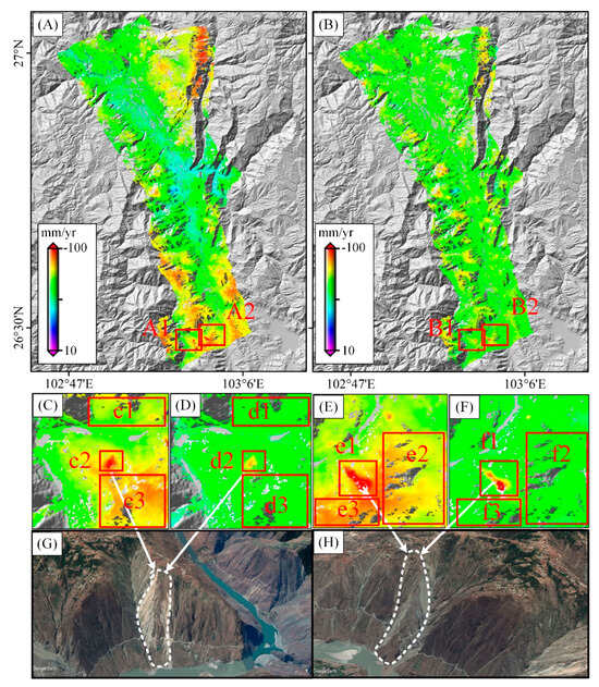
Figure 10.
TDAD correction using the stacking InSAR technique in the Baihetan area. (A,B) The stacking InSAR result before/after correction; (C,D) the details of area A1 before/after correction; (E,F) the details of area A2 before/after correction; (G,H) the corresponding Google image maps. The color bar represents the range of displacement.
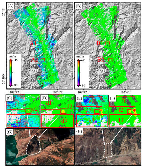
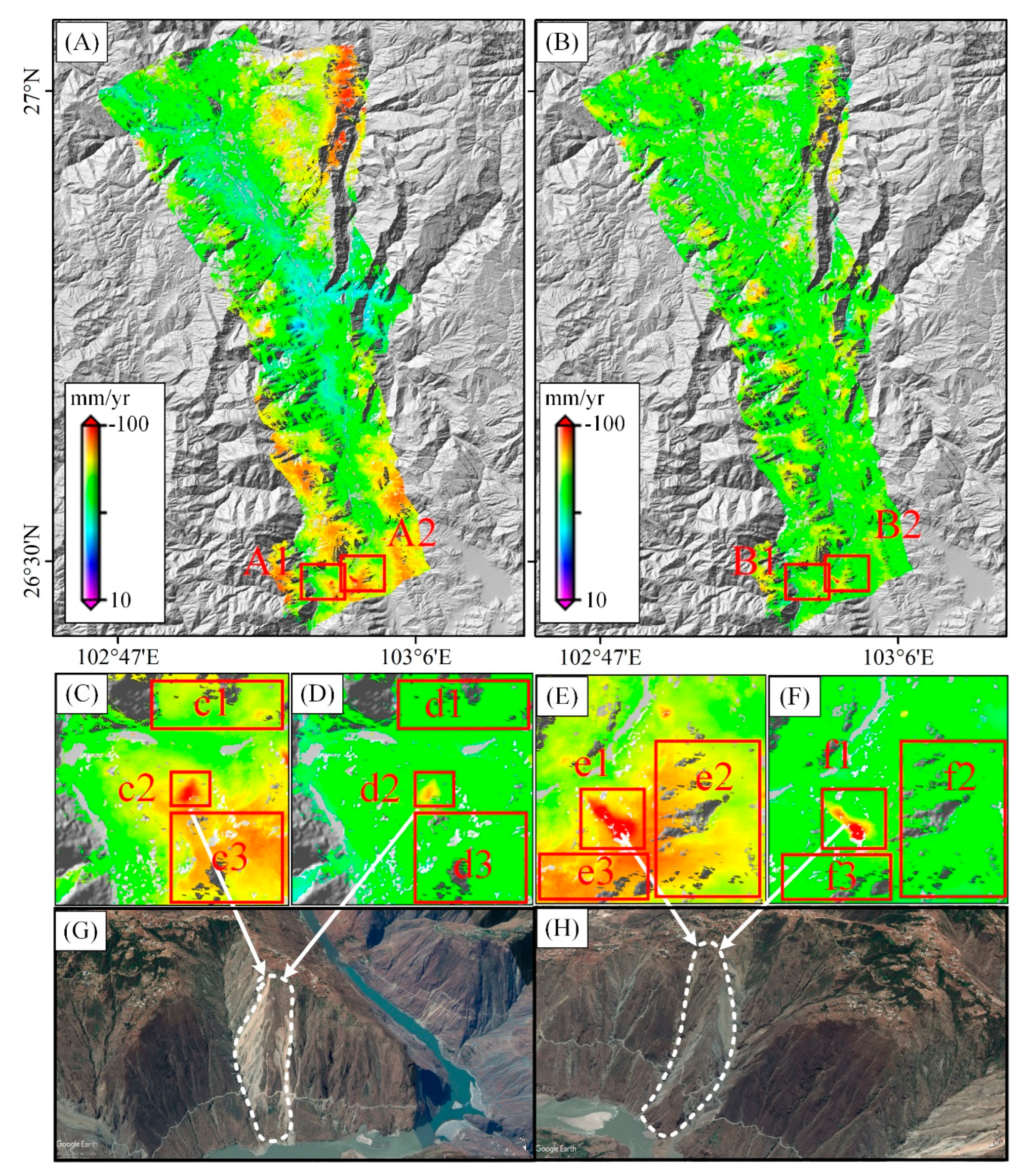
Figure 11.
TDAD correction using the SBAS-InSAR technique in the Baihetan area. (A,B) The SBAS-InSAR result before/after correction; (C,D) the details of area A1 before/after correction; (E,F) the details of area A2 before/after correction; (G,H) the corresponding Google image maps. The color bar represents the range of displacement.
Firstly, a comparative analysis was conducted on the stacking InSAR TDAD corrected results in the Baihetan area. From Figure 10A, it can be observed that although phase stacking can effectively reduce random noise in the interferograms and estimate average displacement rates, the TDAD signals in the interferograms, which are non-stationary over large spatial scales, cannot be simply removed through phase stacking, leading to the presence of systematic errors in the results. Conversely, after TDAD correction, most of the systematic errors are eliminated, leaving only local small-scale residual signals (Figure 10B).
We selected two representative areas to show the performance of TDAD correction in the stacking InSAR results. As shown in Figure 10C,E, the displacement center was affected by TDAD, and this signal covered the entire region, resulting in an overestimation of the displacement results, causing unclear displacement boundaries, and thus making it difficult to accurately locate displacement boundaries (Figure 10(c2,e1)). After correction (Figure 10B), the TDAD signal was effectively removed, and the landslide boundaries appeared more distinct and accurate (Figure 10(d2,f1)). Therefore, it is concluded that the time-series InSAR results after TDAD correction can accurately characterize surface displacements, which is of great significance for the early identification of landslide hazards in the Baihetan area.
Next, the analysis was extended to the displacement results of SBAS-InSAR. As shown in Figure 11 A, in the original displacement results, long-wavelength signals did not dominate, but there existed spatially distributed signals related to topography, i.e., TDAD signals. In this case, the non-stationarity of the atmospheric delay signals in the interferograms was mainly caused by TDAD. As mentioned in Section 3, the deep neural network effectively reduces the errors caused by TDAD noise. Comparing Figure 11A and B, it can be observed that after TDAD correction, the local-topography-dependent component was effectively removed.
We selected two representative areas to show the performance of TDAD correction in the SBAS-InSAR results. From Figure 11(c1,c3,d1,d3), it is evident that within a small range, the time-series results were influenced by TDAD, resulting in overall accelerated displacement results. Based on the previous analysis of c1 and d3 (potential landslide hazard areas), it can be observed that after correction, the values in the displacement area were overestimated, and the contours became more evident. The main reason was the existence of error signals, causing an overall overestimation in that region while relatively reducing the values in the displacement area, thus disrupting the displacement contours. Consequently, the area was not identified in the pre-correction time-series results. Similar analyses apply to E(e1–e3) and F(f1–f3), and are thus not repeated here.
In conclusion, through the comparative analysis of the displacement results in SBAS-InSAR, it was found that the DNN effectively removes the TDAD signal and can identify potential landslide hazard points after TDAD correction.
5. Conclusions
This study focuses on the correction of TDAD in time-series InSAR for potential landslide identification and monitoring. We present a novel time-series InSAR algorithm based on deep learning for correcting TDAD. We used Sentinel-1 image data from 2018 to 2019 and applied the proposed method to identify the potential landslide hazards in the Baihetan reservoir area. A comparative analysis was conducted between the time-series results obtained using the new algorithm and original time-series methods. Our major findings can be summarized as follows:
1. Comparing the results of interferometric pairs considering TDAD effects, the StdDev of the interferometric phases was reduced by an average of 70% and up to 90% among 127 interferograms in the study area. The proposed method was compared with traditional approaches (GACOS), demonstrating the superiority of TDAD correction. The proposed method demonstrates certain applicability, with a StdDev of the StdDev reduction ratio being only 0.11.
2. The comparison of the time-series InSAR results before and after TDAD correction reveals that the corrected time-series displacement results show clearer displacement boundaries and can identify potential landslide hazards affected by TDAD signals. This finding is of significant importance for the early identification and warning of potentially unstable landslides.
3. The improved time-series InSAR results successfully identified 26 potential landslide hazard points in the Baihetan area. This finding provides robust support for early identification and warning of landslides, making it highly valuable for mitigating and responding to potential geological disasters.
Author Contributions
All the authors participated in editing and reviewing the manuscript. Conceptualization, validation, supervision, K.D.; methodology, software, data analysis, validation, H.Z.; conceptualization, validation, supervision, J.X. conceptualization, supervision, X.T. validation, M.W. writing—review, R.L. writing—editing, Y.P. validation, Z.L. All authors have read and agreed to the published version of the manuscript.
Funding
This research is funded by the National Key Research and Development Program of China (grant no. 2021YFB3901403), National Natural Science Foundation of China (Grant No. 42371462), the Sichuan Province Science Fund for Distinguished Young Scholars (2023NSFSC1909), the China Postdoctoral Science Foundation fellowship (grant no. 2020M673322), the State Key Laboratory of Geohazard Prevention and Geoenvironment Protection Independent Research Project (grant no. SKLGP2020Z012), and the Open Research Fund Program of the MNR Key Laboratory for Geo-Environmental Monitoring of the Great Bay Area: 20220006.
Data Availability Statement
The Sentinel-1 dataset was provided by the European Space Agency (ESA), through the Alaska Satellite Facility (https://vertex.daac.asf.alaska.edu/).
Acknowledgments
We thank ESA for the Sentinel-1A satellite data and corresponding precision orbital data, Partial figures in this paper were made with General Mapping Tools software (http://gmt.soest.hawaii.edu/). We also thank the University of Newcastle for providing data on tropospheric correction data through GACOS (2019) (http://www.gacos.net/).
Conflicts of Interest
The authors declare no conflict of interest.
References
- Dong, J.; Zhang, L.; Liao, M.; Gong, J. Improved Correction of Seasonal Tropospheric Delay in InSAR Observations for Landslide Deformation Monitoring. Remote Sens. Environ. 2019, 233, 111370. [Google Scholar] [CrossRef]
- Del Soldato, M.; Solari, L.; Poggi, F.; Raspini, F.; Tomás, R.; Fanti, R.; Casagli, N. Landslide-Induced Damage Probability Estimation Coupling InSAR and Field Survey Data by Fragility Curves. Remote Sens. 2019, 11, 1486. [Google Scholar] [CrossRef]
- Dai, K.; Li, Z.; Tomás, R.; Liu, G.; Yu, B.; Wang, X.; Cheng, H.; Chen, J.; Stockamp, J. Monitoring Activity at the Daguangbao Mega-Landslide (China) Using Sentinel-1 TOPS Time Series Interferometry. Remote Sens. Environ. 2016, 186, 501–513. [Google Scholar] [CrossRef]
- Wang, Y.; Dong, J.; Zhang, L.; Zhang, L.; Deng, S.; Zhang, G.; Liao, M.; Gong, J. Refined InSAR Tropospheric Delay Correction for Wide-Area Landslide Identification and Monitoring. Remote Sens. Environ. 2022, 275, 113013. [Google Scholar] [CrossRef]
- Dai, K.; Deng, J.; Xu, Q.; Li, Z.; Shi, X.; Hancock, C.; Wen, N.; Zhang, L.; Zhuo, G. Interpretation and Sensitivity Analysis of the InSAR Line of Sight Displacements in Landslide Measurements. GISci. Remote Sens. 2022, 59, 1226–1242. [Google Scholar] [CrossRef]
- Roy, P.; Martha, T.R.; Khanna, K.; Jain, N.; Kumar, K.V. Time and Path Prediction of Landslides Using InSAR and Flow Model. Remote Sens. Environ. 2022, 271, 112899. [Google Scholar] [CrossRef]
- Crippa, C.; Valbuzzi, E.; Frattini, P.; Crosta, G.B.; Spreafico, M.C.; Agliardi, F. Semi-Automated Regional Classification of the Style of Activity of Slow Rock-Slope Deformations Using PS InSAR and SqueeSAR Velocity Data. Landslides 2021, 18, 2445–2463. [Google Scholar] [CrossRef]
- Dong, J.; Zhang, L.; Tang, M.; Liao, M.; Xu, Q.; Gong, J.; Ao, M. Mapping Landslide Surface Displacements with Time Series SAR Interferometry by Combining Persistent and Distributed Scatterers: A Case Study of Jiaju Landslide in Danba, China. Remote Sens. Environ. 2018, 205, 180–198. [Google Scholar] [CrossRef]
- Dong, J. Detection and Displacement Characterization of Landslides Using Multi-Temporal Satellite SAR Interferometry: A Case Study of Danba County in the Dadu River Basin. Eng. Geol. 2018, 240, 95–109. [Google Scholar] [CrossRef]
- Schlögel, R.; Malet, J.-P.; Doubre, C.; Lebourg, T. Structural Control on the Kinematics of the Deep-Seated La Clapière Landslide Revealed by L-Band InSAR Observations. Landslides 2016, 13, 1005–1018. [Google Scholar] [CrossRef]
- Necula, N.; Niculiță, M.; Fiaschi, S.; Genevois, R.; Riccardi, P.; Floris, M. Assessing Urban Landslide Dynamics through Multi-Temporal InSAR Techniques and Slope Numerical Modeling. Remote Sens. 2021, 13, 3862. [Google Scholar] [CrossRef]
- Bekaert, D.P.S.; Handwerger, A.L.; Agram, P.; Kirschbaum, D.B. InSAR-Based Detection Method for Mapping and Monitoring Slow-Moving Landslides in Remote Regions with Steep and Mountainous Terrain: An Application to Nepal. Remote Sens. Environ. 2020, 249, 111983. [Google Scholar] [CrossRef]
- Dai, K.; Li, Z.; Xu, Q.; Burgmann, R.; Milledge, D.G.; Tomas, R.; Fan, X.; Zhao, C.; Liu, X.; Peng, J.; et al. Entering the Era of Earth Observation-Based Landslide Warning Systems: A Novel and Exciting Framework. IEEE Geosci. Remote Sens. Mag. 2020, 8, 136–153. [Google Scholar] [CrossRef]
- Miano, A.; Mele, A.; Calcaterra, D.; Martire, D.D.; Infante, D.; Prota, A.; Ramondini, M. The Use of Satellite Data to Support the Structural Health Monitoring in Areas Affected by Slow-Moving Landslides: A Potential Application to Reinforced Concrete Buildings. Struct. Health Monit. 2021, 20, 3265–3287. [Google Scholar] [CrossRef]
- Zhang, Y.; Meng, X.M.; Dijkstra, T.A.; Jordan, C.J.; Chen, G.; Zeng, R.Q.; Novellino, A. Forecasting the Magnitude of Potential Landslides Based on InSAR Techniques. Remote Sens. Environ. 2020, 241, 111738. [Google Scholar] [CrossRef]
- Dai, K.; Chen, C.; Shi, X.; Wu, M.; Feng, W.; Xu, Q.; Liang, R.; Zhuo, G.; Li, Z. Dynamic Landslides Susceptibility Evaluation in Baihetan Dam Area during Extensive Impoundment by Integrating Geological Model and InSAR Observations. Int. J. Appl. Earth Obs. Geoinf. 2023, 116, 103157. [Google Scholar] [CrossRef]
- Xu, Q.; Guo, C.; Dong, X.; Li, W.; Lu, H.; Fu, H.; Liu, X. Mapping and Characterizing Displacements of Landslides with InSAR and Airborne LiDAR Technologies: A Case Study of Danba County, Southwest China. Remote Sens. 2021, 13, 4234. [Google Scholar] [CrossRef]
- Zhang, L.; Dai, K.; Deng, J.; Ge, D.; Liang, R.; Li, W.; Xu, Q. Identifying Potential Landslides by Stacking-InSAR in Southwestern China and Its Performance Comparison with SBAS-InSAR. Remote Sens. 2021, 13, 3662. [Google Scholar] [CrossRef]
- Qing, Z.H.U.; Haowei, Z.; Yulin, D.; Xiao, X.I.E.; Fei, L.I.U.; Liguo, Z.; Haifeng, L.I.; Han, H.U.; Junxiao, Z.; Li, C.; et al. A Review of Major Potential Landslide Hazards Analysis. Acta Geod. Cartogr. Sin. 2019, 48, 1551. [Google Scholar] [CrossRef]
- Kumar, V.; Gupta, V.; Jamir, I.; Chattoraj, S.L. Evaluation of Potential Landslide Damming: Case Study of Urni Landslide, Kinnaur, Satluj Valley, India. Geosci. Front. 2019, 10, 753–767. [Google Scholar] [CrossRef]
- Hu, Z.; Mallorqui, J.J.; Fan, H. Atmospheric Artifacts Correction With a Covariance-Weighted Linear Model Over Mountainous Regions. IEEE Trans. Geosci. Remote Sens. 2018, 56, 6995–7008. [Google Scholar] [CrossRef]
- Fu, H.Q.; Zhu, J.J.; Wang, C.C.; Zhao, R.; Xie, Q.H. Atmospheric Effect Correction for InSAR With Wavelet Decomposition-Based Correlation Analysis Between Multipolarization Interferograms. IEEE Trans. Geosci. Remote Sens. 2018, 56, 5614–5625. [Google Scholar] [CrossRef]
- Chen, Y.; Bruzzone, L.; Jiang, L.; Sun, Q. ARU-Net: Reduction of Atmospheric Phase Screen in SAR Interferometry Using Attention-Based Deep Residual U-Net. IEEE Trans. Geosci. Remote Sens. 2021, 59, 5780–5793. [Google Scholar] [CrossRef]
- Liang, H.; Zhang, L.; Ding, X.; Lu, Z.; Li, X. Toward Mitigating Stratified Tropospheric Delays in Multitemporal InSAR: A Quadtree Aided Joint Model. IEEE Trans. Geosci. Remote Sens. 2019, 57, 291–303. [Google Scholar] [CrossRef]
- Ma, Z.-F.; Wei, S.-J.; Aoki, Y.; Liu, J.-H.; Huang, T. A New Spatiotemporal InSAR Tropospheric Noise Filtering: An Interseismic Case Study Over Central San Andreas Fault. IEEE Trans. Geosci. Remote Sens. 2022, 60, 22090542. [Google Scholar] [CrossRef]
- Murray, K.D.; Lohman, R.B.; Bekaert, D.P.S. Cluster-Based Empirical Tropospheric Corrections Applied to InSAR Time Series Analysis. IEEE Trans. Geosci. Remote Sens. 2021, 59, 2204–2212. [Google Scholar] [CrossRef]
- Xiao, R.; Yu, C.; Li, Z.; Jiang, M.; He, X. InSAR Stacking with Atmospheric Correction for Rapid Geohazard Detection: Applications to Ground Subsidence and Landslides in China. Int. J. Appl. Earth Obs. Geoinf. 2022, 115, 103082. [Google Scholar] [CrossRef]
- Xiao, R.; Yu, C.; Li, Z.; He, X. Statistical Assessment Metrics for InSAR Atmospheric Correction: Applications to Generic Atmospheric Correction Online Service for InSAR (GACOS) in Eastern China. Int. J. Appl. Earth Obs. Geoinf. 2021, 96, 102289. [Google Scholar] [CrossRef]
- Doin, M.-P.; Lasserre, C.; Peltzer, G.; Cavalié, O.; Doubre, C. Corrections of Stratified Tropospheric Delays in SAR Interferometry: Validation with Global Atmospheric Models. J. Appl. Geophys. 2009, 69, 35–50. [Google Scholar] [CrossRef]
- Zhang, X.; Li, Z.; Liu, Z. Reduction of Atmospheric Effects on InSAR Observations Through Incorporation of GACOS and PCA Into Small Baseline Subset InSAR. IEEE Trans. Geosci. Remote Sens. 2023, 61, 23282293. [Google Scholar] [CrossRef]
- Zhou, H.; Dai, K.; Pirasteh, S.; Li, R.; Xiang, J.; Li, Z. InSAR Spatial-Heterogeneity Tropospheric Delay Correction in Steep Mountainous Areas Based on Deep Learning for Landslides Monitoring. IEEE Trans. Geosci. Remote Sens. 2023, 61, 23709479. [Google Scholar] [CrossRef]
- Aguemoune, S.; Ayadi, A.; Belhadj-Aissa, A.; Bezzeghoud, M. A Novel Interpolation Method for InSAR Atmospheric Wet Delay Correction. J. Appl. Geophys. 2019, 163, 96–107. [Google Scholar] [CrossRef]
- Hanssen, R.F. Radar Interferometry: Data Interpretation and Error Analysis; Kluwer Academic Publishers: Dordrecht, The Netherlands, 2001. [Google Scholar]
- Zhu, B.; Li, J.; Tang, W. Correcting InSAR Topographically Correlated Tropospheric Delays Using a Power Law Model Based on ERA-Interim Reanalysis. Remote Sens. 2017, 9, 765. [Google Scholar] [CrossRef]
- Jolivet, R.; Grandin, R.; Lasserre, C.; Doin, M.-P.; Peltzer, G. Systematic InSAR Tropospheric Phase Delay Corrections from Global Meteorological Reanalysis Data. Geophys. Res. Lett. 2011, 38. [Google Scholar] [CrossRef]
- Shamshiri, R.; Motagh, M.; Nahavandchi, H.; Haghshenas Haghighi, M.; Hoseini, M. Improving Tropospheric Corrections on Large-Scale Sentinel-1 Interferograms Using a Machine Learning Approach for Integration with GNSS-Derived Zenith Total Delay (ZTD). Remote Sens. Environ. 2020, 239, 111608. [Google Scholar] [CrossRef]
- Yu, C.; Li, Z.; Penna, N.T. Interferometric Synthetic Aperture Radar Atmospheric Correction Using a GPS-Based Iterative Tropospheric Decomposition Model. Remote Sens. Environ. 2018, 204, 109–121. [Google Scholar] [CrossRef]
- Kinoshita, Y. Development of InSAR Neutral Atmospheric Delay Correction Model by Use of GNSS ZTD and Its Horizontal Gradient. IEEE Trans. Geosci. Remote Sens. 2022, 60, 1–14. [Google Scholar] [CrossRef]
- Houlie, N.; Funning, G.J.; Burgmann, R. Use of a GPS-Derived Troposphere Model to Improve InSAR Deformation Estimates in the San Gabriel Valley, California. IEEE Trans. Geosci. Remote Sens. 2016, 54, 5365–5374. [Google Scholar] [CrossRef]
- Li, Z.; Fielding, E.J.; Cross, P.; Muller, J.-P. Interferometric Synthetic Aperture Radar Atmospheric Correction: GPS Topography-Dependent Turbulence Model: Integration of GPS and INSAR. J. Geophys. Res. Solid. Earth 2006, 111, B02404. [Google Scholar] [CrossRef]
- Li, Z. Interferometric Synthetic Aperture Radar (InSAR) Atmospheric Correction: GPS, Moderate Resolution Imaging Spectroradiometer (MODIS), and InSAR Integration. J. Geophys. Res. 2005, 110, B03410. [Google Scholar] [CrossRef]
- Li, Z. Comparison of Precipitable Water Vapor Derived from Radiosonde, GPS, and Moderate-Resolution Imaging Spectroradiometer Measurements. J. Geophys. Res. 2003, 108, 4651. [Google Scholar] [CrossRef]
- Li, Z.; Fielding, E.J.; Cross, P.; Preusker, R. Advanced InSAR Atmospheric Correction: MERIS/MODIS Combination and Stacked Water Vapour Models. Int. J. Remote Sens. 2009, 30, 3343–3363. [Google Scholar] [CrossRef]
- Li, Z.; Muller, J.-P.; Cross, P.; Albert, P.; Fischer, J.; Bennartz, R. Assessment of the Potential of MERIS Near-infrared Water Vapour Products to Correct ASAR Interferometric Measurements. Int. J. Remote Sens. 2006, 27, 349–365. [Google Scholar] [CrossRef]
- Yu, C.; Li, Z.; Penna, N.T.; Crippa, P. Generic Atmospheric Correction Model for Interferometric Synthetic Aperture Radar Observations. J. Geophys. Res. Solid. Earth 2018, 123, 9202–9222. [Google Scholar] [CrossRef]
- Chen, C.; Dai, K.; Tang, X.; Cheng, J.; Pirasteh, S.; Wu, M.; Shi, X.; Zhou, H.; Li, Z. Removing InSAR Topography-Dependent Atmospheric Effect Based on Deep Learning. Remote Sens. 2022, 14, 4171. [Google Scholar] [CrossRef]
- Zhao, Z.; Wu, Z.; Zheng, Y.; Ma, P. Recurrent Neural Networks for Atmospheric Noise Removal from InSAR Time Series with Missing Values. ISPRS J. Photogramm. Remote Sens. 2021, 180, 227–237. [Google Scholar] [CrossRef]
- Liang, H.; Zhang, L.; Lu, Z.; Li, X. Correction of Spatially Varying Stratified Atmospheric Delays in Multitemporal InSAR. Remote Sens. Environ. 2023, 285, 113382. [Google Scholar] [CrossRef]
- Kirui, P.K.; Riedel, B.; Gerke, M. Multi-Temporal InSAR Tropospheric Delay Modelling Using Tikhonov Regularization for Sentinel-1 C-Band Data. ISPRS Open J. Photogramm. Remote Sens. 2022, 6, 100020. [Google Scholar] [CrossRef]
- Berardino, P.; Fornaro, G.; Lanari, R.; Sansosti, E. A New Algorithm for Surface Deformation Monitoring Based on Small Baseline Differential SAR Interferograms. IEEE Trans. Geosci. Remote Sens. 2002, 40, 2375–2383. [Google Scholar] [CrossRef]
- Sandwell, D.T.; Price, E.J. Phase Gradient Approach to Stacking Interferograms. J. Geophys. Res. Solid. Earth 1998, 103, 30183–30204. [Google Scholar] [CrossRef]
- Ferretti, A.; Prati, C.; Rocca, F. Permanent Scatterers in SAR Interferometry. IEEE Trans. Geosci. Remote Sens. 2001, 39, 8–20. [Google Scholar] [CrossRef]
- Hornik, K.; Stinchcombe, M.; White, H. Multilayer Feedforward Networks Are Universal Approximators. Neural Netw. 1989, 2, 359–366. [Google Scholar] [CrossRef]
- Wang, Q.; Wu, B.; Zhu, P.; Li, P.; Zuo, W.; Hu, Q. ECA-Net: Efficient Channel Attention for Deep Convolutional Neural Networks. arXiv 2019, arXiv:1910.03151. [Google Scholar]
- Gavrilov, A.D.; Jordache, A.; Vasdani, M.; Deng, J. Preventing Model Overfitting and Underfitting in Convolutional Neural Networks. Int. J. Softw. Sci. Comput. Intell. IJSSCI 2018, 10, 19–28. [Google Scholar] [CrossRef]
- Zhang, H.; Zhang, L.; Jiang, Y. Overfitting and Underfitting Analysis for Deep Learning Based End-to-End Communication Systems. In Proceedings of the 2019 11th International Conference on Wireless Communications and Signal Processing (WCSP), Xi’an, China, 8 October 2019; pp. 1–6. [Google Scholar]
- Rice, L.; Wong, E.; Kolter, Z. Overfitting in Adversarially Robust Deep Learning. In Proceedings of the 37th International Conference on Machine Learning, Virtual, 21 November 2020; pp. 8093–8104. [Google Scholar]
- Kingma, D.P.; Ba, J. Adam: A method for stochastic optimization. arXiv 2014, arXiv:1412.6980. [Google Scholar]


Disclaimer/Publisher’s Note: The statements, opinions and data contained in all publications are solely those of the individual author(s) and contributor(s) and not of MDPI and/or the editor(s). MDPI and/or the editor(s) disclaim responsibility for any injury to people or property resulting from any ideas, methods, instructions or products referred to in the content. |
© 2023 by the authors. Licensee MDPI, Basel, Switzerland. This article is an open access article distributed under the terms and conditions of the Creative Commons Attribution (CC BY) license (https://creativecommons.org/licenses/by/4.0/).