Abstract
Satellite-based monitoring of cyanobacterial harmful algal blooms (CyanoHABs) heavily utilizes historical Envisat-MERIS and current Sentinel-OLCI observations due to the availability of the 620 nm and 709 nm bands. The permanent loss of communication with Envisat in April 2012 created an observational gap from 2012 until the operationalization of OLCI in 2016. Although MODIS-Terra has been used to bridge the gap from 2012 to 2015, differences in band architecture and the absence of the 709 nm band have complicated generating a consistent and continuous CyanoHAB monitoring product. Moreover, several Terra bands often saturate during extreme high-concentration CyanoHAB events. This study trained a fully connected deep network (CyanNet) to model MERIS-Cyanobacteria Index (CI)—a key satellite algorithm for detecting and quantifying cyanobacteria. The network was trained with Rayleigh-corrected surface reflectance at 12 Terra bands from 2002–2008, 2010–2012, and 2017–2021 and validated with data from 2009 and 2016 in Lake Okeechobee. Model performance was satisfactory, with a ~17% median difference in Lake Okeechobee annual bloom magnitude. The median difference was ~36% with 10-day Chlorophyll-a time series data, with differences often due to variations in data availability, clouds or glint. Without further regional training, the same network performed well in Lake Apopka, Lake George, and western Lake Erie. Validation success, especially in Lake Erie, shows the generalizability of CyanNet and transferability to other geographic regions.
1. Introduction
Satellite ocean color sensors such as the Medium Resolution Imaging Spectroradiometer (MERIS) onboard the Envisat satellite and the Ocean Land Color Imager (OLCI) on the Copernicus Sentinel-3 mission have been invaluable for detecting and monitoring cyanobacterial blooms in inland and coastal waters worldwide [1,2,3,4]. In addition, satellite observations from MERIS and OLCI have proven helpful for monitoring the spatial extent, intensity, duration, and severity of cyanobacterial algal blooms in lakes and other inland water bodies [2,5,6,7]. Thus, long-term satellite time series of specific bloom metrics are invaluable for monitoring trends in Cyanobacterial Harmful Algal blooms (CyanoHABs) conditions in lakes and reevaluating the effectiveness of water quality policies and mitigation measures in place.
However, challenges in long-term continuous observations, at least on a decadal scale, occur due to discontinuity in planned satellite missions. For example, the loss of communication with Envisat forced a premature end to the MERIS/Envisat operations, which spanned from March 2002 to April 2012. The follow-up to MERIS, OLCI, became operational on the Sentinel-3A satellite in May 2016 and on the Sentinel-3B satellite in October 2018. No space-borne sensor with similar band architecture was available from April 2012 to May 2016, creating a four-year temporal data gap in the MERIS/OLCI time series. One of the operational ocean color sensors, the National Aeronautics and Space Administration’s (NASA)’s Moderate Resolution Imaging Spectroradiometer (MODIS) on the Aqua and Terra satellites, could potentially fill the temporal data gap. However, the sensor does not have the same spectral configuration and radiometric range as MERIS/OLCI sensors. Specifically, MODIS does not have a 620 nm band (Table 1) useful for discriminating cyanobacteria [8,9,10] or the red-edge band centered at 709 nm, which is a critical band in several Red/NIR-based algorithms such as Cyanobacteria Index (CI) [11], Maximum Chlorophyll Index (MCI) [12], Maximum Peak Height (MPH) [13], and Normalized Difference Chlorophyll Index (NDCI) [14]. In addition, the bands designed for ocean remote sensing have a limited radiometric range and may saturate over bright targets, including turbid water and algal blooms.

Table 1.
Selected MODIS and OLCI/MERIS bands over visible and red-edge near-infrared. * Ocean bands that may saturate because of limited radiometric range.
Given the challenges of using the MODIS sensor for this purpose, Wynne et al. used MODIS observations to estimate CI by replacing the MERIS/OLCI 665 nm, 681 nm band, and the red-edge band with the MODIS 667 nm, 677 nm, and 748 nm NIR band, respectively, in Lake Erie [15]. Since then, several other studies have utilized MODIS-based CI for detecting and monitoring cyanobacteria blooms in the southern Caspian Sea [16], an optically shallow estuary of Florida Bay, FL [17], Lake Erie for monitoring potential toxin tracking near drinking water intake locations [18], and Baltic Sea [19]. The 620 nm band, absent in MODIS, is another critical band desired for monitoring cyanobacterial algal blooms. This band covers the absorption peak of phycocyanin (PC), a characteristic photopigment in cyanobacteria [9,20], and is often used to confirm cyanobacteria detection. For example, to separate cyanobacteria from other algal biomass, [8] incorporated a second spectral shape identifying the curvature from 620 to 665 nm to 681 nm band. A positive curvature indicates the occurrence of phycocyanin-containing cyanobacteria. As the CI algorithm can sometimes include non-fluorescing eukaryotic algae, this additional algorithm distinguishes cyanobacterial blooms from other non-fluorescing blooms [8,10]. Due to the lack of a 620 nm band, the MODIS CI product does not have the additional cyanobacteria confirmation flag as in the CIcyano algorithm available for MERIS and OLCI. Additionally, the MODIS red-NIR bands suitable for CI product [15,21] often saturate over bright high-scattering waters with very high turbidity [22] or dense algal blooms [15,16] As a comparison, in Lake Okeechobee (Figure 1a), OLCI CIcyano did not saturate over intense bloom biomass areas in the 07/02/2018 image (Figure 1b,c). However, MODIS CI saturated in over significant part of the bloom where the cyanobacteria chlorophyll-a (Chl-a) concentrations exceeded about 100 mg m−3, forming surface accumulations (Figure 1d,e).
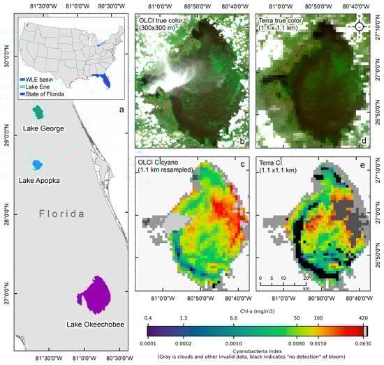
Figure 1.
An example of failure due to the saturation of MODIS CI bands over intense cyanobacteria blooms in Lake Okeechobee on 2 July 2018. (a) Location of the studied lakes, with the main map showing Lakes, Okeechobee, Apopka, and George in Florida (area enclosed by the red rectangle in the inset), and the inset showing the contiguous United States with study areas highlighted—western Lake Erie (WLE) basin in turquoise, Lake Erie in light blue, and the state of Florida in blue. (b) True-color OLCI image at native resolution (300 m) showing the presence of cyanobacteria biomass in high concentration, (c) Resampled CIcyano from OLCI, (d) True-color Terra image, and (e) Terra CI; darker gray in the east-central part of Lake Okeechobee in Terra CI image indicates failure due to saturated pixels, which corresponds to the intense bloom area in the OLCI image. Light and medium gray colors indicate clouds and land. Black color in panels (c) and (e) indicates “non-detect”; insufficient cyanobacteria for detection by the algorithms (see Section 2.1 for more information).
Establishing consistency among MODIS CI and MERIS/OLCI CIcyano is also a challenge as they are generated from three different sensors with different Full Width Half Maximum (FWHM) of needed bands and their band centers. Wynne et al. addressed this issue by intercalibrating MODIS CI with MERIS and OLCI CI using a simple linear regression approach [23]. To address a similar problem, [24] used a neural network approach to model a MODIS MCI product consistent with MERIS/OLCI MCI. They produced synthetic MERIS/OLCI-like bands centered at 681, 708, and 753 nm from MODIS bands as inputs to the neural net. They calculated a synthetic MODIS MCI in Lake Erie and two other Canadian lakes—Lake Winnipeg and Lake of the Woods. However, their neural network model needed to be regionally retrained for each lake [24].
In this study, our primary goal was to develop a generalizable method to fill the four-year gap of temporal data in the MERIS/OLCI CI time series using data from MODIS with machine learning (ML) approaches. Our specific objectives are:
- Develop a framework to generate a MODIS CIcyano time series that is consistent with MERIS/OLCI CIcyano and can be used to fill the four-year gap in the MERIS/OLCI CIcyano time series in Lake Okeechobee,
- Develop a method that can address the MODIS Red-NIR saturation issue over bright targets and minimizes the spatial data loss in the CIcyano products, and
- Independently validate the MODIS-generated CI in other lakes proving the replicability and geographic transferability of the model, without retraining, for broader application.
2. Materials and Methods
2.1. Satellite Data
2.1.1. MERIS/OLCI CIcyano Data
CIcyano products were derived from 300 m resolution data from the MERIS sensor onboard the Envisat satellite for 2002–2011 and from the OLCI sensor on the Copernicus Sentinel-3A for 2016–2020. We calculated spectral surface reflectance (ρs(λ); unitless) from MERIS and OLCI L1B data using NASA’s SeaDAS OCSSW data processing package (version msl12 9.5.1), the NASA standard software for processing ocean color data and projected it to an Albers projection and saved it as level 3 (L3) files. ρs(λ) data were determined by removing Rayleigh radiances and corrected for elevation from the instrument-observed top-of-atmosphere radiances, then converted to reflectance via normalizing with downwelling irradiance at the sea surface. Clouds and strong sun glints were masked using a cloud and glint detection algorithm [25]. Finally, we discarded adjacent pixels along each water body to avoid land adjacency issues, including mixed land/water pixels, and to ensure the signals originating from land vegetation were identified and excluded from further analysis [26]. The remaining pixels are termed “valid pixels”. The Cyanobacteria Index [8,11], a cyanobacterial biomass indicator, was calculated below (Equation (1)). The algorithm is explained in greater detail elsewhere [1,8,27,28] and briefly described here.
The Cyanobacteria Index in its original form was formulated as a spectral shape of the form of a second derivative centering 681 nm, SS (681) (Equation (1)), where it measured the 681 nm reflectance peak height from a baseline drawn between 665 nm and 709 nm bands [11]. A negative SS (681) represented the presence of cyanobacteria, which could be attributed to cyanobacteria having a much lower fluorescence signal at 681 nm than eukaryotic phytoplankton. In contrast, a positive SS (681) or a well-defined fluorescence peak around 681 nm described cyanobacterial absence or a CI of 0. [8] incorporated a second spectral shape, SS (665), to further confirm the cyanobacterial presence [8]. SS (665) was formulated to measure the reflectance peak height at 665 nm from a baseline drawn between 620 nm and 681 nm bands (Equation (1)). SS (665) uses the absorption feature of phycocyanin at 620 nm. Therefore, the elevated presence of phycocyanin-containing cyanobacteria enhances the 665 nm reflectance peak, causing SS (665) positive. Thus, SS (665) is used as a binary flag on top of the original CI product (|SS (681)|, when SS (681) < 0) to further confirm the presence of phycocyanin-bearing cyanobacteria in water bodies.
In Equation (1), ρs(x) indicates Rayleigh-corrected surface reflectance measured at a band with a bandcenter of x nm. Further, MERIS/OLCI 300 m data were resampled to 1100 m resolution to match MODIS Terra spatial resolution to compare the CIcyano time series from MERIS/OLCI and MODIS sensors.
2.1.2. MODIS Terra Data
We downloaded Level 0 MODIS Terra imagery from NASA. These images were then processed using NASA’s SeaDAS OCSSW data processing package (version msl12 9.5.1), the NASA standard software for processing to level 3 (L3) Rayleigh-corrected surface reflectance products. We used Terra instead of Aqua as Terra overpass time is within less than 90 min of MERIS and OLCI overpass times. Minimizing the difference in overpass time reduces the impact of vertical and horizontal movement of cyanobacteria blooms in a shallow lake like Lake Okeechobee. Moreover, reflectance data from Terra and Aqua agreed with each other within 2% for three bands (645 nm, 858 nm, and 1640 nm) for the years from 2002 to 2006 [29]. Therefore, surface reflectance measurements from Terra and Aqua are expected to match each other, although such a comparison is outside the scope of this current work.
2.2. Matchup Dataset
For robust model training and evaluation, we intended to develop a model that was trained with data from Lake Okeechobee and validated in other regions. After resampling native resolution MERIS images to match Terra, we extracted CIcyano pixel values for all 1100 × 1100 m pixels in Lake Okeechobee from May 2002 to December 2011 (MERIS) and April 2016 to June 2021 (OLCI). We excluded all pixels within 2 km from the lake shoreline to avoid land adjacency and mismatch due to differences in the data that can happen due to the resolution of the land mask (300 m for MERIS/OLCI vs. 1100 m for Terra). Thus, 832 interior pixels were extracted from each MERIS and OLCI CIcyano image. Similarly, we extracted Terra pixel values at those 832 pixels for each matching date. We then joined those datasets on a unique ID such that a unique MERIS/OLCI and Terra pixel would have a one-to-one match on a given image acquisition date. For quality assurance/quality control, no manual image selection was carried out. Instead, we used a semi-automatic Valid Pixel Fraction (VPF) approach. VPF is the fraction of valid pixels (those not contaminated by clouds, glint, etc., see Section 2.1.1) in the lake on a given day. With this information, we discarded an image date from the matchup dataset if the VPF was less than 50%. Although not perfect, this approach excludes images with heavy cloud cover or imagery contaminated by strong sun glint.
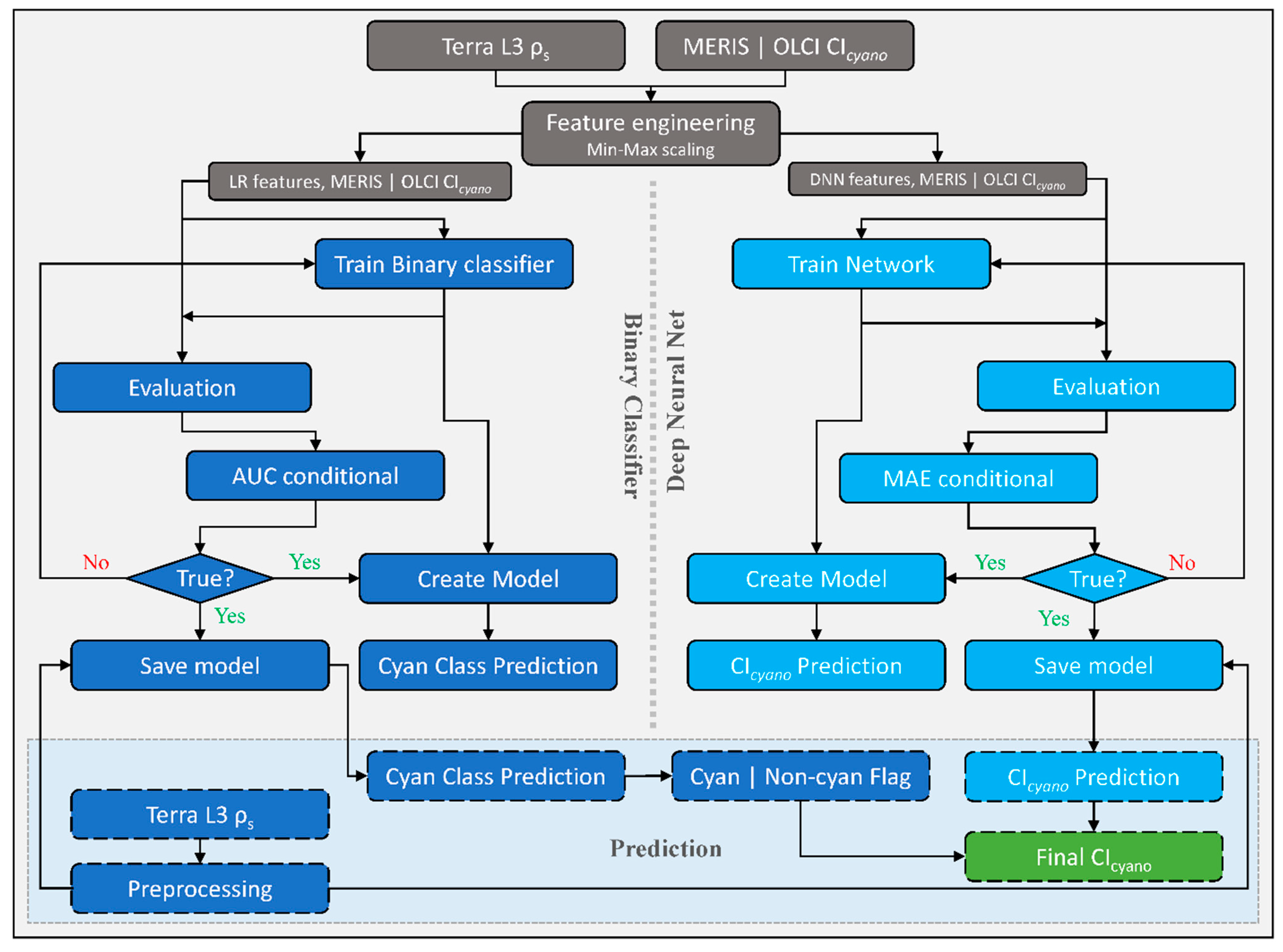
2.3. CyanNet Framework
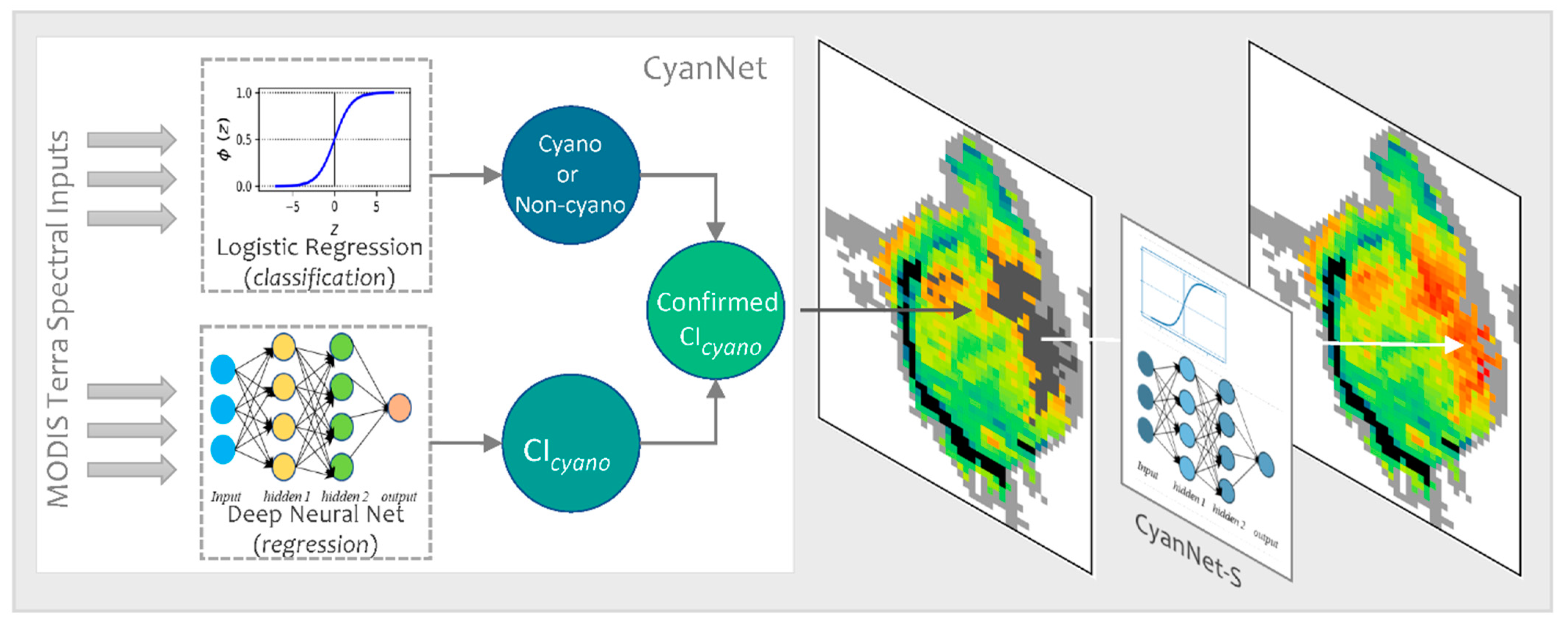
We designed the CyanNet framework by combining two models—A Logistic Regression (LR) classifier and a Deep Neural Network (DNN). LR model component uses 17 MODIS Terra spectral features (ρs and other derived features) to classify a pixel as a cyanobacteria pixel or a non-cyanobacteria. On the other hand, DNN uses 12 spectral features (ρs and other derived features) to predict the magnitude of CIcyano at the cyanobacteria classified pixel (Table 2). To address the MODIS band saturation issue over bright targets, we created a replicate of the CyanNet, CyanNet-S, that does not use the bands that saturate (Table 2). By design, CyanNet-S skips the red-NIR bands that tend to saturate over bright targets and returns a CIcyano retrieval over the saturated pixels when the standard CyanNet fails. While the CyanNet covers a full range of cyanobacteria concentrations, CyanNet-S typically only needs to address high-concentration biomass (where the bands saturate). Model components of the CyanNet framework are briefly discussed below.
Table 2.
Terra spectral features used in CyanNet. CyanNet-S, a replicate of CyanNet, uses fewer spectral features represented by LR-S and DNN-S.
- Logistic Regression classifier
Logistic Regression (LR) classifies a pixel in an image, given that they are linearly separable numeric samples, into a class or category, e.g., ‘Cyan’ and ‘Non-cyan’ class. Unlike other classifiers, LR outputs a probability (p)—a value between 0 and 1, exclusive, which can be used to define class membership. For example, if an LR model for cyanobacteria detection infers a p-value of 0.95 for a given pixel, it implies a 95% probability that it is a ‘Cyan’ pixel [30]. In this study, the LR classifier uses 17 Terra spectral features associated with Chl-a or blooms (Table 2) to classify a Terra L3 ρs file into a map of probability values of being cyanobacteria. Then, using a threshold, we converted the probability map into a binary ‘Cyan’ and ‘Non-cyan’ map (Figure 2, left of the dotted vertical line). We trained a replicate of LR—LR-S for saturated pixels using 13 spectral features that excluded the MODIS bands prone to saturation (Table 2).
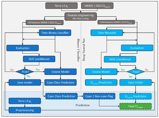
Figure 2.
Schematic diagram showing CyanNet train/test and prediction workflow as carried out in this study. The left side of the figure, highlighted in blue, shows the Logistic Regression (LR) classifier workflow, and the right side, highlighted in turquoise, shows the fully connected Deep Neural Network (DNN) workflow. Final retrievals of CIcyano from CyanNet are highlighted in green. CyanNet-S for saturated pixels replicates the same workflow with different LR and DNN features listed in Table 2.
- 2.
- Fully connected Deep Neural Network (DNN)
The DNN makes a continuous prediction and returns a map of CIcyano continuous values (Figure 2, flowchart part colored Cyan). Further, we use the binary flag from LR as a Cyan–Non-cyan binary flag to keep only Cyan-flagged pixels and convert the non-cyan pixels to 0. LR in CyanNet can be considered the cyanobacteria confirmation flag, equivalent to using the 665 nm band shape in the CIcyano algorithm (Equation (1)). We structured the DNN with three hidden layers containing 25 nodes, a fourth hidden layer with 12 nodes, and an output layer with one node. We scaled the MODIS spectral features listed in Table 2 with Min-Max scaling before feeding to the network. We trained the network using the model parameters provided in Table 3 in a Python environment. We used a rectified linear unit (ReLU) activation function for the hidden layers, a linear activation function for the output layer, and Mean Squared Error (MSE) as the loss function.
Table 3.
Model parameters used in neural network training. * ReLU = rectified linear unit.
In operation, a Terra ρs L3 file is passed through CyanNet, making a CIcyano prediction for each pixel. In the case of saturated pixels, the file is passed through CyanNet-S to make CIcyano predictions for the saturated pixels. The predictions from both frameworks are then merged into one final CIcyano file. CyanNet prediction workflow is summarized in Figure 3.
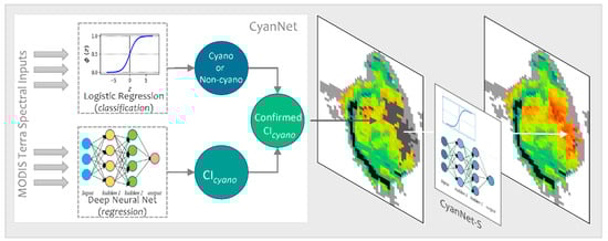
Figure 3.
CyanNet prediction workflow for unsaturated and saturated pixels in an example MODIS Tera image.
2.4. Model Evaluation
2.4.1. Model Training and Validation
Spatio-temporal processes such as cyanobacteria bloom events can have spatial and temporal autocorrelation, and therefore separating an independent dataset for model skill assessment is critical. Consequently, we omitted all data from 2009 and 2016 from the MERIS and OLCI time series from model training. Thus, the networks were trained with data from the other years and validated with data from 2009 and 2016.
2.4.2. Evaluation of Model with Composites
In large lakes with a long fetch, wind can play a critical role in circulation and cause noticeable differences in satellite observations during the two satellite’s overpass periods, even on the same-day matchup pairs. Thus, subtle differences in CI from MODIS and MERIS/OLCI are possible. To overcome this issue, we generated 10-day CI-max composites [31,32]. These types of composites are used to evaluate seasonal and annual variations in bloom intensity while reducing the influence of wind on the observed patterns [1,2,33]. As CIcyano values are in dimensionless “reflectance” units, without apparent physical meaning, we converted CIcyano to a nominal cyanobacterial Chl-a concentration using a CIcyano to Chl-a relationship developed for the lakes across the contiguous United States (CONUS) [34]
We did not include the intercept term from [34] as it was not meaningfully different from zero [34]. We also calculated the 10-day mean or annual bloom magnitude [7,27], representing the spatio-temporal mean Chl-a concentration in the lake. Finally, we compared the bloom magnitudes observed from MERIS/OLCI and MODIS-CyanNet for CyanNet skill assessment.
2.4.3. Model Evaluation for Geographic Transferability
The geographic transferability of the developed model is desirable as it shows the model’s generalization ability, or that the model is not specific to the lake for which it was trained. Model generalization power would also demonstrate the broader applicability without additional model tuning with a new dataset. We validated the model in two other lakes in Florida: Lake Apopka and Lake George (Figure 1a), by comparing mean Chl-a from the MERIS/OLCI and MODIS CyanNet 10-day max composites.
We also evaluated CyanNet in western Lake Erie (WLE) (Figure 1, inset), which has been frequently monitored and heavily studied for cyanoHABs. Evaluation in western Lake Erie confirms the models’ generalizability and ability to transfer the model to an independent geographic region. Here we compared the model performance on a selected set of 26 good-quality daily image pairs used in previous sensor intercalibration work [23].
2.4.4. Evaluation Metrics
We used median bias and median absolute difference (MedAD) to assess CyanNet performance, as provided below.
In Equations (3) and (4), M is the modeled CIcyano from CyanNet, and O is the CIcyano from MERIS/OLCI. The closer the multiplicative bias is to 1, the less bias the comparisons have and the better the model accuracy. For example, a bias of 1.1 indicates a model that overestimates by about 10%, and a mean bias of 0.9 suggests a model that underestimates by about 10%. Median bias quantifies the systematic difference between the modeled value (M) and the observed value (O). On the other hand, MedAD captures the difference in magnitude, highlighting the absolute difference between the observed and modeled CIcyano.
We used the area under the receiver operator characteristic (ROC) curve (AUC) metric [35,36] to evaluate LR classifier performance. AUC captures the ability of the model to separate a positive class (cyano pixel) from a negative class (non-cyano pixel). It is the most common metric used to evaluate binary classifiers in imbalanced datasets where one class is a majority class (non-cyanobacteria) with most of the data, and the other is a minority class (cyanobacteria) [37]. AUC represents the probability that a random bloom pixel is classified as a bloom pixel and ranges in value from 0 to 1. A classifier with an AUC of 1 is perfect with no errors. A classifier with an AUC of 0.5 is as good as a random classifier with a probability of detection accuracy of 50%. A model with an AUC of zero is always wrong.
3. Results
We evaluated the prediction accuracy of standard LR and DNN models in the CyanNet framework using the independent validation dataset from 2009 and 2016. The standard LR classifier produced an AUC of 0.91, accurately predicting cyanobacteria presence (Table 4). In comparison, LR-S had an AUC of 0.85 showing satisfactory performance. The standard DNN trained with the 12 Terra spectral features (Table 2) reliably predicted MERIS/OLCI equivalent CIcyano with a MedAD of 1.27. In other words, there is a 27% difference between the CyanNet-derived CIcyano and MERIS/OLCI CIcyano in the validation dataset from 2009 and 2016. The standard DNN model produced a median bias of 0.95 or a 5% negative bias. However, the mean bias in the linear scale is −0.0001 CIcyano which is the detection limit of the CIcyano algorithm. On the other hand, DNN-S, designed for the saturated pixels, predicted CIcyano with a MedAD of 1.41 and a negligible median bias of 1.003. The reduced performance of DNN-S (median absolute percent error of 33.6%) compared to standard DNN (median absolute percent error of 24.5%) is due to limited spectral information available to the DNN-S model. The exclusion of key red-NIR spectral channels due to saturation negatively affects the performance of DNN-S.
Table 4.
Logistic Regression (LR) binary classifier (Cyan–Non-cyan) and the Deep Neural Network (DNN) model accuracy as observed in the validation dataset from 2009 and 2016 through pixel-level matchup.
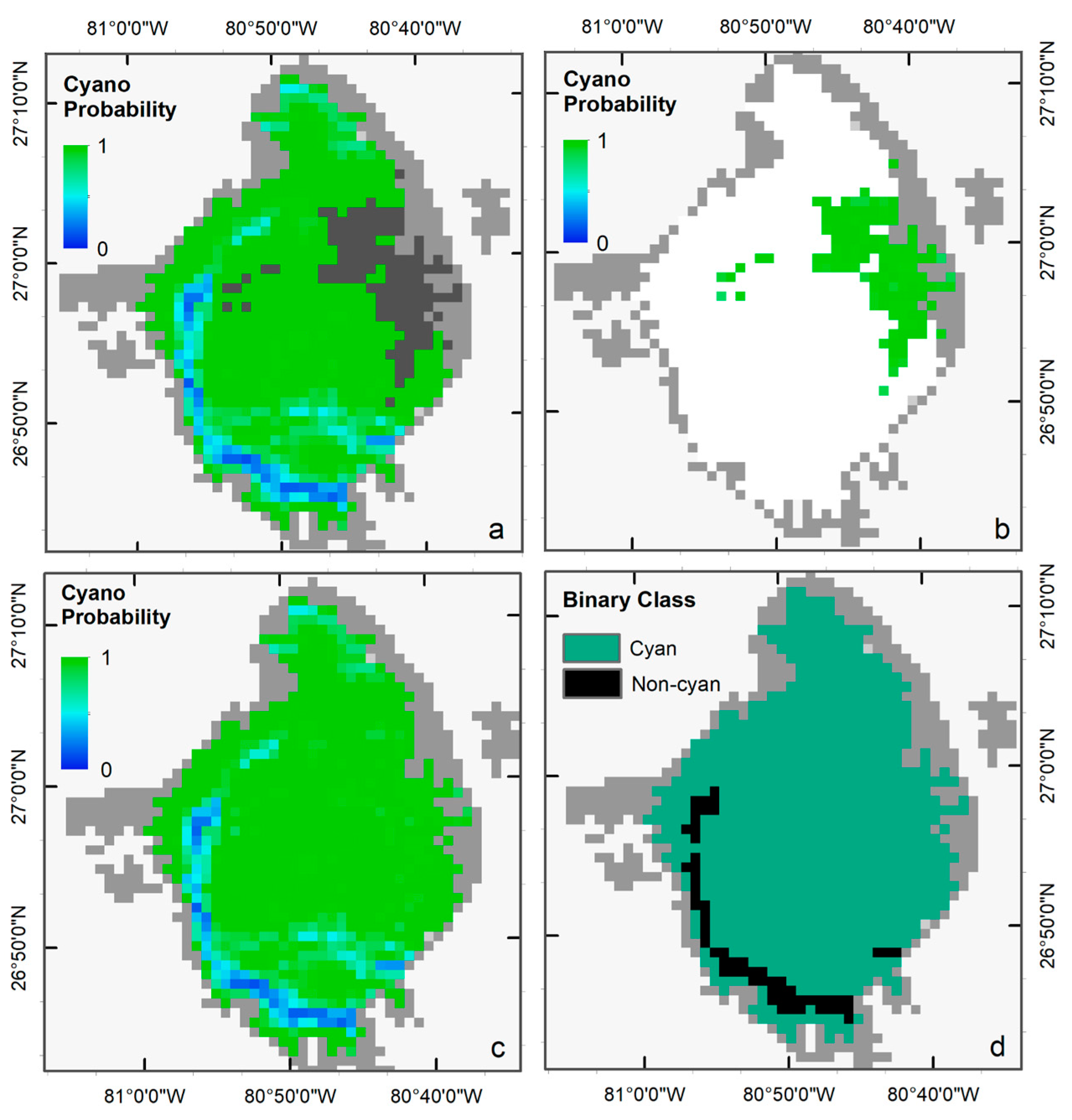
We selected the Terra image from 2 July 2018, to visually demonstrate the performance of the LR classifier in ‘Standard’ and ‘Saturated’ modes, as a significant portion of the image was affected by band saturation due to intense scattering from cyanoHAB surface scum (dark gray pixels in Figure 4a). Standard LR successfully generated a probability map of cyanobacteria presence for all pixels except over the saturated area. Similarly, LR-S was used to predict the probability of cyanobacteria presence over the saturated pixels (Figure 4b). The two probability maps were then merged to create a single map (Figure 4c). We used a threshold of 0.5 (cyanobacteria presence if p > 0.5, else absence) to classify the probability map into a binary cyanobacteria presence (cyan color) or absence (black color) map (Figure 4d).

Figure 4.
(a) Cyanobacteria probability map from the standard LR, and (b) and from LR-S classifier. (c) merged probability map from the two classifiers, and (d) the final binary map with Cyan AND Non-Cyan classes classified with a probability threshold of 0.5.
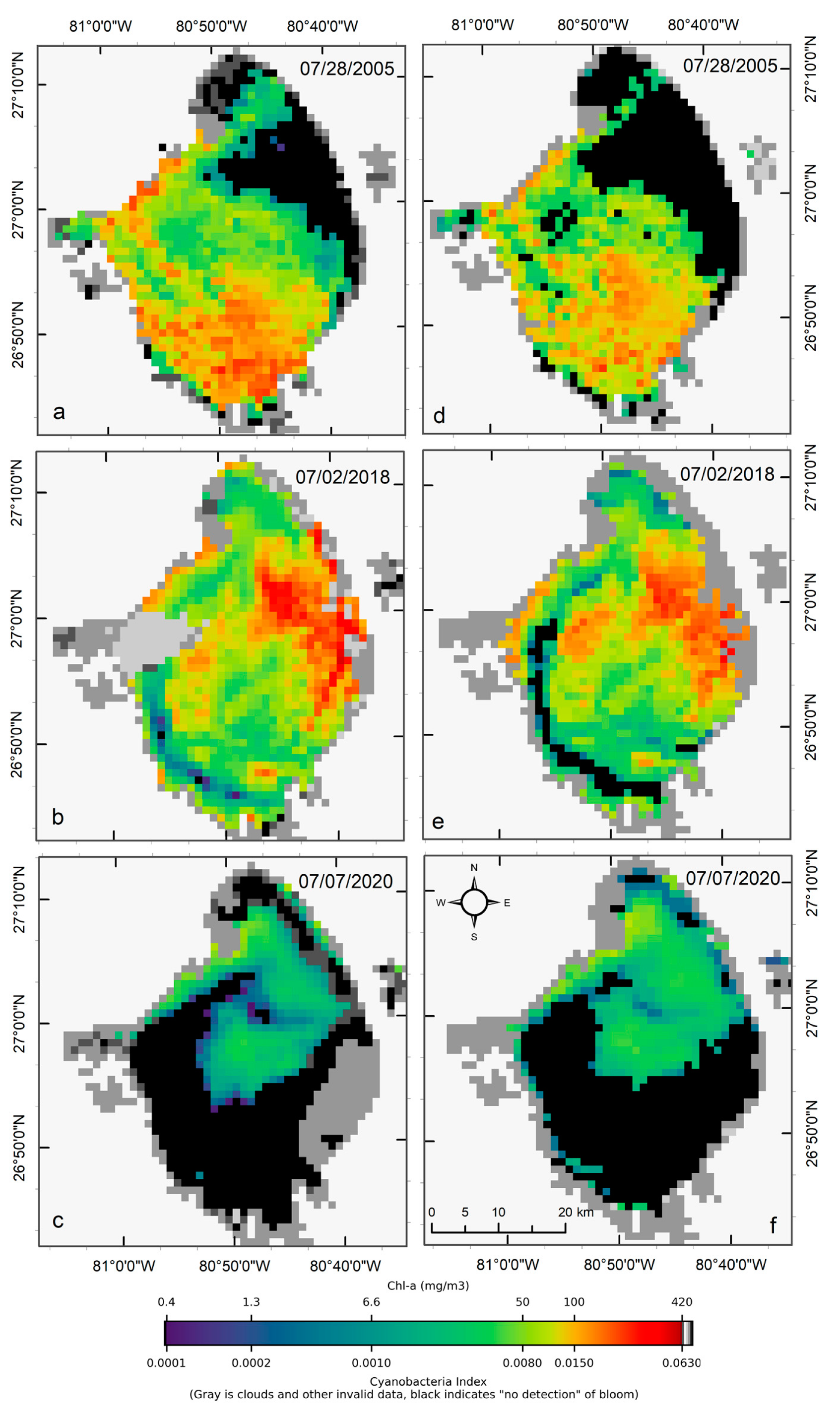
Visual comparisons of CIcyano products from MERIS/OLCI and Terra-CyanNet are provided in Figure 5. Spatial patterns and visual intensity of the bloom in MERIS CIcyano from 28 July 2005 matches very well with the CIcyano product from Terra (Figure 5a,d). The presence of surface scum in the southern part of the lake and western shoreline is consistent in both products. However, some mismatch is visible in the northern part of the lake. This could be due to the lower sensitivity of CyanNet in the low range of CIcyano. Also, shallow water systems like Lake Okeechobee are more affected by windy conditions than deeper lakes. Previously, a decrease in cyanobacteria bloom area and intensity has been linked with daily wind speed exceeding 7.7 m s−1 in western Lake Erie [33]. Similarly, in Lake Taihu, China, with a mean water depth of 1.9 m and surface area of 2339 km2, complete mixing throughout the water column was observed when wind speed exceeded 7 m s−1 [38]. In Lake Okeechobee, with a comparable surface area (1900 km2) and mean depth (2.7 m) to Lake Taihu, similar wind speeds between two satellite overpass times could cause vertical mixing and bloom movement contributing to the observed differences.

Figure 5.
Comparison of MERIS/OLCI derived CIcyano (a–c) with Terra CyanNet derived CIcyano (d–f) in Lake Okeechobee on the three selected dates. Light and medium gray colors indicate clouds and land. Black color indicates “non-detect”; insufficient cyanobacteria for detection by the algorithms.
OLCI and Terra CIcyano map from 2 July 2018, also match very well visually. High-biomass intensity surface scums are spatially consistent in both images (Figure 5b,e). As expected, very low CIcyano values along the southwest shoreline were classified as an absence of CIcyano in the Terra CyanNet image (Figure 5e). Similarly, the spatial pattern of the bloom in OLCI CIcyano (Figure 5c) and Terra CIcyano (Figure 5f) match very well. However, Terra CIcyano values appear to be slightly overestimated.
3.1. CyanNet Validation with 10-Day Composites
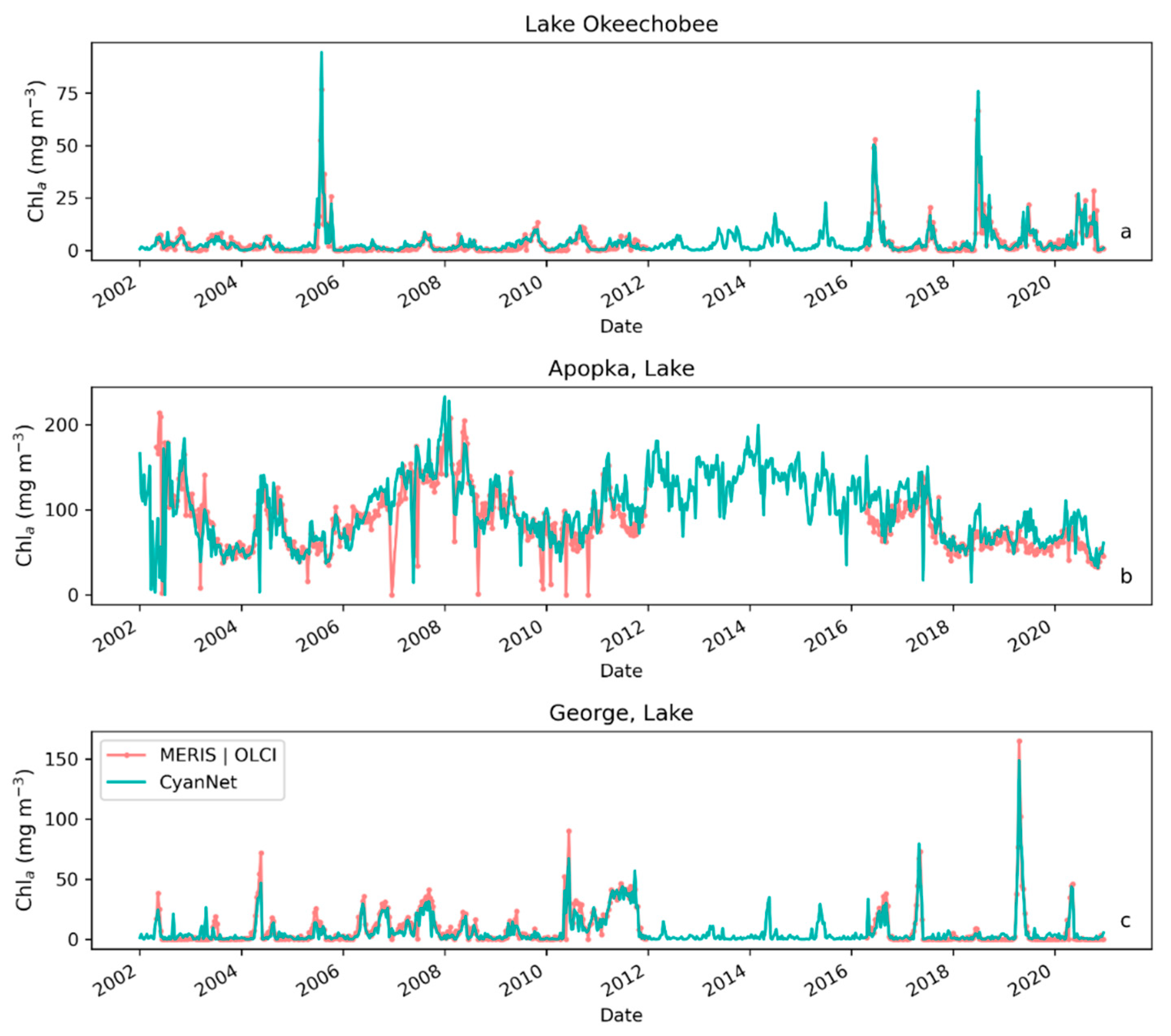
Examining seasonal and interannual variability of blooms is an important application of satellite data. As such, we examined the performance of CyanNet using 10-day composites generated from the time series. We compared the 10-day mean Chl-a concentration time series in Lake Okeechobee as predicted by CyanNet-CIcyano and from OLCI/MERIS CIcyano for February 2002–April 2012 and June 2016–June 2021 (Figure 6a). All available satellite data were included, so the products and analysis would include uncertainty in CIcyano data products from flagging failure (cloud, glint, land proximity, etc.) and mimics an operational lake monitoring framework. The 10-day mean Chl-a from Terra CyanNet tracked with the MERIS and OLCI mean Chl-a time series in the lake—detecting the peaks and troughs in the bloom time series. For example, high bloom years such as 2005, 2016, and 2018 are captured by the CyanNet product. The quantitative validation of the time series data produced a median bias of 0.87 and a MedAD of 36%. Put differently, CyanNet products overestimate the mean Chl-a by up to 36% (Figure 7a). Comparison of mean Chl-a time series resampled to annual means produced a better matchup with a MedAD of 17% and a 10% median positive bias (Figure 8a and Figure 9a).
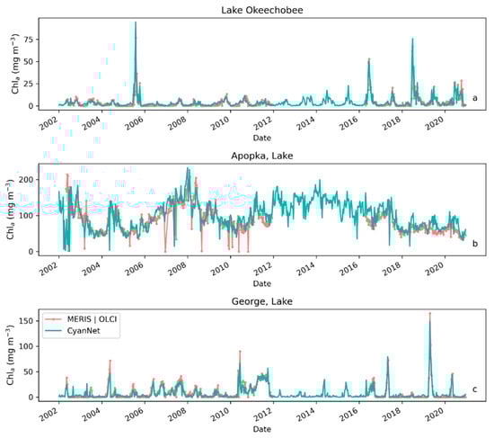
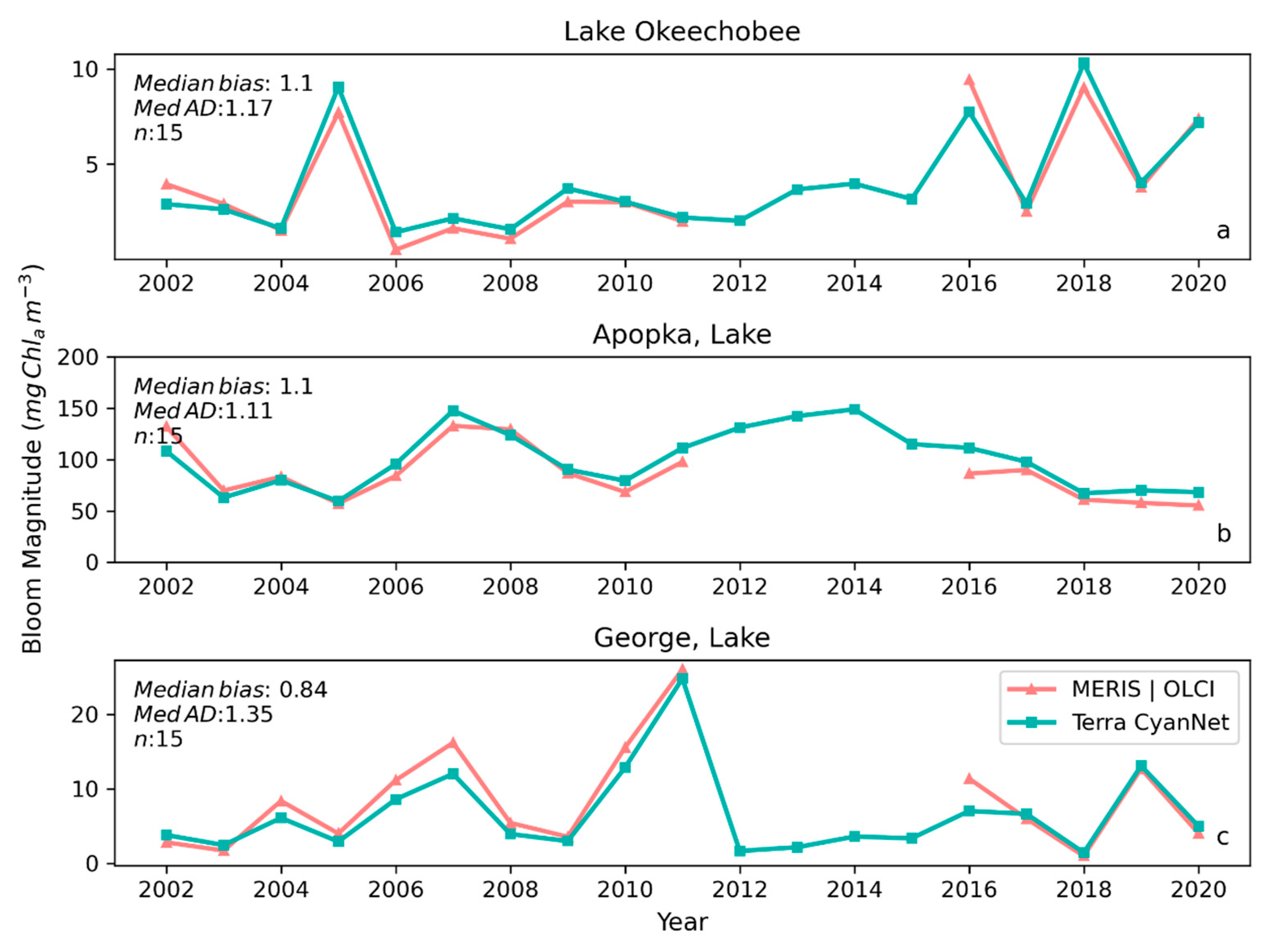
Figure 6.
Comparison between MERIS/OLCI derived 10-day composite Chl-a time series and that from Terra with CyanNet in (a) Lake Okeechobee, (b) Lake Apopka, and (c) Lake George in Florida.

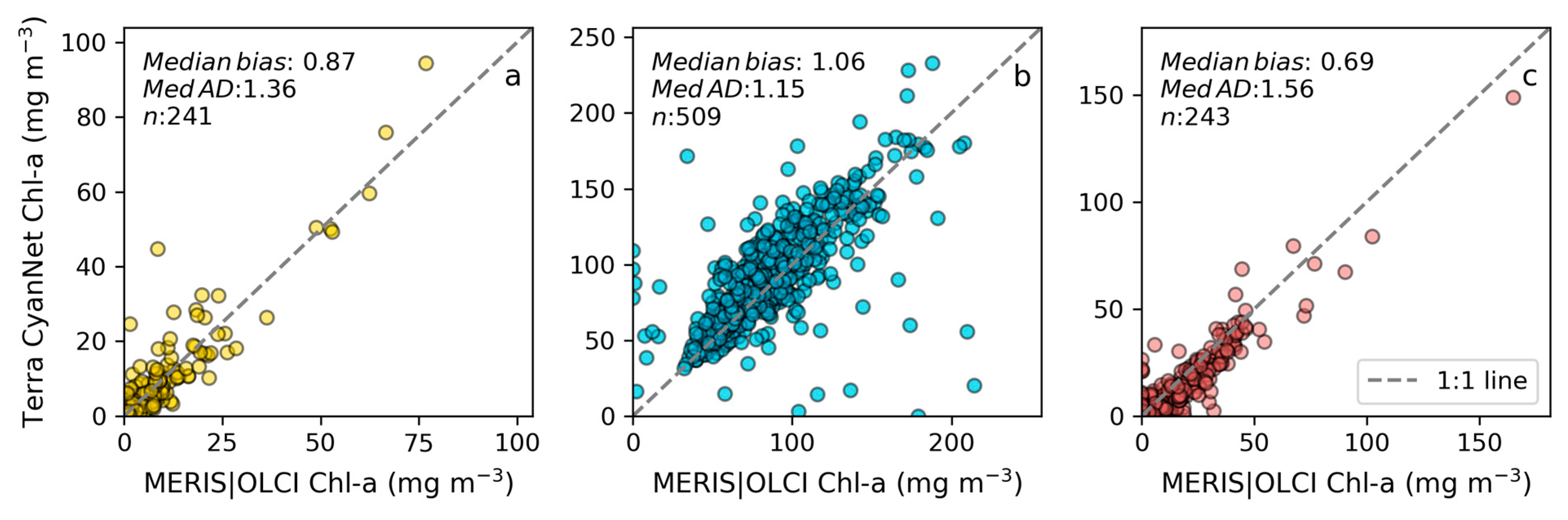
Figure 7.
Comparison between MERIS/OLCI derived mean Chl-a and that from Terra with CyanNet from 10-day composites in (a) Lake Okeechobee, (b) Lake Apopka, and (c) Lake George in Florida.
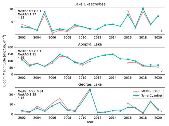
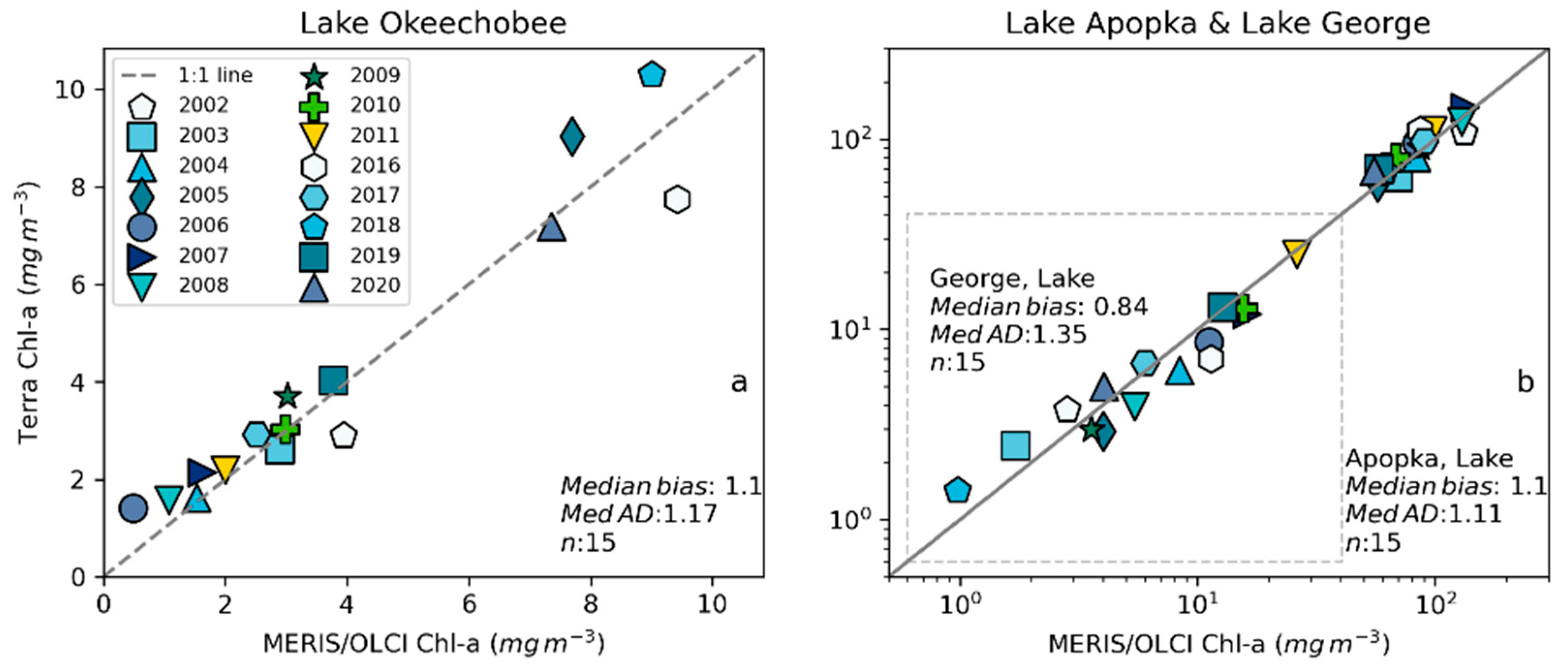
Figure 8.
Comparison between annual bloom magnitudes observed from MERIS and OLCI 10-day time series and Terra-CyanNet 10-day composite time series in (a) Lake Okeechobee, (b) Lake Apopka, and (c) Lake George. Significant underestimation in Terra CyanNet bloom magnitude in Lake George in 2007, and 2016 is due to heavy cloud cover in Terra data during the peak of the bloom season. Significant overestimation in Terra CyanNet bloom magnitude in Lake Okeechobee in 2005 and 2018 is due to more data coverage compared to MERIS and OLCI; overestimation in Lake Apopka in 2007 and 2016 is primarily due to cloud and sun glint flagging issues in MODIS data.

Figure 9.
Validation with annual bloom magnitudes observed from MERIS and OLCI 10-day time series and Terra-CyanNet 10-day composite time series in (a) Lake Okeechobee and (b) Lake Apopka and Lake George (surrounded by dashed gray rectangle).
We validated CyanNet in Lake Apopka and Lake George without regional tuning. Like Lake Okeechobee, the 10-day mean Chl-a time series in Lake Apopka from Terra CyanNet tracked very well with the 10-day mean Chl-a time series from MERIS and OLCI. The CyanNet time series captured the annual peak bloom events detected by MERIS/OLCI CIcyano, especially in the high magnitude bloom years in 2005, 2007, and 2017. Overall, CyanNet still produced a small overestimate of the mean Chl-a concentration (about 15%) (Figure 7b). For Lake Apopka, discrepancies occur when MERIS/OLCI mean Chl-a concentration approaches zero in the 10-day composite time. Those data points with the highest mismatch are due to spatial data gaps in MERIS/OLCI and Terra time series (Figure S1). Outliers in Chl-a time series in both MERIS/OLCI and TERRA CyanNet Chl-a time series overlap with invalid data fraction in Lake Apopka in the 10-day composites confirming the mismatch is due to the limited data availability (Figure S1). The fraction of invalid data in both sensors should be considered in data analysis. Excluding composites with a large fraction of invalid data, the annual mean magnitude from CyanNet in Lake Apopka matched well with mean magnitudes from MERIS and OLCI with a MedAD of 11% and a median positive bias of 10% (Figure 8b and Figure 9b).
Finally, CyanNet mean Chl-a in Lake George from the 10-day composites matched reasonably well with the mean Chl-a from MERIS and OLCI 10-day composites. CyanNet captured the peak bloom events well, especially in 2004, 2007, 2011, 2017, and 2019. CyanNet underestimated MERIS/OLCI mean Chl-a with about 30% negative bias. The MedAD between the two-time series is 56%. However, most of the Chl-a predictions are less than 5 mg m−3, where percent error tends to make it appear very high, although the absolute difference in half of the samples is less than 2 mg m−3 (median difference = 1.97 mg m−3). Comparison of annual bloom magnitude matched better than the mean Chl-a concentrations from the 10-day composites. The median difference between the two-time series was 35%, with a 16% negative median bias (Figure 8c and Figure 9b). A noticeable difference between the annual bloom magnitudes derived from CyanNet and MERIS/OLCI is observed in 2007 and 2016 (Figure 8c and Figure 9b). Heavy cloud cover obscured the MODIS-Terra data during the peak bloom days, causing an underestimation of bloom magnitude for those years.
3.2. Validation in Lake Erie
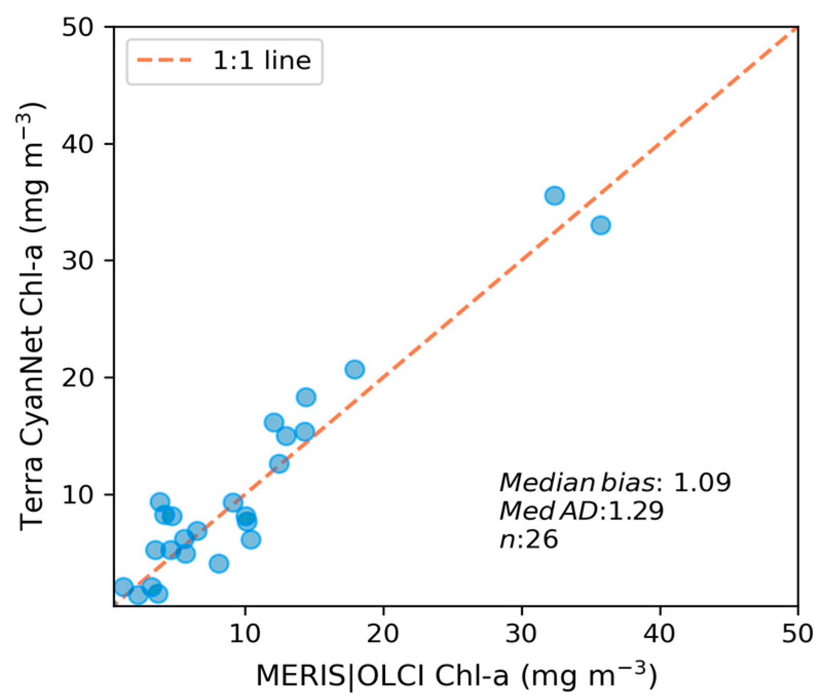
We transferred CyanNet to western Lake Erie without further regional training and validation. We evaluated the model with 26 daily CIcyano image pairs from MERIS/OLCI and Terra-CyanNet. CIcyano spatial patterns from CyanNet matched very well with MERIS/OLCI (Figure 10). However, some discrepancy in the lower end of CIcyano is visible, potentially due to a cyano-flagging issue. For example, the MERIS CIcyano product misses low-biomass pixels due to more conservative cyan/non-cyan flagging by the 665 nm shape in the CIcyano algorithm (Figure 10a, red annotated area). In contrast, the CyanNet LR classifier classifies those pixels as valid cyan pixels. Similarly, low-biomass OLCI CIcyano pixels from 23 September 2017, in the same area are flagged by potential land adjacency. CyanNet keeps those pixels as valid data, as CyanNet does not use the land adjacency flag. On 18 August 2022, the data show how CyanNet could lose low-biomass CIcyano pixels, classified as non-cyan pixels. On the same day, OLCI CIcyano identified the low-biomass bloom area (Figure 10c,f, red annotated area). With all these discrepancies in the low end, quantitatively, daily mean Chl-a concentrations from MERIS/OLCI and Terra differed by 29% with a 9% positive bias (Figure 11).
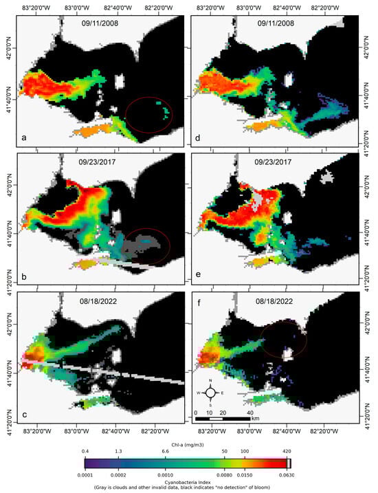
Figure 10.
Comparison of MERIS/OLCI derived CIcyano (a–c) with CyanNet derived CIcyano (d–f) in the western Lake Erie basin on the three selected dates. Red circles in panels a-b highlight the pixels missed by CIcyano but are detected as cyanobacteria presence in low concentration in the Terra CyanNet CIcyano image. In contrast, the red circle in panel f shows the opposite. Light and medium gray colors indicate clouds, invalid data, and land. Black color indicates “non-detect”; insufficient cyanobacteria for detection by the algorithms.
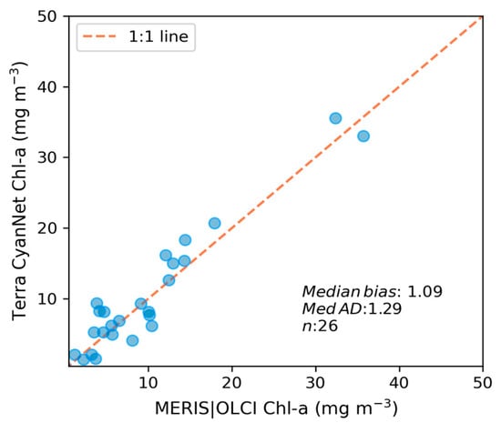
Figure 11.
Assessment of CyanNet derived CIcyano in the western Lake Erie basin.
3.3. Continuous and Consistent Bloom Time Series in Lake Okeechobee
We processed all available MODIS Terra daily data to predict MODIS CIcyano. No image screening was conducted to exclude images contaminated with either cloud cover or sun glint. We then validated the model performance in three different ways:
- A qualitative match-up between the observed and modeled time series, which is often used to show if the predictions are temporally consistent and represent the critical bloom phenological events.
- Quantitative validation of the retrievals from 10-day composites through scatter plots with error metrics.
- Quantitative validation of annual bloom magnitudes or annual mean Chl-a concentrations.
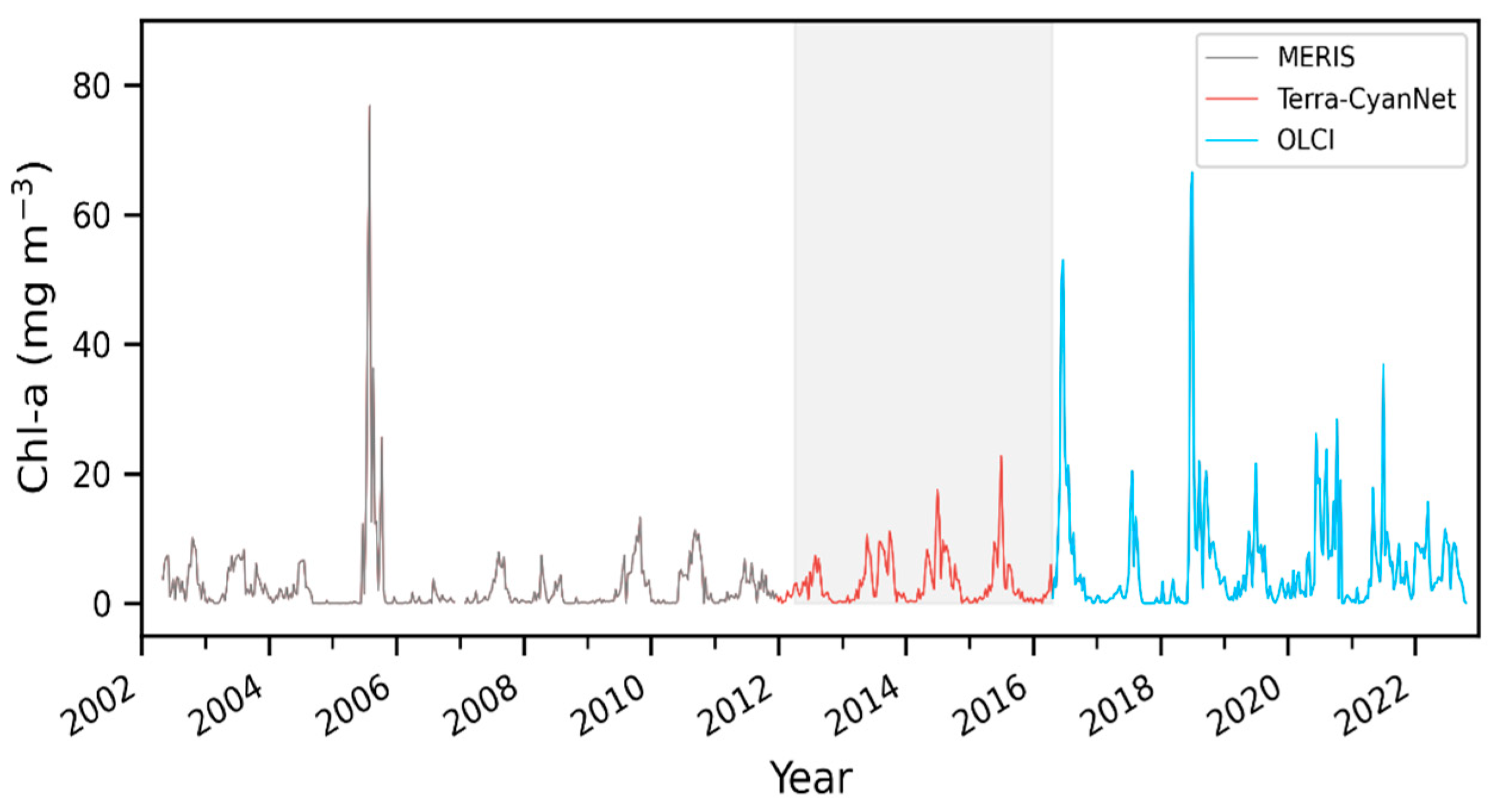
MODIS produced similar temporal and spatial patterns in the CIcyano as observed by MERIS and OLCI. Furthermore, all validation exercises demonstrated that MODIS CIcyano from CyanNet had acceptable differences compared to MERIS and OLCI, and, therefore, it would reliably fill the time series gap between those two sensors. Consequently, we merged the 10-day CIcyano time series from MERIS (2002–2011), MODIS-CyanNet (January 2012–April 2016), and OLCI (April 2016–October 2022) to create 21 years of consistent and continuous CIcyano time series in Lake Okeechobee (Figure 12). The continuous CIcyano time series data can be further used for retrieving cyanobacteria bloom phenological metrics in the lake, which can be beneficial in characterizing the timing of the annual key bloom events.

Figure 12.
21 years of continuous and consistent 10-day Chl-a timeseries from MERIS, MODIS, and OLCI in Lake Okeechobee. Shaded region shows the satellite observation discontinuity between MERIS and OLCI.
4. Discussion
4.1. Sources of Differences and Uncertainties
We processed the entire time series of MERIS (2002–2011) and OLCI (2016–2020) data, mimicking an operational lake monitoring setup for CyanNet’s skill assessment. Intentionally, we did not screen nor omit daily MODIS-Terra data due to cloud cover or sun glint contamination. Therefore, the performance of CyanNet presented here shows the worst-case scenario. Most of the differences were observed in the low range, where the differences are due to:
- The lower sensitivity of CyanNet in the lower end (<2 × 10⁻⁴ CIcyano).
- The difference in availability of valid data in the 10-day composites.
- Mismatch due to pixel flagging as valid/invalid data (clouds, sun glint, land adjacency) as well as the cyan flag, which is part of the CIcyano algorithm.
CIcyano algorithm cyan flag tends to follow a conservative approach while confirming a cyan pixel. On the other hand, CyanNet uses its flag generated by the LR classifier embedded in the framework. The classifier is designed to flag any pixel with a CIcyano value ≤ 1 × 10⁻⁴ as a non-cyan pixel. Therefore, it is possible that MERIS/OLCI CIcyano can have pixels with a value ≤ 1 × 10⁻⁴, and CyanNet flags them as non-cyan.
The invalid data fraction (%) difference between Terra and MERIS/OLCI significantly contributed to the MedAD between the two products (Figure S2). As expected, the sensor time series with more valid data tends to have a higher accumulated Chl-a. Therefore, in an ideal situation with the same spatial coverage from MERIS/MODIS and OCLI/MODIS, the degree of match-up would be better than in the current scenario. For example, in Lake George, out of 243 composites, only 72 composites had near-complete valid data (<1% difference in invalid data fraction between the two different time series). Nevertheless, a match-up with the selected data (<1% difference) improved the MedAD from 56% with 30% negative bias in all data to 17% with 10% negative bias (Figure S3c). Improvement in the match-up corroborates that valid data availability is critical in validating or comparing cyanobacteria Chl-a biomass from two sensors with different spatial resolutions and revisit times. It should be noted in the same analysis that match-up performance did not change in Lake Apopka, as the difference in valid data availability is not an issue in that lake. Less than 10% of composites had a difference of ≥ 1% in invalid data coverage (Figure 6b, Figures S2 and S3). However, the MedAD in Lake Okeechobee increased in the selected match-up dataset (with <1% difference in invalid data coverage) from 36% in all composites to 58%. That is primarily because out of 23 composites, 20 had less than 2 mg m−3 Chl-a, and the other two had a mean Chl-a concentration of 2–5 mg m−3. As discussed earlier, percent difference is not a good metric for evaluating the difference in the low end, as a meaningless difference could cause a very high percent error. Moreover, Chl-a retrievals below 2 mg m−3 would remain in the algorithm uncertainty range [7].
Significant differences occurred when one image had invalid data due to cloud, image cut lines (generated from image granule mosaicking), and windy conditions within the overpass difference time. Terra’s cloud and sun glint flags greatly affected the performance of CyanNet prediction. A pixel with a thin cloud missed by the cloud flag and unflagged sun glint-contaminated pixels caused erroneous CIcyano retrievals with significant overestimation. Thus, most overestimations in the CyanNet retrievals are most likely due to missed sun glint and cloud flags. Sun glint causes problems for many remote sensing algorithms, including CI, because it leads to overestimating ρs (λ) and modifies its spectral shape [21]. Currently, invalid data flags for OLCI are more robust than MODIS due to better spatial and spectral resolution [25]. In the future, more accurate flagging of invalid data in MODIS-Terra images could significantly improve the match-up.
4.2. CyanNet’s Novel Contribution and Its Broader Application
CIcyano modeled from MODIS Terra data using CyanNet matched well with CIcyano computed from MERIS and OLCI sensors with a dedicated 620 nm phycocyanin detection band. Temporal patterns of cyanobacteria bloom time series, such as bloom peaks and overall progression of bloom seasons, were well-captured by MODIS CIcyano. Moreover, the absolute difference between the MERIS/OLCI and modeled Terra Chl-a time series was within 36%, which included the inherent differences due to spatial and temporal coverage of valid data over the observed lakes. With CIcyano retrievals consistent with MERIS and OLCI CIcyano, CyanNet helped us create a continuous and consistent CIcyano time series from 2002 to 2022 in Lake Okeechobee (Figure 12), which could be used for retrieving bloom phenology, studying the climatology of cyanobacteria blooms, and its seasonal forecasting.
CyanNet addresses several limitations of MODIS CI, which is generated by simply replacing the MERIS/OLCI bands with the closest MODIS bands in Equation (1).
- Cyanobacteria confirmation: MERIS/OLCI CIcyano uses a cyanobacteria confirmation flag derived from spectral absorption features of phycocyanin, a characteristic photosynthetic pigment in cyanobacteria. MODIS CI does not use the flag as the 620 nm band is missing in MODIS [19]. However, CyanNet CIcyano fills that gap by applying a cyan/non-cyan flag to the predicted CI values from the DNN.
- CIcyano retrieval over Red/NIR band saturated areas: One of the limitations of MODIS CI is that the MODIS Red/NIR bands, especially the 678 nm band used in MODIS CI, saturate over bright targets such as intense algal blooms with a surface accumulation of cyanobacteria biomass due to high sensitivity and low saturation threshold [15,16,21]. Moradi (2014) stated that the MODIS CI could serve as an equivalent product of MERIS CI over cyanobacterial patches with ≤ 106 cell L−1 in the southern Caspian Sea [16]. CyanNet reduces that data loss by using the CyanNet-S to retrieve MODIS CIcyano, with the MODIS bands that tend not to saturate over bright targets.
- Consistency among CIcyano from different sensors: MODIS CI, calculated from the spectral shape (Equation (1) with closest MODIS bands) [16,39], shows similar spatial bloom patterns as in MERIS CI. However, because this requires substituting the MODIS 748 nm band for the MERIS/OLCI 709 nm, the magnitude of CI differs significantly between the two sensors. Therefore, MODIS CI requires further calibration to make it consistent with MERIS/OLCI CIcyano [16,23]. However, intercalibration of MODIS CI and MERIS/OLCI CI can sometimes be challenging with a linear-regression approach as non-linear trends are possible in the low end. CyanNet addresses that challenge and models MODIS CIcyano in the entire range consistent with MERIS/OLCI CIcyano.
The CyanNet framework may be suitable for modeling other MERIS/OLCI bloom indices from MODIS, such as MCI, MPH, and NDCI to fill the temporal gap from 2012 to early 2016. Unlike Zeng and Binding’s method [24] for filling the gap for an MCI, CyanNet does not need recalibration for different lakes or geographic regions. The effectiveness of CyanNet may be partially due to the inputs of spectral shapes that are consistent with both the CI algorithm and intense blooms. That may be one reason the CyanNet is generalizable to multiple lakes without retraining. Moreover, Binding et al. [40] applied Zheng and Binding’s method in Lake of the Woods but did not fully validate the modeled MCI to confirm the consistency of bloom severity in Lake of the Woods. Instead, they compared the bloom areas for the lake retrieved from MODIS and OLCI. In contrast, CyanNet retrieves the spatial extent (through cyan/non-cyan flag) and the intensity of the bloom, letting us estimate and validate both the bloom spatial extent (area) and magnitude of the bloom.
5. Conclusions
Combining multiple satellite missions to produce a continuous, decades-long-time series is critical in the long-term monitoring of biogeochemical parameters such as Chl-a in coastal and inland water bodies. To address this issue, we developed a machine learning solution—CyanNet, a fully connected deep neural net, to predict MERIS-OLCI-equivalent CIcyano in Lake Okeechobee from MODIS Terra data. The model performance was satisfactory, with a 17% median absolute difference in Lake Okeechobee annual bloom magnitude. The median difference was ~36%, with mean Chl-a observed from 10-day composite time series data, with differences often due to variations in valid data availability, clouds or glint. In addition, MODIS produced temporal and spatial patterns in the CIcyano observed in MERIS and OLCI, indicating that it would reliably fill the gap between these two sensors. Without further regional training, the same network performed well in Lake Apopka, Lake George, and western Lake Erie. Validation success, especially in Lake Erie, shows the model’s generalizability and transferability to other geographic regions. This extension to different areas also validates the potential robustness of the resulting model under various conditions.
Supplementary Materials
The following supporting information can be downloaded at: https://www.mdpi.com/article/10.3390/rs15225291/s1, Figure S1. Correspondence between Chl-a concentration from 10-day composites (solid lines) and the percentage of invalid data in the lake in the corresponding 10-day composite (dotted lines) in Lake Apopka. Note the extreme underestimations in MERIS/OLCI and Terra CyanNet Chl-a, where the time series overlaps with a high fraction of invalid data in the 10-day composites. Figure S2. Correspondence between the difference in Chl-a from Terra-CyanNet and MERIS/OLCI and the difference between the invalid data fraction (%) between those two time series in (a) Lake Okeechobee, (b) Lake Apopka, and (c) Lake George. A positive Chl-a difference indicates Terra retrieved higher Chl-a than MERIS/OLCI, and a positive invalid data fraction difference indicates Terra had more invalid data than MERIS/OLCI. The sensor with more invalid data tends to have a lower accumulated Chl-a, such that positive blue (more invalid data in Terra) has negative red (lower accumulated Chl-a from Terra), and negative blue (MERIS or OLCI more invalid data) has positive red (Terra higher accumulated Chl-a). Figure S3. Comparison between MERIS/OLCI derived 10-day Chl-a and that from Terra with CyanNet only when the difference in invalid data fraction (%) in the lakes was <1% in (a) Lake Okeechobee, (b) Lake Apopka, and (c) Lake George in Florida.
Author Contributions
Conceptualization, S.M. and R.P.S.; methodology, S.M.; software, S.M.; validation, S.M. and R.P.S.; formal analysis, S.M.; investigation, S.M.; resources, R.P.S.; data curation, A.M.; writing—original draft preparation, S.M.; writing—review and editing, S.M., R.P.S. and A.M.; visualization, S.M.; funding acquisition, R.P.S. All authors have read and agreed to the published version of the manuscript.
Funding
This work was sponsored by the U.S. Army Corps of Engineers’ Aquatic Nuisance Species Research Program (agreement number: W81EWF21876042), and partially supported by Great Lakes Restoration Initiative (GLRI), https://glri.us/projects (accessed on 9 September 2023), through the NOAA Decision Support Tools project, “Decision support tools to link nutrient reductions to harmful algal blooms”.
Data Availability Statement
All ocean color datasets from MODIS, MERIS, and OLCI are publicly available from the National Aeronautics and Space Administration (NASA) and the European Space Agency (ESA), and Copernicus Sentinel program.
Acknowledgments
Mention of trade names or commercial products does not constitute endorsement or recommendation for use by the US Government. The views expressed in this article are those of the authors and do not necessarily reflect the views or policies of the NOAA. The authors declare no competing interests.
Conflicts of Interest
The authors declare no conflict of interest.
References
- Stumpf, R.P.; Wynne, T.T.; Baker, D.B.; Fahnenstiel, G.L. Interannual variability of cyanobacterial blooms in Lake Erie. PLoS ONE 2012, 7, e42444. [Google Scholar] [CrossRef] [PubMed]
- Schaeffer, B.A.; Urquhart, E.; Coffer, M.; Salls, W.; Stumpf, R.P.; Loftin, K.A.; Werdell, P.J. Satellites quantify the spatial extent of cyanobacterial blooms across the United States at multiple scales. Ecol. Indic. 2022, 140, 108990. [Google Scholar] [CrossRef] [PubMed]
- Kutser, T.; Soomets, T.; Toming, K.; Uiboupin, R.; Arikas, A.; Vahter, K.; Paavel, B. Assessing the Baltic Sea Water Quality with Sentinel-3 OLCI Imagery. In Proceedings of the 2018 IEEE/OES Baltic International Symposium (BALTIC), Klaipeda, Lithuania, 12–15 June 2018; pp. 1–6. [Google Scholar]
- William Matthews, M. Near-term forecasting of cyanobacteria and harmful algal blooms in lakes using simple univariate methods with satellite remote sensing data. Inland Waters 2022, 13, 62–73. [Google Scholar] [CrossRef]
- Binding, C.; Pizzolato, L.; Zeng, C. EOLakeWatch; delivering a comprehensive suite of remote sensing algal bloom indices for enhanced monitoring of Canadian eutrophic lakes. Ecol. Indic. 2021, 121, 106999. [Google Scholar] [CrossRef]
- Coffer, M.M.; Schaeffer, B.A.; Darling, J.A.; Urquhart, E.A.; Salls, W.B. Quantifying national and regional cyanobacterial occurrence in US lakes using satellite remote sensing. Ecol. Indic. 2020, 111, 105976. [Google Scholar] [CrossRef] [PubMed]
- Mishra, S.; Stumpf, R.P.; Schaeffer, B.A.; Werdell, P.J. Recent changes in cyanobacteria algal bloom magnitude in large lakes across the contiguous United States. Sci. Total Environ. 2023, 897, 165253. [Google Scholar] [CrossRef] [PubMed]
- Lunetta, R.S.; Schaeffer, B.A.; Stumpf, R.P.; Keith, D.; Jacobs, S.A.; Murphy, M.S. Evaluation of cyanobacteria cell count detection derived from MERIS imagery across the eastern USA. Remote Sens. Environ. 2015, 157, 24–34. [Google Scholar] [CrossRef]
- Mishra, S.; Mishra, D.R.; Lee, Z.; Tucker, C.S. Quantifying cyanobacterial phycocyanin concentration in turbid productive waters: A quasi-analytical approach. Remote Sens. Environ. 2013, 133, 141–151. [Google Scholar] [CrossRef]
- Stumpf, R.P.; Davis, T.W.; Wynne, T.T.; Graham, J.L.; Loftin, K.A.; Johengen, T.H.; Gossiaux, D.; Palladino, D.; Burtner, A. Challenges for mapping cyanotoxin patterns from remote sensing of cyanobacteria. Harmful Algae 2016, 54, 160–173. [Google Scholar] [CrossRef]
- Wynne, T.T.; Stumpf, R.P.; Tomlinson, M.C.; Warner, R.A.; Tester, P.A.; Dyble, J.; Fahnenstiel, G.L. Relating spectral shape to cyanobacterial blooms in the Laurentian Great Lakes. Int. J. Remote Sens. 2008, 29, 3665–3672. [Google Scholar] [CrossRef]
- Gower, J.; King, S.; Borstad, G.; Brown, L. Detection of intense plankton blooms using the 709 nm band of the MERIS imaging spectrometer. Int. J. Remote Sens. 2005, 26, 2005–2012. [Google Scholar] [CrossRef]
- Matthews, M.W.; Bernard, S.; Robertson, L. An algorithm for detecting trophic status (chlorophyll-a), cyanobacterial-dominance, surface scums and floating vegetation in inland and coastal waters. Remote Sens. Environ. 2012, 124, 637–652. [Google Scholar] [CrossRef]
- Mishra, S.; Mishra, D.R. Normalized difference chlorophyll index: A novel model for remote estimation of chlorophyll-a concentration in turbid productive waters. Remote Sens. Environ. 2012, 117, 394–406. [Google Scholar] [CrossRef]
- Wynne, T.T.; Stumpf, R.P.; Briggs, T.O. Comparing MODIS and MERIS spectral shapes for cyanobacterial bloom detection. Int. J. Remote Sens. 2013, 34, 6668–6678. [Google Scholar] [CrossRef]
- Moradi, M. Comparison of the efficacy of MODIS and MERIS data for detecting cyanobacterial blooms in the southern Caspian Sea. Mar. Pollut. Bull. 2014, 87, 311–322. [Google Scholar] [CrossRef] [PubMed]
- Cannizzaro, J.P.; Barnes, B.B.; Hu, C.; Corcoran, A.A.; Hubbard, K.A.; Muhlbach, E.; Sharp, W.C.; Brand, L.E.; Kelble, C.R. Remote detection of cyanobacteria blooms in an optically shallow subtropical lagoonal estuary using MODIS data. Remote Sens. Environ. 2019, 231, 111227. [Google Scholar] [CrossRef]
- Zhang, F.; Hu, C.; Shum, C.; Liang, S.; Lee, J. Satellite remote sensing of drinking water intakes in Lake Erie for cyanobacteria population using two MODIS-based indicators as a potential tool for toxin tracking. Front. Mar. Sci. 2017, 4, 124. [Google Scholar] [CrossRef]
- Konik, M.; Bradtke, K.; Stoń-Egiert, J.; Soja-Woźniak, M.; Śliwińska-Wilczewska, S.; Darecki, M. Cyanobacteria Index as a Tool for the Satellite Detection of Cyanobacteria Blooms in the Baltic Sea. Remote Sens. 2023, 15, 1601. [Google Scholar] [CrossRef]
- Simis, S.G.; Peters, S.W.; Gons, H.J. Remote sensing of the cyanobacterial pigment phycocyanin in turbid inland water. Limnol. Oceanogr. 2005, 50, 237–245. [Google Scholar] [CrossRef]
- Hu, C.; Lee, Z.; Franz, B. Chlorophyll aalgorithms for oligotrophic oceans: A novel approach based on three-band reflectance difference. J. Geophys. Res. Ocean 2012, 117, C01011. [Google Scholar] [CrossRef]
- Land, P.E.; Shutler, J.D.; Smyth, T.J. Correction of sensor saturation effects in MODIS oceanic particulate inorganic carbon. IEEE Trans. Geosci. Remote Sens. 2017, 56, 1466–1474. [Google Scholar] [CrossRef]
- Wynne, T.T.; Mishra, S.; Meredith, A.; Litaker, R.W.; Stumpf, R.P. Intercalibration of MERIS, MODIS, and OLCI Satellite Imagers for Construction of Past, Present, and Future Cyanobacterial Biomass Time Series. Remote Sens. 2021, 13, 2305. [Google Scholar] [CrossRef]
- Zeng, C.; Binding, C.E. Consistent multi-mission measures of inland water algal bloom spatial extent using MERIS, MODIS and OLCI. Remote Sens. 2021, 13, 3349. [Google Scholar] [CrossRef]
- Wynne, T.; Meredith, A.; Briggs, T.; Litaker, W.; Stumpf, R. Harmful Algal Bloom Forecasting Branch Ocean Color Satellite Imagery Processing Guidelines. NOAA Tech. Memo. NOS NCCOS 2018, 252, 48. [Google Scholar] [CrossRef]
- Urquhart, E.A.; Schaeffer, B.A. Envisat MERIS and Sentinel-3 OLCI satellite lake biophysical water quality flag dataset for the contiguous United States. Data Brief 2020, 28, 104826. [Google Scholar] [CrossRef]
- Mishra, S.; Stumpf, R.P.; Schaeffer, B.A.; Werdell, P.J.; Loftin, K.A.; Meredith, A. Measurement of Cyanobacterial Bloom Magnitude using Satellite Remote Sensing. Sci. Rep. 2019, 9, 18310. [Google Scholar] [CrossRef]
- Whitman, P.; Schaeffer, B.; Salls, W.; Coffer, M.; Mishra, S.; Seegers, B.; Loftin, K.; Stumpf, R.; Werdell, P.J. A validation of satellite derived cyanobacteria detections with state reported events and recreation advisories across US lakes. Harmful Algae 2022, 115, 102191. [Google Scholar] [CrossRef]
- Wu, A.; Xiong, X.; Cao, C. Terra and Aqua MODIS inter-comparison of three reflective solar bands using AVHRR onboard the NOAA-KLM satellites. Int. J. Remote Sens. 2008, 29, 1997–2010. [Google Scholar] [CrossRef]
- Haut, J.; Paoletti, M.; Paz-Gallardo, A.; Plaza, J.; Plaza, A.; Vigo-Aguiar, J. Cloud implementation of logistic regression for hyperspectral image classification. IEEE J. Miniaturization Air Space Syst. 2020, 1, 1063–2321. [Google Scholar]
- Stumpf, R.P.; Johnson, L.T.; Wynne, T.T.; Baker, D.B. Forecasting annual cyanobacterial bloom biomass to inform management decisions in Lake Erie. J. Great Lakes Res. 2016, 42, 1174–1183. [Google Scholar] [CrossRef]
- Wynne, T.T.; Stumpf, R.P.; Tomlinson, M.C.; Fahnenstiel, G.L.; Dyble, J.; Schwab, D.J.; Joshi, S.J. Evolution of a cyanobacterial bloom forecast system in western Lake Erie: Development and initial evaluation. J. Great Lakes Res. 2013, 39, 90–99. [Google Scholar] [CrossRef]
- Wynne, T.T.; Stumpf, R.P.; Tomlinson, M.C.; Dyble, J. Characterizing a cyanobacterial bloom in western Lake Erie using satellite imagery and meteorological data. Limnol. Oceanogr. 2010, 55, 2025–2036. [Google Scholar] [CrossRef]
- Seegers, B.N.; Werdell, P.J.; Vandermeulen, R.A.; Salls, W.; Stumpf, R.P.; Schaeffer, B.A.; Owens, T.J.; Bailey, S.W.; Scott, J.P.; Loftin, K.A. Satellites for long-term monitoring of inland US lakes: The MERIS time series and application for chlorophyll-a. Remote Sens. Environ. 2021, 266, 112685. [Google Scholar] [CrossRef]
- Egan, J.P. Signal Detection Theory and ROC Analysis; Academic Press: Cambridge, MA, USA, 1975. [Google Scholar]
- Fawcett, T. An introduction to ROC analysis. Pattern Recognit. Lett. 2006, 27, 861–874. [Google Scholar] [CrossRef]
- Haibo, H.; Yunqian, M. Imbalanced learning: Foundations, algorithms, and applications. Wiley-IEEE Press 2013, 1, 12. [Google Scholar]
- Wu, T.; Qin, B.; Brookes, J.D.; Shi, K.; Zhu, G.; Zhu, M.; Yan, W.; Wang, Z. The influence of changes in wind patterns on the areal extension of surface cyanobacterial blooms in a large shallow lake in China. Sci. Total Environ. 2015, 518, 24–30. [Google Scholar] [CrossRef] [PubMed]
- Wynne, T.T.; Stumpf, R.P.; Litaker, R.W.; Hood, R.R. Cyanobacterial bloom phenology in Saginaw Bay from MODIS and a comparative look with western Lake Erie. Harmful Algae 2021, 103, 101999. [Google Scholar] [CrossRef]
- Binding, C.; Zeng, C.; Pizzolato, L.; Booth, C.; Valipour, R.; Fong, P.; Zastepa, A.; Pascoe, T. Reporting on the status, trends, and drivers of algal blooms on Lake of the Woods using satellite-derived bloom indices (2002–2021). J. Great Lakes Res. 2023, 49, 32–43. [Google Scholar] [CrossRef]


Disclaimer/Publisher’s Note: The statements, opinions and data contained in all publications are solely those of the individual author(s) and contributor(s) and not of MDPI and/or the editor(s). MDPI and/or the editor(s) disclaim responsibility for any injury to people or property resulting from any ideas, methods, instructions or products referred to in the content. |
© 2023 by the authors. Licensee MDPI, Basel, Switzerland. This article is an open access article distributed under the terms and conditions of the Creative Commons Attribution (CC BY) license (https://creativecommons.org/licenses/by/4.0/).