Abstract
The model-based polarimetric synthetic aperture radar (PolSAR) target decomposition decodes the scattering mechanism of the target by analyzing the essential scattering components. This paper presents a new general three-component scattering power decomposition method by establishing optimization problems. It is known that the existing three-component decomposition method prioritizes the contribution of volume scattering, which often leads to volume scattering energy overestimation and may make double-bounce scattering and odd-bounce scattering component power negative. In this paper, a full parameter optimization method based on the remainder matrix is proposed, where all the elements of the coherency matrix will be taken into account including the remaining T13 component. The optimization is achieved with no priority order by solving the problem using semi-definite programming (SDP) based on the Schur complement theory. By doing so, the problem of volume scattering energy overestimation and negative powers will be avoided. The performance of the proposed approach is demonstrated and evaluated with AIRSAR and GF-3 PolSAR data sets. The experimental results show that by using the proposed method, the power contributions of volume scattering in two sets of data were reduced by at least 2.6% and 3.7% respectively, compared to traditional methods. And the appearance of negative power of double-bounce scattering and odd-bounce scattering are also avoided compared with those of the existing three-component decomposition.
1. Introduction
Polarimetric target decomposition is an essential tool to extract information from polarimetric synthetic aperture radar (PolSAR) images and has been widely applied in parameter inversion, target classification, etc. [1,2,3,4,5].
A large number of polarization SAR target decomposition methods have been proposed [6,7,8,9,10,11,12,13,14,15,16,17,18,19,20], among which model-based decomposition is the most explored method. The model-based method makes the second-order statistics of PolSAR decomposed into essential scattering components, then the targets can be explained by analyzing the physical parameters, such as the power of each essential scattering component. The primitive three-component decomposition model was proposed by Freeman-Durden (FDD). The FDD method decomposes the PolSAR covariance matrix or PolSAR coherency matrix into a linear combination of backscattering from canopy volume (volume scattering), the interaction between trunk and surface (double-bounce scattering), and backscattering from subsurface (odd-bounce scattering) under the assumption of scattering reflection symmetry.
However, due to the reflection symmetry hypothesis in the FDD method, the product of the co-polarized channel and cross-polarized channel in the polarization coherency matrix is zero, so the corresponding components are not used for target classification, resulting in insufficient utilization of polarization information [12,13]. Moreover, in the FDD, only the volume scattering model has the cross-polarization component. Therefore, the volume scattering parameter is usually obtained according to the cross-polarization component in the polarization covariance matrix/coherency matrix firstly. The volume scattering component is subtracted from the original polarization covariance matrix/coherency matrix, then, according to the double-bounce and odd-bounce scattering decision criteria, the corresponding model parameters and coefficients are obtained successively to complete the target decomposition. From the FDD procedure, we know that the solution of the volume scattering component has the top priority. Therefore, the solution sequence will lead to the volume scattering mechanism overestimation especially in sloped and oriented natural as well as urban regions, which makes the remaining double-bounce and odd-bounce scattering mechanisms appear in negative power situations.
Given the shortcomings of the above mentioned FDD method, most of the reported model-based decomposition methods are based on the aforementioned problems, and some improved methods have been proposed in recent years [21,22,23,24,25,26,27,28,29,30,31,32]. In [25], the nonnegative eigenvalue constraints are added to avoid the negative power of each essential scattering mechanism component (NNED method). In order to better fit areas, the advanced modeling of basic scattering mechanisms such as volume scattering and double-bounce scattering is carried out to analyze and interpret polarized targets more accurately [26,27,28,29,30,31,32]. In addition, the orientation angle compensation (OAC) method, which involves the rotation of the coherency matrix through a unitary matrix to compensate for the effects of orientation of the scatterers, is proposed to minimum cross-polarization power [22], based on unitary transformation, scheme of selective unitary rotations for decomposition, etc. [13,14,15]. Another method overcame the scattering symmetry assumption of the FDD method by adding basic scattering mechanisms [21].
However, although volume scattering models have become more general and incorporate more basic scattering mechanisms, as well as the application of unitary transformations, the solution of volume scattering still has priority compared to double-bounce and odd-bounce scattering, which often lead to volume scattering overestimation. Meanwhile, the use of the OAC method reduces the influence of off-diagonal terms, but the role of off-diagonal terms is ignored in the decomposition process. In [27,33], the model parameter optimization solution method is proposed to minimize the L2 norm of the remainder matrix; however, this method completely relies on the selection of initial values, and the computational complexity is very high.
In this paper, a global optimal model decomposition method is proposed based on the polarization remainder matrix where no reflection symmetry is required; meanwhile, each scattering model is considered with equal weight and without any implied assumption of model priority in this method. Further, the solution of the optimization problem is analyzed. Through analysis, the established optimization problem based on nonnegative constraints is not only a convex optimization problem but also a semi-definite programming (SDP) problem, which enables the scattering coefficient corresponding to the basic scattering mechanisms to be quickly solved globally.
The effectiveness of the proposed method is evaluated by the experiments on two data sets. Experimental results are investigated in terms of normalized scattering powers mean and percentage of negative scattering power pixels and compared with the FDD, NNED, and OAC methods. Experimental results show that the proposed method has no negative value of scattering power and the proportion of double-bounce scattering and odd-bounce scattering by the proposed method has increased compared to the FDD, NNED, and OAC methods.
This paper is organized as follows: Section 2 describes the coherency matrix of PolSAR briefly. Section 3 introduces the basic scattering mechanisms and the OAC method. Section 4 introduces the establishment and solution of the optimal decomposition problem proposed in this paper. The experiments, including decomposition results and the comparison of the results of relevant components as volume scattering on JPL/NASA AIRSAR data, are presented in Section 5.
2. PolSAR Coherency Matrix
As is known, the polarimetric scattering matrix can be expressed as follows with horizontal-vertical basis (H,V):
where is the backscatter coefficient with transmitting polarization H and receiving polarization V, so do other elements in matrix . With the assumption of reciprocity, we have .
The Pauli scattering vector is
Under the Pauli scattering vector, the coherency matrix can be written as the following matrix:
where the superscript and stand for the conjugate and transpose operator, respectively, and denotes the expectation.
The total power (span) is the trace of the matrix, from the expression of Equation (3), the trace of coherency matrices can be written as:
3. Scattering Models and OAC
3.1. Scattering Models
The double-bounce scattering component is modeled by scattering from a dihedral corner reflector, such as the actual ground tree-trunk scattering or ground-wall scattering, where the reflector surface can be made with different dielectric constants. The model can be written as:
where is the model parameter, the detailed description can be found in [12].
The odd-bounce scattering component is used to simulate the scattering of slightly rough surfaces, which is usually described by the Bragg model, and the coherent odd-bounce scattering model is
where is the model parameter, the detailed description can be found in [12].
Volume scattering is usually modeled by a cloud of oriented elemental scatters. The coherency matrix for volume scattering is obtained by the integration with a probability density function (p.d.f). For randomly oriented thin dipoles, if the p.d.f is assumed to be uniform, then the corresponding volume scattering matrix is [34,35]
In addition, other volume scattering models include:
A general representation of any volume scattering model is given as:
where , is a constant.
3.2. OAC
The OAC utilizes the real unitary rotation matrix to remove the real part of the term in coherency matrix , which is often used when the coherency matrix is without the scattering symmetry assumption.
In [22], the OAC can be implemented by the following unitary matrix transformation of the coherency matrix :
where is the rotated coherency matrix, is unitary rotation matrix from SU(3), and the matrix is given as:
in Equation (13) is the rotation angle by minimizing the cross-polarization of coherency matrix [4],
Combine Equation (13) into Equation (12), the rotated coherency matrix becomes:
with the rotated coherency matrix elements as:
For PolSAR decomposition, the dominant scattering mechanism can be found by the sign of . The positive values of signify dominant odd-bounce scattering areas; in this case, model parameter of double-bounce scattering satisfies in Equation (5). On the other hand, if , which represents the dominant double-bounce scattering, in this case, the model parameter of odd-bounce scattering satisfies in Equation (6) [13,36].
4. Optimal Decomposition with Nonnegative Power Constraint
4.1. Decomposition Model
The commonly used model-based PolSAR decomposition method was originally the three-component decomposition method proposed by Freeman-Durden. Under the framework of this model, the coherency matrix is decomposed into a linear combination of volume scattering, double-bounce scattering, and odd-bounce scattering. Mathematically, after OAC, the three-component model for the coherency matrix can be written as:
where are the coherency matrices accounting for volume scattering, double-bounce scattering, and odd-bounce scattering, respectively. are the expansion coefficients.
In practice, OAC processing has minimized the cross-polarization power of the initial coherency matrix . Entire cross-polarization power is assigned to the volume scattering category in many decomposition methods, which should represent the scattering from the vegetation only.
Based on the relationship between the volume scattering component and cross-polarization power, whether it is the FDD method or its improvement methods, cross-polarization power is usually completely assigned to volume scattering [13]. In this case, the expansion coefficient of volume scattering in Equation (17) can be written as:
Further, when the coherency matrix is without the assumption of scattering symmetry, this means , , in which case Equation (17) does not hold. At this point, Equation (17) should be rewritten as
where is called the remainder matrix. Obviously, if it is only to ensure the effectiveness of the above equation, regardless of the occurrence of negative energy, can be expressed as [36]:
4.2. Model-Based Optimization Problem
To ensure the validity of Equation (17), negative numbers will inevitably appear in and , which is clearly not in line with actual physical phenomena. If negative power is not required, the expression of remainder matrix in Equation (19) does not always hold. At this point, there will always be other parts remaindered through decomposition. Therefore, without considering the limitation of scattering symmetry conditions, the generalized remainder matrix after three-component decomposition can be written as:
In the above equation, each term can be represented as:
To ensure that the decomposition results meet physical reality, the basic scattering mechanisms (volume scattering, double-bounce scattering, and odd-bounce scattering) must satisfy the following criteria:
- (1)
- After subtracting the volume scattering contribution from the observed coherency matrix, the remainder coherency matrix must be at most rank-2;
- (2)
- After subtracting any linear combination of basic scattering mechanisms, the remainder coherency matrix must be Hermitian positive semi-definite, i.e., the eigenvalues of the remainder coherency matrix must be real and nonnegative.
For Equation (20), if the coherency matrix is sufficiently decomposed, then the remainder coherency matrix should be , but in general, . Thus, the criteria (2) should meet, that is, the energy of the remainder matrix should be as small as possible and must be Hermitian positive semi-definite.
The matrix energy is related to its eigenvalues. Therefore, minimizing the remainder matrix can be translated into minimizing the maximum eigenvalue of the remainder matrix. Considering a decomposition model that includes volume scattering, double-bounce scattering, and odd-bounce scattering, we need to solve the optimization problem as follows:
where is the eigenvalues of the remainder matrix ; is a notation for being positive semi-definite, are the expansion coefficients of volume scattering, double-bounce scattering, and odd-bounce scattering, respectively, so are nonnegative. The constraint conditions in Equation (23) ensure the nonnegative properties of basic scattering components as volume scattering, and consider the positive-semi properties of the remainder matrix , which accords with the actual physical scene.
4.3. Solution of the Optimization Problem
The particular form of the objective function in Equation (23) is difficult to minimize directly; at this point, we shall thus analyze the characteristics of optimization problem Equation (16) and perform corresponding equivalent transformations.
Define the objective function in Equation (23) as , whose domain is and . Consider the following rearrangement of the function:
Let for , then is a linear function of , that is, is a convex function.
If both and are convex functions with respect to , then the point-by-point supremum of and can be expressed as:
Let and , then:
The above equation illustrates the convexity of the function . By extending the above property of finite point-by-point supremum to the supremum of wireless convex functions, it can be proved that the function is still convex. Therefore, function , is a convex function.
In other words, optimization problem Equation (16) is a convex optimization problem. For the convex optimization problem, the global optimal solution can be obtained.
Further, to quickly solve the optimization problem Equation (23), perform an equivalent transformation on Equation (23), with the aim of enabling the transformed optimization problem to have well-developed numerical methods to be solved.
is a positive semi-definite matrix, which implies is a Hermitian matrix, and
therefore, is also a positive semi-definite matrix, and the eigenvalues of are nonnegative real numbers. Let ; according to the definition of spectral norm there is
In addition, for the positive semi-definite matrix , there is a non-singular matrix , which makes , and is Jordan form. Further,
notice that is a Hermitian matrix, thus , which implies the eigenvalues of are . This leads to the following:
That is, for a Hermitian and positive semi-definite matrix, its largest eigenvalue is the spectral norm. Then Equation (16) can be equivalently transformed into the following optimization problem.
where is the spectral norm of .
The optimization problem above is also a convex optimization problem; the objective function is to minimize the spectral norm of matrix . The power constraint leads to the following condition:
Using Appendix A, it can be further represented as:
Therefore, the above optimization problem can be recast as:
According to the Schur Complement introduced in Appendix A, the above inequalities can be changed into the following convex form:
Eventually, the following convex optimization problem is obtained.
This is a semi-definite programming (SDP) [37]; SDP is a particular class of convex optimization problem. Therefore, the optimization procedure enjoys all the advantages of convexity [37]. There are well-developed numerical methods to solve a general convex optimization problem, among which the most well-known is the interior point method. In the numerical example, we adopt an optimization toolbox, called SeDuMi [38], to solve the SDP formulated in Equation (36). Note that the globally optimal scattering components of can be obtained by solving the SDP problem Equation (36).
For the FDD method, the dominant scattering mechanism can be determined by the sign of . Dominant volume scattering means that ; for , which represents the dominant double-bounce scattering, and similarly for the rotated matrix .
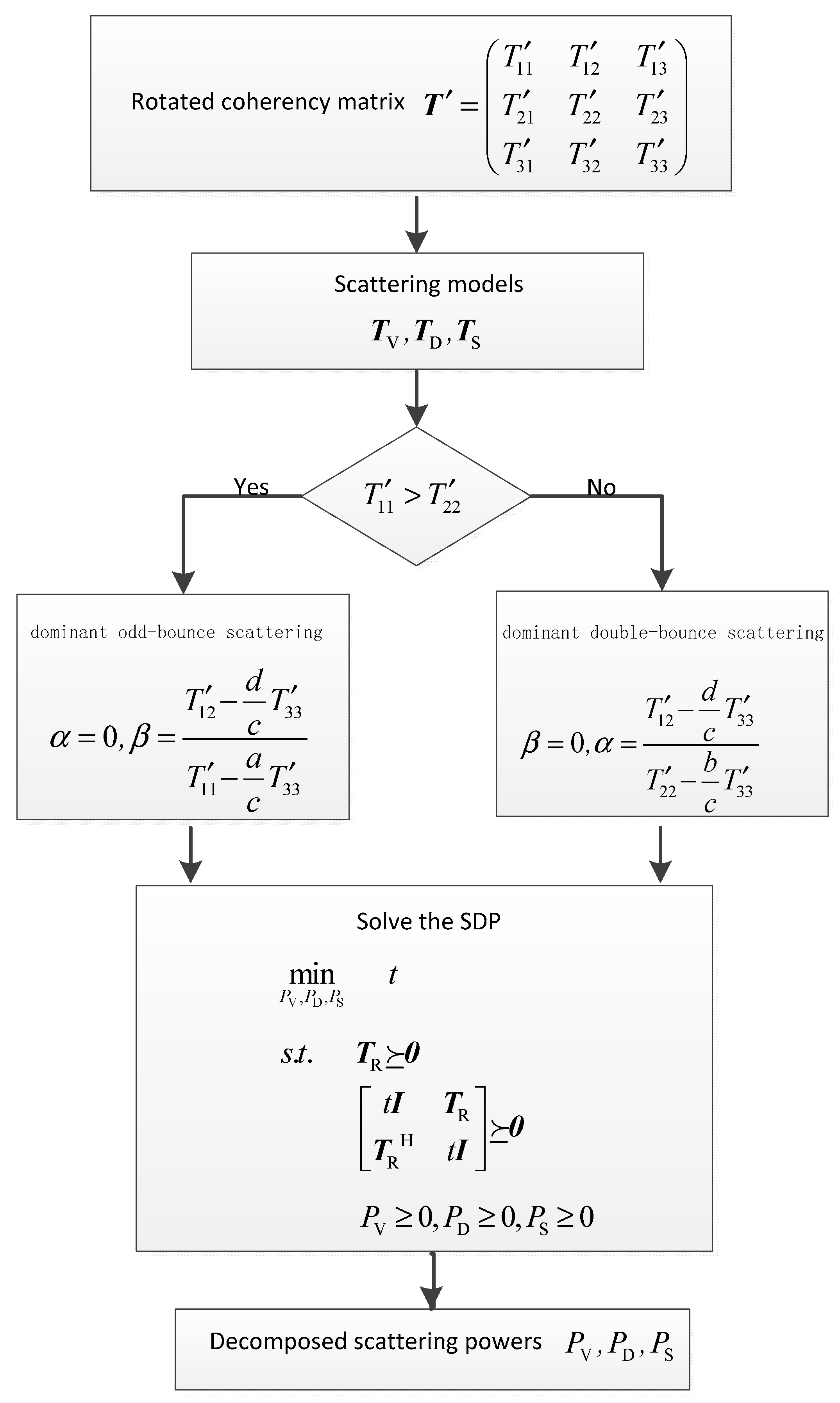
The detailed flowchart of the proposed decomposition process is shown in Figure 1.
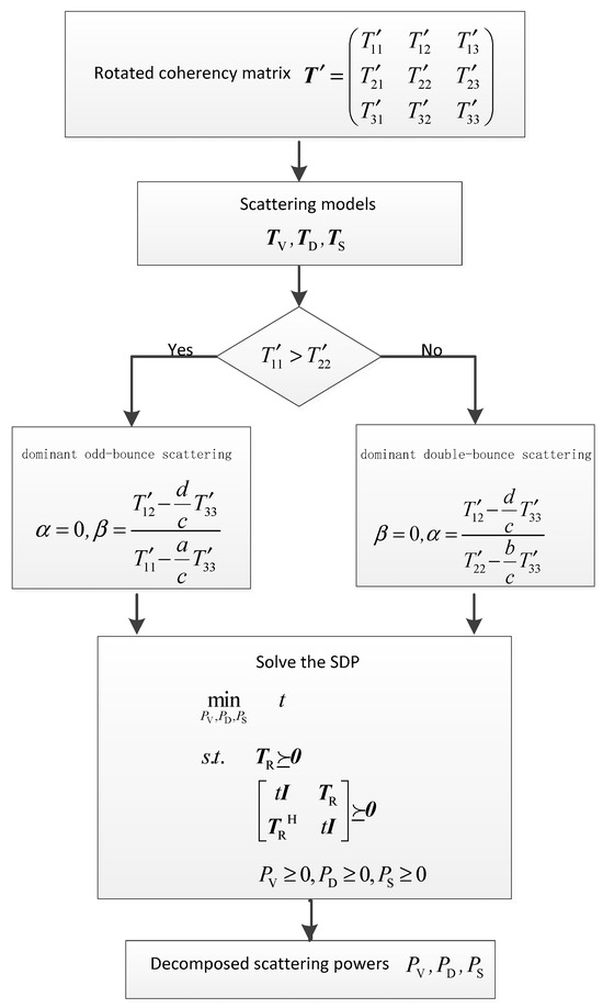
Figure 1.
Flowchart of the three-component polarimetric decomposition under the proposed method.
From the above, it can be seen that this article can globally optimize the energy of each scattering component. Compared with the commonly used method of remainder matrix Equation (17), this paper minimizes the remainder matrix based on the physical reality of nonnegative scattering components. Therefore, the residual of the proposed method is often higher than that of traditional methods. At the same time, this article only uses decomposition based on three basic models; the limited use of basic models cannot guarantee that the remainder matrix is zero after using the method proposed in this article. Additionally, the selection and accuracy of basic scattering models also have an impact on the residual.
5. Experimental Results and Analysis
To illustrate the proposed three-component decomposition method, comparison studies are carried out through the experiments on two different PolSAR data sets. Under the scattering symmetry assumption, comparing the result of proposed method with original FDD and NNED, meanwhile OAC method is used for comparison without the scattering symmetry assumption. The effectiveness of the proposed method can be analyzed from the following two aspects.
- (1)
- Ability to suppress the volume scattering power as well as the improvement of the double-bounce scattering and odd-bounce scattering.
- (2)
- Reduction in negative scattering power pixels, in fact, the proposed method avoids negative energy in principle.
5.1. AIRSAR L-Band PolSAR Data Set
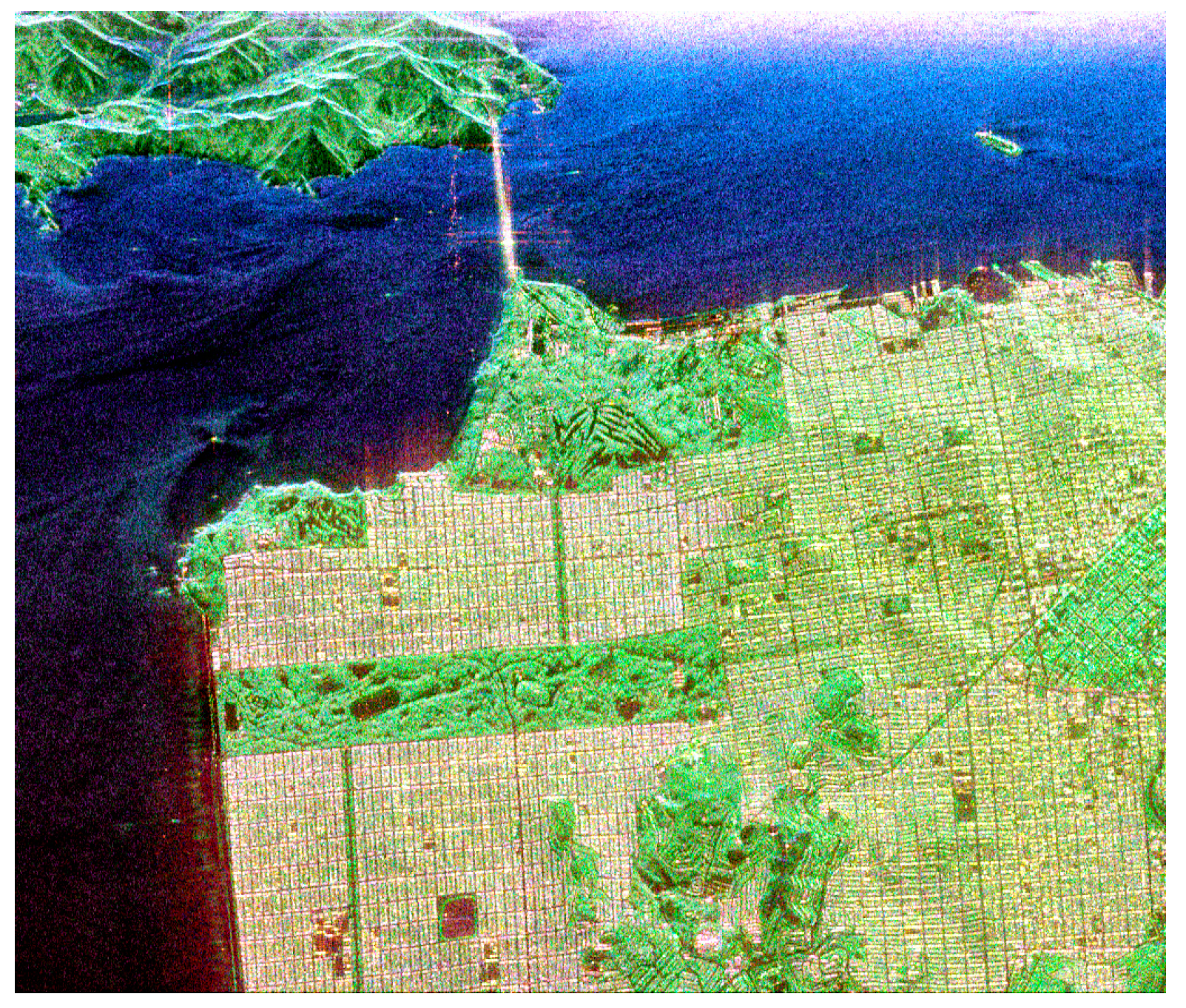
The proposed method is first validated on the AIRSAR L-band PolSAR data over San Francisco, as shown in Figure 2. This data was taken in 1994 at an angle of 5° to 60°, and the image has a dimension of pixels. The observed scene contains three main features, namely, ocean, urban area, and forest. To avoid the coupling of the speckle reduction, a specific speckle filter is not adopted.

Figure 2.
Pauli RGB image of the AIRSAR L-band San Francisco data set with different land-cover patches.
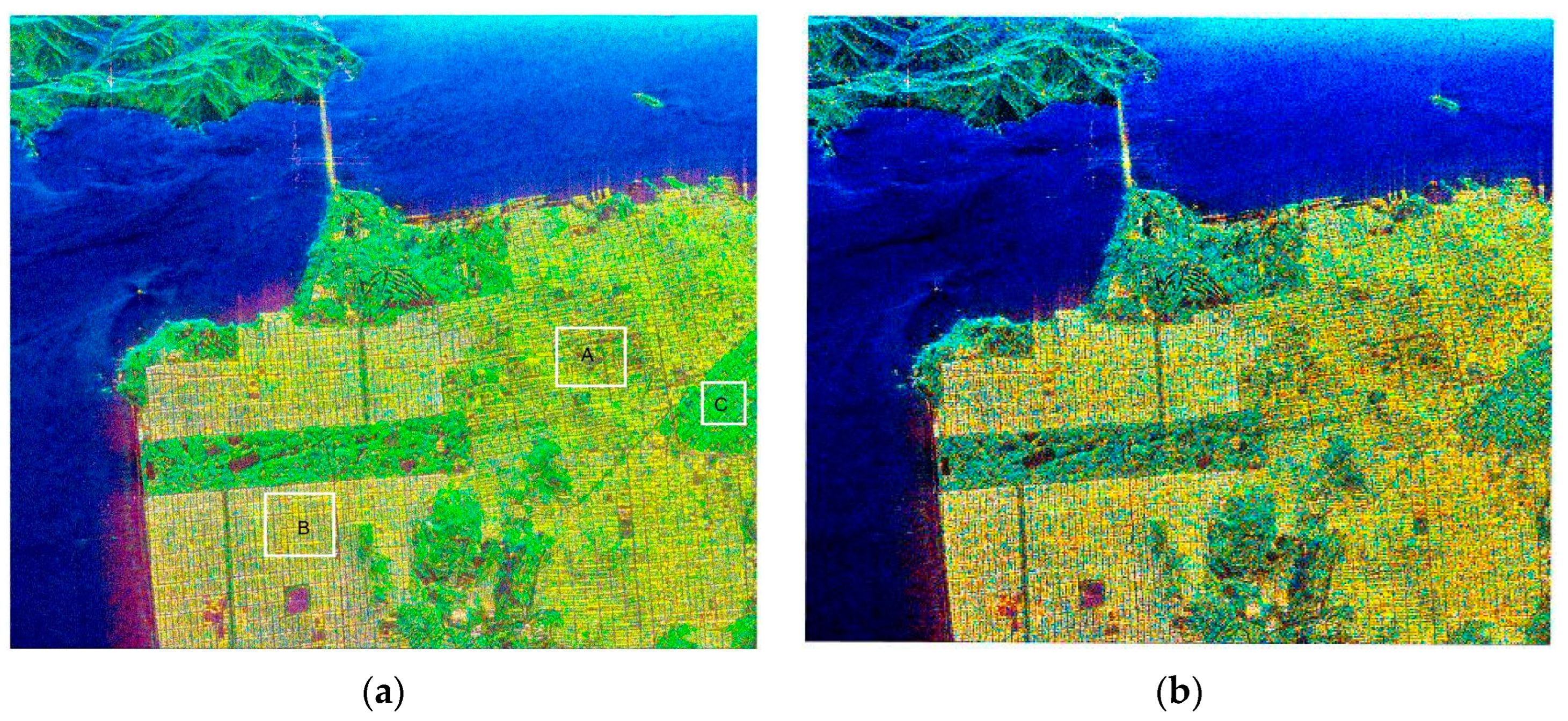
Under the scattering symmetry assumption, the decomposition results of FDD, NNED are shown in Figure 3a,b, respectively, whereas the decomposed image of the proposed method is shown in Figure 3c. Meanwhile, without the scattering symmetry assumption, the decomposed images of OAC and the proposed method are shown in Figure 4a,b. Patch A and B in Figure 3a are orthogonal urban areas, Patch C is highly oriented urban area. The OAC process is performed before the decomposition, which transforms the target orientation into a state of minimum cross-polarization power; therefore, the overestimation of volume scattering can be lessened slightly compared to FDD; the proposed three-component decomposition method obtains the global optimal results of scattering components by solving an SDP problem, which is described in Section 3 of this paper. In this demonstration, models of volume scattering , double-bounce scattering , and odd-bounce scattering adopt the models shown in Equations (5)–(7), and the relative strengths of the three scattering mechanisms are color-coded as red for double-bounce scattering contribution, green for volume scattering contribution, and blue for odd-bounce scattering contribution.
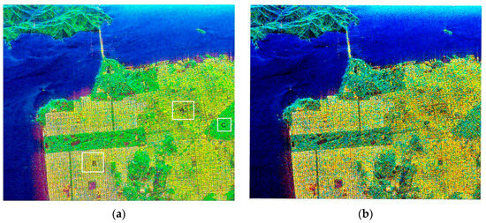
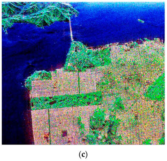
Figure 3.
Decomposition images of AIRSAR L-band San Francisco with scattering symmetry assumption. (a) FDD method. (b) NNED. (c) Proposed method. The images are colored by (green), (red), and (blue).
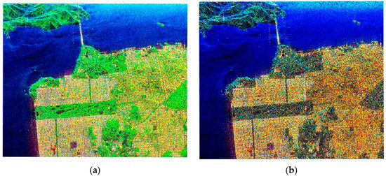
Figure 4.
Decomposition images of AIRSAR L-band San Francisco without scattering symmetry assumption. (a) OAC method. (b) Proposed method. The images are colored by (green), (red), and (blue).
For the analysis purpose, different patches are selected, as shown in Figure 3a. The quantitative comparison results of different regions are given in Table 1 and Table 2 in terms of the normalized mean of decomposed scattering powers. And the statistical results of negative scattering power pixels are shown in Table 3.

Table 1.
Normalized scattering contributions (%) of the selected patches with scattering symmetry assumption as defined in Figure 3a.
Table 2.
Normalized scattering contributions (%) of the selected patches without scattering symmetry assumption as defined in Figure 3a.
Table 3.
Percentage (%) of negative power pixels for AIRSAR L-band San Francisco image.
As shown in Figure 3, under the scattering symmetry assumption, the FDD, NNED, and the proposed decomposition method. On the whole, the ocean areas are odd-bounce scattering-dominant, the vegetation areas are dominated by volume scattering. The main difference among the three decomposition methods lies in built-up areas. The color contrasts appear strongest in built-up areas for the proposed decomposition method; this is mainly because the proposed decomposition method assigns less power to volume scattering than the FDD and NNED methods, as shown in Figure 3c. With establishing and solving the optimal problem of scattering mechanisms, improved performance is achieved especially in built-up areas. Without the scattering symmetry assumption case, the OAC method and the proposed decomposition method are compared, as shown in Figure 4. From Figure 4, it can be seen that the mountainous areas covered with forests are dominated by volume scattering, while built-up areas are dominated by double-bounce scattering. The main difference between Figure 4a and Figure 4b still lies in the oriented built-up areas. However, due to the assumption in conventional models that only the volume scattering contributes to the cross-polarization term, even with the OAC processing, the volume scattering may also be overestimated in built-up areas, as shown in Figure 4a. Figure 3c and Figure 4b show the results of the proposed decomposition method with and without the scattering symmetry assumption. Both Figure 3c and Figure 4b demonstrate the suppression ability of the proposed method for volume scattering overestimation; however, the difference between the two figures is mainly because the scattering mechanism energy in Figure 3c is not affected by the off-diagonal terms in the calculation process, so the coherency matrix can be more decomposed.
Table 1 and Table 2 analyze the relative contributions of the three scattering mechanisms; different land types are selected. Here, urban areas are given special attention (patches A and B), while urban with vegetation areas are also studied (patch C), as shown in Figure 3a. The results with and without the scattering symmetry assumption are tabulated in Table 1 and Table 2, respectively. As is discussed in [25], for FDD and OAC methods, only the pixels that yielded valid physical results were included in these weighted contributions.
Under the scattering symmetry assumption, as the normalized mean of decomposed scattering powers in Table 1, the proposed method further enhances the decomposition results by optimally solving the combination of scattering mechanisms. An additional increment of 3.39% by the proposed method of compared with FDD and 6% compared with NNED. For urban patch B, there is a similar result as for patch A, the proportion of by the proposed method has increased compared to the FDD and NNED methods. In the case of vegetation patch C, the contribution of the volume scattering component is 48.91% by the proposed method. As shown in Figure 3a, the selected vegetation area lies in the urban region and with large orientation angles; hence, this vegetation patch also expects significant odd and even-bounce scattering mechanisms.
For Table 2, in urban patch A, the streets are aligned in the radar line of sight direction; hence, the value of OAC in Table 2 is comparable to that of FDD in Table 1. Without the scattering symmetry assumption, the same conclusion can be drawn as for Table 1, that is, the proposed method can further increase the proportion of .
To check the physical reliability of the decomposed methods, the number of negative scattering power pixels is calculated for AIRSAR L-band San Francisco by different decomposition methods. In statistical analysis, only when the scattering mechanisms corresponding to each pixel are nonnegative can the pixel be considered nonnegative, and the result can be seen in Table 3. Model-based decomposition of FDD and OAC schemes computes the volume scattering power first. That is why the overestimation of volume scattering power is the main reason for leading the negative scattering pixels in model-based decomposition methods. Meanwhile, the NNED provided an algorithm from the perspective of eigenvalues that ensure the nonnegative power constraints; therefore, Table 3 does not consider the NNED method in negative scattering power pixels statistics. From Table 3, one can observe that FDD results in 72.10% negative power pixels. OAC reduced this amount to 57.78% by reducing volume scattering overestimation. However, the superiority of the proposed method can be observed, which has no negative value through the proposed optimization problem.
5.2. GaoFen-3(GF-3) C-Band PolSAR Data Set
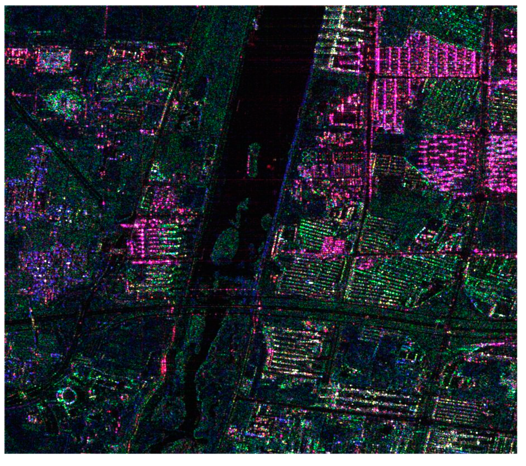
To further demonstrate the effectiveness of the proposed method, especially in the built-up areas. Analysis and comparisons are conducted with the PolSAR data set acquired by GF-3. The test site area mainly comprised a number of built-up patches, while the middle shows river cover; the image is shown in Figure 5.
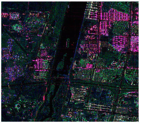
Figure 5.
Pauli RGB image of the GF-3 C-band PolSAR data set.
The decomposed images of the test site by FDD, NNED, and the proposed method under the scattering symmetry assumption are shown in Figure 6a–c, while decomposed images by OAC and the proposed method without the scattering symmetry assumption are shown in Figure 7a,b. Patch A and B in Figure 6a are urban areas. In this demonstration, models of volume scattering , double-bounce scattering , and odd-bounce scattering adopt the models shown in Equations (5)–(7); the relative strengths of the three scattering mechanisms are color-coded as the data set of AIRSAR L-band San Francisco. For analysis purposes, patches are selected as shown in Figure 7a; meanwhile, the percentage of the normalized mean of scattering powers by different methods and the number of negative scattering power pixels are calculated in Table 4, Table 5 and Table 6.
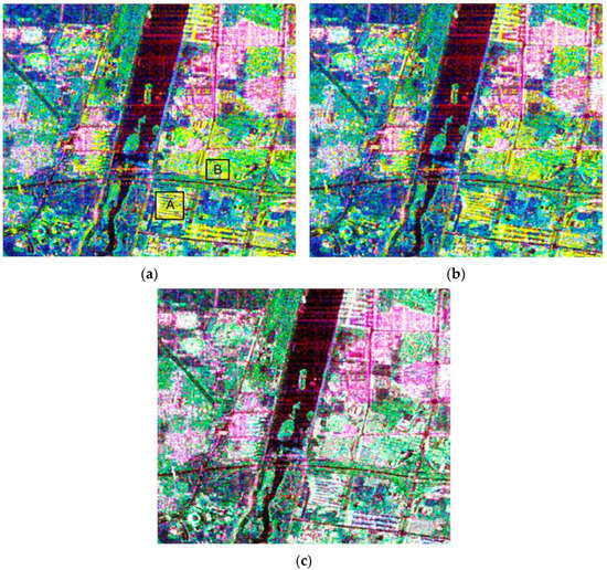
Figure 6.
Decomposition images of GF-3 C-band with scattering symmetry assumption. (a) FDD method. (b) NNED. (c) Proposed method.

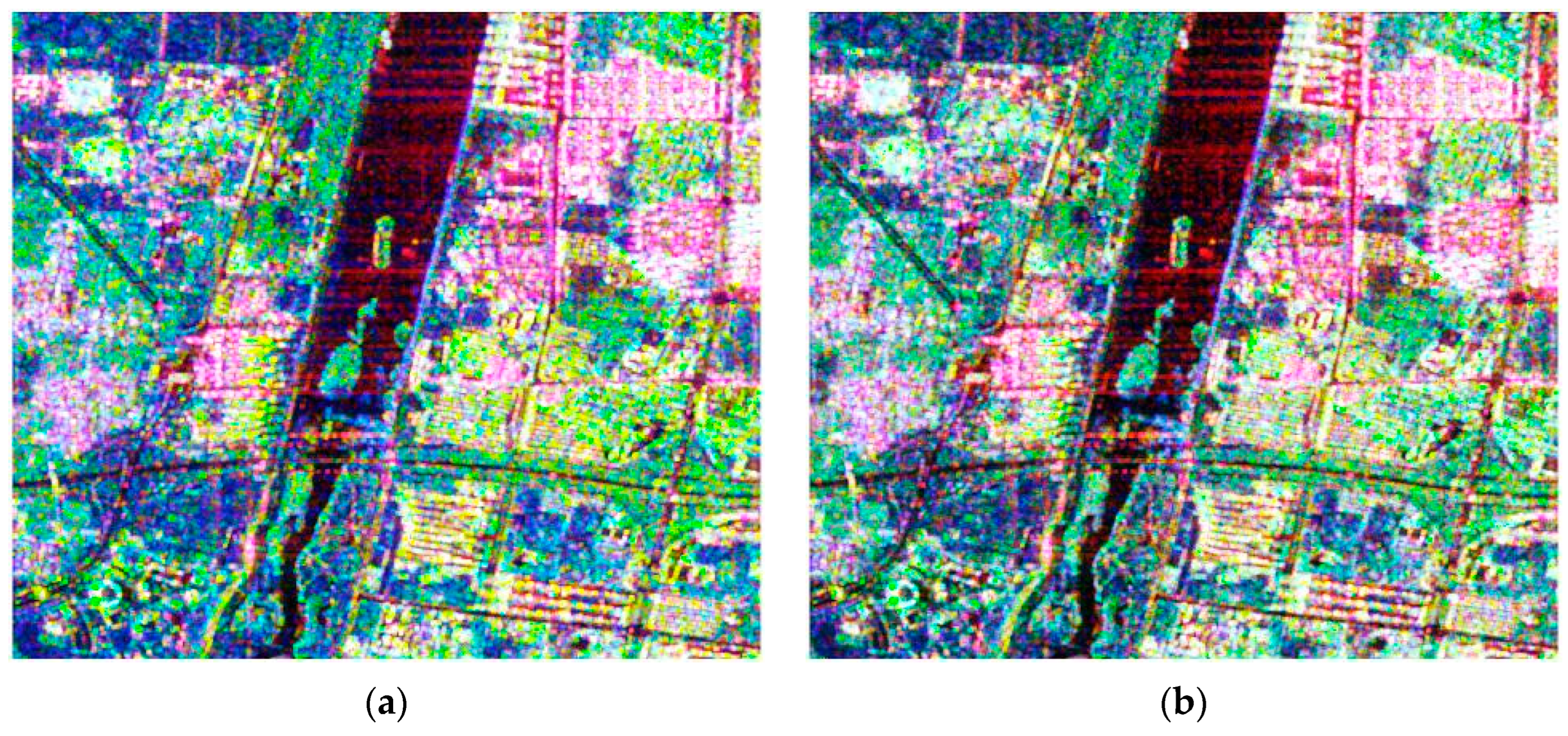
Figure 7.
Decomposition images of GF-3 C-band without scattering symmetry assumption. (a) OAC method. (b) Proposed method.
Table 4.
Normalized scattering contributions (%) of the selected patches with scattering symmetry assumption as defined in Figure 6a.
Table 5.
Normalized scattering contributions (%) of the selected patches without scattering symmetry assumption as defined in Figure 6a.
Table 6.
Percentage (%) of negative power pixels for GF-3 C-band o image.
From the decomposition results of FDD, NNED, shown in Figure 6a,b, the built-up areas do not reflect the dominance of double-bounce scattering and the misinterpretation is serious. With the global solving as proposed in this paper, the odd-bounce scattering contributions are obviously increased, shown in Figure 6c. Meanwhile, when the coherency matrix without the constraint of scattering symmetry assumption, by the deorientation processing, the volume scattering contribution can reduce, as shown in Figure 7a. However, the scheme computes the volume scattering power first, which still leads to the problem of overestimating volume scattering contribution. Further improved performance is achieved by the proposed decomposition method, shown in Figure 7b. The main difference between Figure 7a and Figure 7b still lies in the built-up areas. Both Figure 6c and Figure 7b demonstrate the suppression ability of the proposed method for volume scattering overestimation.
Table 4 and Table 5 are results of the percentage of the normalized mean of scattering powers by different methods with and without the scattering symmetry assumption. In the two tables, two patches are selected to be analyzed as shown in Figure 6a. From Table 4, which is the results with the constraint of the scattering symmetry assumption, one can see that the performance of the proposed method is better than FDD and NNED for both built-up patches. It is particularly noteworthy that the volume scattering power by the proposed method is 23.69% less than the of FDD method, while the double-bounce scattering power by the proposed method increases about 13%. As for the results without the constraint of the scattering symmetry assumption, shown in Table 5, the same conclusion can be drawn as for Table 4, that is, the proposed method can have less volume scattering power and can further increase the proportion of .
The number of negative power pixels by different decomposition methods for GF-3 C-band is calculated in Table 6. The calculation method is the same as the analysis of the AIRSAR L-band PolSAR data set, that is, only when the scattering mechanisms corresponding to each pixel are nonnegative can the pixel be considered nonnegative. The NNED method is a nonnegative decomposition method; therefore, it is not counted in Table 6. The percentage of negative power pixels for FDD and OAC methods are 20.95% and 12.77%, where the percentage of negative power pixels is 0% by the proposed method. This significant decrement is because the established optimization problem in this paper limits the generation of negative powers.
The optimization solution method proposed in this article is essentially the solution of nonlinear equations. Compared with linear solution methods such as FDD, any type of nonlinear optimization solution is inefficient or even ineffective in terms of time complexity. Although this article equivalently transforms the proposed optimization problem into an SDP problem that can be solved using the convex optimization toolbox SeDuMi, SeDuMi still involves a large number of function calls in the calculation process, and the complexity of model parameters directly affects the computational efficiency. This makes the method proposed in this article less advantageous in time complexity compared to linear solving methods. In the above experiment, local PC that configured the CPU of Intel Core i7, 16G memory was used to process the GF-3 data set, the FDD after the OAC method using linear operations had a processing time of approximately 25 s, while the proposed method using SeDUMi had a processing time of 430 times that of the FDD method. However, the method proposed in this article avoids the reflection symmetry assumption, and the branch conditions. In addition, it also avoids the problem of overestimating volume scattering and negative energy generation caused by traditional step-by-step solving methods, and provides a way for globally optimizing the parameters of the PolSAR model decomposition.
6. Conclusions
Model-based decomposition is the interpretation of radar backscatter by linear combination of basic scattering mechanisms. Physically, all scattering mechanisms must have nonnegative powers, and the remainder matrix after subtracting any linear combination of scattering mechanisms from the total backscatter should also have nonnegative eigenvalues.
In this paper, a global optimal model decomposition method based on the remainder matrix is proposed to optimize the fully PolSAR coherency matrix. The optimization is achieved by solving the problem using SDP based on the Schur complement theory. The method minimizes the maximum eigenvalue of the remainder matrix without the constraint of the scattering symmetry assumption. All the elements of the coherency matrix are taken into consideration in PolSAR processing and this method takes equal and unified consideration in analyzing each essential scattering component without the division of priority. The volume scattering overestimation is avoided, which appears frequently in the traditional decomposition method. Considering the physical reality that the power of each scattering term is nonnegative and the energy of the remainder matrix is nonnegative, the improved decomposition method makes non-negative as a constraint, which is more consistent with the actual distribution of the observed scene. Finally, the effectiveness of the proposed method is investigated by the AIRSAR L-band PolSAR and GF-3 C-band data sets; results show that the proposed method weakened the volume scattering power in comparison to FDD, NNED, and OAC. In addition, the negative power pixel count is also found to be significantly decreased to 0 by the proposed approach. The aforementioned make the proposed approach distinct and more suitable for the actual physical situation in comparison to the other relevant decomposition literature. Subsequent investigations will focus on the selection of volume scattering models for different scenarios and the influence of off-diagonal terms on PolSAR decomposition.
Author Contributions
Conceptualization, T.W. and Z.S.; methodology, T.W.; validation, T.W., Z.S. and P.J.; formal analysis, J.T.; investigation, Z.D. and T.Q.; resources, Z.S.; data curation, Z.S.; writing—original draft preparation, T.W.; writing—review and editing, Z.S.; visualization, Z.D. and J.T.; supervision, P.J. All authors have read and agreed to the published version of the manuscript.
Funding
This research received no external funding.
Data Availability Statement
Not applicable.
Acknowledgments
We thank the anonymous reviewers for their valuable comments to improve the paper’s quality.
Conflicts of Interest
The authors declare no conflict of interest.
Appendix A
The Schur complement is defined as follows [39].
Definition 1 (Schur Complement): Let be any Hermitian matrix of the form
where is the Hermitian matrix; suppose is invertible, that is . Then the matrix is called the Schur complement of in , and is satisfied.
With the above-mentioned definition, the following two lemmas will state that optimization problems Equations (15) and (16) are equivalent.
References
- Chen, S.; Li, Y.; Wang, X.; Xiao, S.; Sato, M. Modeling and interpretation of scattering mechanisms in polarimetric synthetic aperture radar: Advances and perspectives. IEEE Signal Process. Mag. 2014, 31, 79–89. [Google Scholar] [CrossRef]
- Wang, N.; Shi, G.; Liu, L.; Zhao, L.; Kuang, G. Polarimetric SAR target detection using the reflection symmetry. IEEE Geosci. Remote Sens. Lett. 2012, 9, 1104–1108. [Google Scholar] [CrossRef]
- Marino, A. A notch filter for ship detection with polarimetric SAR data. IEEE J. Sel. Top. Appl. Earth Obs. Remote Sens. 2013, 6, 1219–1232. [Google Scholar] [CrossRef]
- Yamaguchi, Y.; Sato, A.; Boerner, W.M. Four-component scattering power decomposition with rotation of coherency matrix. IEEE Trans. Geosci. Remote Sens. 2011, 49, 2251–2258. [Google Scholar] [CrossRef]
- Xi, Y.; Lang, H.; Tao, Y.; Huang, L.; Pei, Z. Four-component model-based decomposition for ship targets using polsar data. Remote Sens. 2017, 9, 621. [Google Scholar] [CrossRef]
- Krogager, E. New decomposition of the radar target scattering matrix. Electron. Lett. 1990, 26, 1525–1527. [Google Scholar] [CrossRef]
- Cameron, W.L.; Leung, L.K. Feature motivated polarization scattering matrix decomposition. In Proceedings of the IEEE International Conference on Radar, Arlington, VA, USA, 7–10 May 1990; pp. 549–557. [Google Scholar]
- Cameron, W.L.; Rais, H. Conservative polarimetric scatterers and their role in incorrect extensions of the cameron decomposition. IEEE Trans. Geosci. Remote Sens. 2006, 44, 3506–3516. [Google Scholar] [CrossRef]
- Cameron, W.L.; Rais, H. Derivation of a signed cameron decomposition asymmetry parameter and relationship of cameron to huynen decomposition parameters. IEEE Trans. Geosci. Remote Sens. 2011, 49, 1677–1688. [Google Scholar] [CrossRef]
- Cameron, W.L.; Rais, H. Polarization scatterer feature metric space. IEEE Trans. Geosci. Remote Sens. 2013, 51, 3638–3647. [Google Scholar] [CrossRef]
- Cloude, S.R.; Pottier, E. An entropy based classification scheme for land applications of polarimetric SAR. IEEE Trans. Geosci. Remote Sens. 1997, 35, 68–78. [Google Scholar] [CrossRef]
- Freeman, A.; Durden, S.L. A three-component scattering model for polarimetric SAR data. IEEE Trans. Geosci. Remote Sens. 1998, 36, 963–973. [Google Scholar] [CrossRef]
- Maurya, H.; Panigrahi, R. PolSAR coherency matrix optimization through selective unitary rotations for model-based decomposition scheme. IEEE Geosci. Remote Sens. Lett. 2019, 16, 658–662. [Google Scholar] [CrossRef]
- An, W.; Lin, M. A reflection symmetry approximation of multilook polarimetric sar data and its application to freeman–durden decomposition. IEEE Trans. Geosci. Remote Sens. 2019, 57, 3649–3660. [Google Scholar] [CrossRef]
- Maurya, H.; Bhattacharya, A.; Mishra, A.; Panigrahi, R. Hybrid three-component scattering power characterization from polarimetric sar data isolating dominant scattering mechanisms. IEEE Trans. Geosci. Remote Sens. 2022, 60, 1–15. [Google Scholar] [CrossRef]
- Yamaguchi, Y.; Moriyama, T.; Ishido, M. Four-component scattering model for polarimetric SAR image decomposition. IEEE Trans. Geosci. Remote Sens. 2005, 43, 1699–1706. [Google Scholar] [CrossRef]
- Yamaguchi, Y.; Yajima, Y.; Yamada, H. A four-component decomposition of POLSAR images based on the coherency matrix. IEEE Geosci. Remote Sens. Lett. 2006, 3, 292–296. [Google Scholar] [CrossRef]
- Cloude, S.R.; Pottier, E. A review of target decomposition theorems in radar polarimetry. IEEE Trans. Geosci. Remote Sens. 1996, 34, 498–518. [Google Scholar] [CrossRef]
- Chen, J.; Chen, Y.; Yang, J. Ship detection using polarization cross-entropy. IEEE Geosci. Remote Sens. Lett. 2009, 6, 723–727. [Google Scholar] [CrossRef]
- An, W.; Lin, M. Generalized Polarimetric Entropy: Polarimetric Information Quantitative Analyses of Model-Based Incoherent Polarimetric Decomposition. IEEE Trans. Geosci. Remote Sens. 2021, 59, 2041–2057. [Google Scholar] [CrossRef]
- Wang, Y.; Yu, W.; Liu, X. Demonstration and analysis of an extended adaptive general four-component decomposition. IEEE J. Sel. Top. Appl. Earth Obs. Remote Sens. 2020, 13, 2573–2586. [Google Scholar] [CrossRef]
- Xu, F.; Jin, Y.-Q. Deorientation theory of polarimetric scattering targets and application to terrain surface classification. IEEE Trans. Geosci. Remote Sens. 2005, 43, 2351–2364. [Google Scholar]
- Gulab, S.; Malik, R.; Mohanty, S. Seven component scattering power decomposition of POLSAR coherency matrix. IEEE Trans. Geosci. Remote Sens. 2019, 57, 8371–8382. [Google Scholar]
- Kusano, S.; Takahashi, K.; Sato, M. Volume scattering power constraint based on the principal minors of the coherency matrix. IEEE Geosci. Remote Sens. Lett. 2014, 11, 361–365. [Google Scholar] [CrossRef]
- Van Zyl, J.J.; Arii, M.; Kim, Y. Model-based decomposition of polarimetric SAR covariance matrices constrained for nonnegative eigenvalues. IEEE Trans. Geosci. Remote Sens. 2011, 49, 3452–3459. [Google Scholar] [CrossRef]
- Lee, J.S.; Ainsworth, T.L.; Wang, Y. Generalized polarimetric model-based decompositions using incoherent scattering models. IEEE Trans. Geosci. Remote Sens. 2014, 52, 2474–2491. [Google Scholar] [CrossRef]
- Lim, Y.X.; Burgin, M.S.; Van Zyl, J.J. An optimal nonnegative eigenvalue decomposition for the freeman and durden three-component scattering model. IEEE Trans. Geosci. Remote Sens. 2017, 55, 2167–2176. [Google Scholar] [CrossRef]
- Arii, M.; Van Zyl, J.J.; Kim, Y. Adaptive model-based decomposition of polarimetric SAR covariance matrices. IEEE Trans. Geosci. Remote Sens. 2011, 49, 1104–1113. [Google Scholar] [CrossRef]
- An, W.; Cui, Y.; Yang, J. Three-component model-based decomposition for polarimetric SAR data. IEEE Trans. Geosci. Remote Sens. 2010, 48, 2732–2739. [Google Scholar]
- Neumann, M.; Ferro-Famil, L.; Reigber, A. Estimation of forest structure, ground, and canopy layer characteristics from multibaseline polarimetric interferometric SAR data. IEEE Trans. Geosci. Remote Sens. 2010, 48, 1086–1104. [Google Scholar] [CrossRef]
- Arii, M.; Van Zyl, J.J.; Kim, Y. A general characterization for polarimetric scattering from vegetation canopies. IEEE Trans. Geosci. Remote Sens. 2010, 48, 3349–3357. [Google Scholar] [CrossRef]
- Hajnsek, I.; Jagdhuber, T.; Schon, H. Potential of estimating soil moisture under vegetation cover by means of PolSAR. IEEE Trans. Geosci. Remote Sens. 2009, 47, 442–454. [Google Scholar] [CrossRef]
- Chen, S.; Wang, X.; Xiao, S. General polarimetric model-based decomposition for coherency matrix. IEEE Trans. Geosci. Remote Sens. 2014, 52, 1843–1855. [Google Scholar] [CrossRef]
- Xie, Q.; Zhu, J.; Lopez-Sanchez, J.M.; Wang, C.; Fu, H. A Modified General Polarimetric Model-Based Decomposition Method with the Simplified Neumann Volume Scattering Model. IEEE Trans. Geosci. Remote Sens. 2018, 15, 1229–1233. [Google Scholar] [CrossRef]
- Xiang, D.; Wang, W.; Tang, T.; Su, Y. Multiple-component polarimetric decomposition with new volume scattering models for PolSAR urban areas. IET Radar Sonar Navig. 2017, 11, 410–419. [Google Scholar] [CrossRef]
- Li, D.; Zhang, Y.; Liang, L. A Mathematical Extension to the General Four-Component Scattering Power Decomposition with Unitary Transformation of Coherency Matrix. IEEE Trans. Geosci. Remote Sens. 2020, 58, 7772–7789. [Google Scholar] [CrossRef]
- Xiao, J.; Nehorai, A. Joint Transmitter and Receiver Polarization Optimization for Scattering Estimation in Clutter. IEEE Trans. Signal Process. 2009, 57, 4142–4147. [Google Scholar] [CrossRef]
- Sturm, J.F. Using SeDuMi 1.02, a MATLAB toolbox for optimization over symmetric cones. Optim. Methods Software. 1999, 11, 625–653. [Google Scholar] [CrossRef]
- Horn, R.; Johnson, C. Matrix Analysis; Cambridge Univ. Press: New York, NY, USA, 1986; Chapter 7. [Google Scholar]


Disclaimer/Publisher’s Note: The statements, opinions and data contained in all publications are solely those of the individual author(s) and contributor(s) and not of MDPI and/or the editor(s). MDPI and/or the editor(s) disclaim responsibility for any injury to people or property resulting from any ideas, methods, instructions or products referred to in the content. |
© 2023 by the authors. Licensee MDPI, Basel, Switzerland. This article is an open access article distributed under the terms and conditions of the Creative Commons Attribution (CC BY) license (https://creativecommons.org/licenses/by/4.0/).