Studying Conditions of Intense Harmful Algal Blooms Based on Long-Term Satellite Data

Abstract

Harmful algal blooms (HABs) adversely impact aquatic organisms, human health, and the marine economy. The need to understand the origins and mechanisms of HAB occurrence and development determines the relevance of the study of these phenomena, including using remote sensing methods and assets. Here we present the results of a comprehensive study of conditions and precursors of some intense HABs detected in the water areas near the island of Chiloe (Chile, 2016), near the Kamchatka Peninsula (Russia, 2020), near the island of Hokkaido (Japan, 2021), among others. The study involves statistical analysis of long-term satellite and model data arrays on significant parameters of the marine environment and near-surface atmosphere, as well as empirical modeling of HAB risks. Information products on the following environmental parameters were used: sea surface temperature (SST, NOAA OISST, since 1981), the level of photosynthetically active radiation (PAR) and chlorophyll-a concentration (MODIS Ocean Color SMI, since 2000), sea surface salinity and height (HYCOM, since 1993), and near-surface wind speed and direction (NCEP CFSv2, since 1979). Quantitative assessments of the dynamics of informative criteria were applied. The key criterion is the ratio (${\mathsf{\Delta }}_{\mathsf{\sigma }}$) of the absolute deviation of the studied parameter from the expected norm to the RMS deviation of its values. Intense HABs were often preceded by excessive SST (up to ${\mathsf{\Delta }}_{\mathsf{\sigma }}$ ~1.99) and PAR (up to ${\mathsf{\Delta }}_{\mathsf{\sigma }}$ ~2.25) values, as well as low near-surface wind speed (up to ${\mathsf{\Delta }}_{\mathsf{\sigma }}$ ~−1.83). These environmental parameters considerably contribute to HAB generation and intensification. An approach and empirical function were proposed that allow us to assess the risk of HAB phenomena and reveal their precursors. Using the proposed approach and empirical function, the precursors of ten HABs were identified, nine of which were confirmed by in situ data. The results can be used as a tool for forecasting and studying the conditions for the occurrence of HABs, representing one of the promising directions for monitoring these dangerous phenomena.

1. Introduction

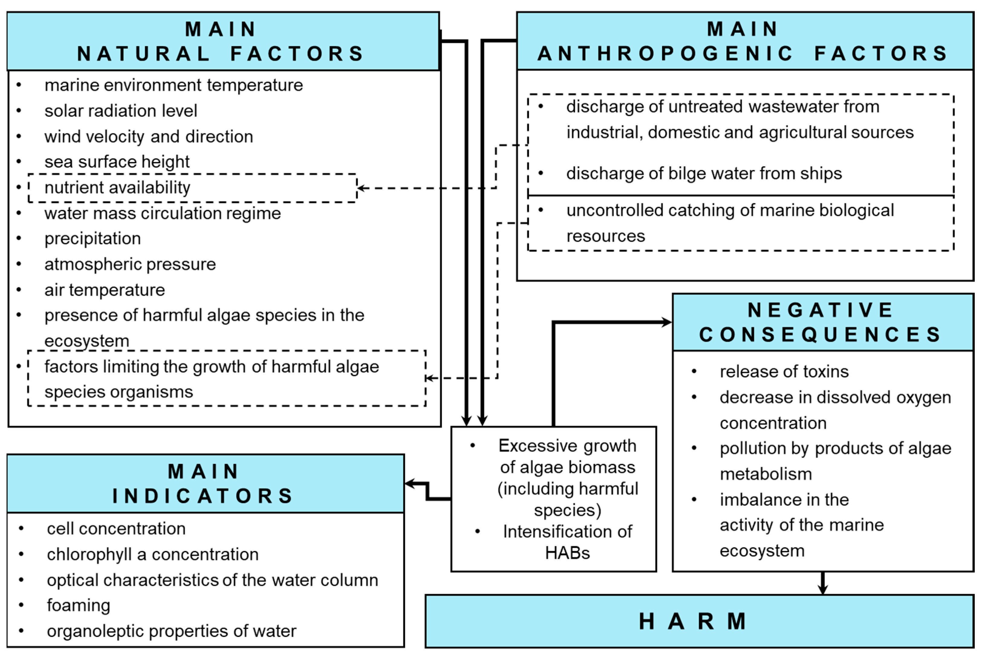
1.1. HAB Issues and Some of the Most Intense Cases

Harmful algal blooms (HABs) are one of the specific processes occurring in marine ecosystems. Their consequences have serious negative impacts on aquatic organisms and humans, in addition to limiting the use of fish resources and reducing the recreational potential of coastal areas [1,2]. Over the past few years, a number of intense HABs have been registered in various areas of the World Ocean. The following three cases can be distinguished among the most extreme HABs:

• Harmful algal blooms (genus Pseudochattonella and genus Alexandrium) in the bays of Ancud and Corcovado out of the island of Chiloe (Chile), occurred in February–March 2016 [3]. Mass commercial fish mortality (Atlantic salmon, Coho salmon, and trout) was recorded, which led to a large economic loss (about USD 800 million) [4].
• Harmful algal bloom (genus Karenia and genus Pseudo-nitzschia) in Avacha Bay out of the Kamchatka Peninsula (Russia) in September–October 2020 [5,6,7]. The main consequences of this HAB were the mass killing of hydrobionts, the deterioration of people’s health, and intensive foaming on the coastline [5,6,8].
• Harmful algal bloom (genus Karenia) in the waters out of the island of Hokkaido (Japan) and the Southern Kuril Islands (Russia) in September 2021, resulting in the deaths of a large number of sea urchins and salmon, as well as general damage to coastal ecosystems [9].

1.2. Summarized HAB Research Approaches

Currently, detailed studies of such phenomena are carried out through both ground-based and remote measurements. Modern satellite remote sensing systems are characterized by a number of advantages that are important for the research of HABs in marine areas. These advantages include, among others, wide coverage; operational efficiency; exploration of hard-to-reach ocean areas; different spatial and temporal resolution of data collected in different parts of the electromagnetic spectrum; registration of a wide range of significant parameters of the aquatic environment; high reliability of the information received, etc. [10]. As the most important feature of satellite data and crucial for this study, the regularity of satellite data and a long retrospective of accumulated archives should be noted (for example, NOAA OISST satellite sea surface temperature, since 1981). The effectiveness of satellite remote sensing methods for detecting and investigating natural and anthropogenic impacts on the aquatic environment increases greatly when they are combined with the results of in situ measurements [11,12] and modeling [13,14,15,16,17].

Optical methods of satellite monitoring have some disadvantages, i.e., dependence on illumination conditions and clouds, and the need for atmospheric correction and calibration. However, such methods provide ample opportunities for the study of various anomalous processes in the seas and oceans, including intense HABs [18,19,20,21,22,23].

One of the areas of HAB research involves the interpretation of bloom indicators and the use of algae recognition algorithms based on satellite data [22]. Another area is the assessment of the biophysical relationships between different types of phytoplankton and the characteristics of the aquatic environment. Factors that potentially cause the growth of a particular type of algae can be considered [24]. Furthermore, HAB conditions and development features can be studied based on time series of well-proven standard informational products of satellite oceanography [23]. For example, in [4,8,17,23,25,26], increased temperatures of the marine environment and the level of PAR recorded by satellite methods were considered factors that had a key influence on the recorded cases of HABs.

1.3. The Purpose and Key Directions of the Research

The purpose of this study is to analyze long-term time series of satellite and model data on the natural conditions of the environment where the three above-mentioned intense HABs occurred (off the island of Chiloe (Chile), adjacent to the Kamchatka Peninsula (Russia), and off the island of Hokkaido (Japan)), in the interest of the following:

(1)

identification and interpretation of the dynamics of significant parameters of the marine environment and the near-surface layer of the atmosphere (hereinafter, investigated parameters, significant environmental parameters) before those HABs;

(2)

the capability to determine HAB risk levels by analyzing the time series of the significant environmental parameters.

The present work operates with an array of long-term series of heterogeneous satellite and model data on significant environmental parameters. Full algorithmic processing of such an array is carried out. Various types of informative criteria, which are important for the analysis of conditions for HAB occurrence, were calculated and analyzed based on the processing of these parameters. Furthermore, an approach and an empirical function to assess the HAB occurrence risk level are proposed in this effort. The results are expected to be significant and will contribute to further HAB research.

2. Materials and Methods

2.1. Prerequisites for the Research Approach

The development of HABs can be caused by many different factors, usually by their combined effect, which must be taken into account when selecting methods for their remote registration. To reveal such factors, we carried out a review of scientific papers devoted to the following:

• general features of HABs [2,27,28];
• types and degrees of damage resulting from intense HABs [2,28];
• factors affecting the occurrence of HABs and their subsequent development [29,30,31,32];
• features and indicators associated with HABs [33,34];
• various approaches to HAB studies [33,34,35,36];
• methods of remote registration of such anomalous phenomena [8,24,37,38].

Based on the analysis of the above publications, an integrated generalizing scheme was compiled containing some of the main factors and indicators directly accompanying HABs, as well as their negative consequences (Figure 1).

Figure 1 shows the main natural and anthropogenic factors that potentially affect the excessive growth of algae biomass and the intensification of the development of HABs (shown by the black arrows in Figure 1). Among the natural factors affecting the intensification of the development of HABs in marine ecosystems, the following can be distinguished (see Figure 1):

• marine environment temperature (see, for example, [8,23,39]);
• solar radiation level (see, for example, [19,40,41]);
• wind velocity and direction [26,42];
• sea surface height [25];
• water mass circulation mode, currents, internal waves [43,44,45];
• the presence of harmful algae species in the ecosystem [28];
• some meteorological parameters (precipitation, atmospheric pressure, and air temperature).

Natural factors in HABs’ intensification also include salinity. However, salinity has a bidirectional effect on microalgae. In some cases, salinity changes can stress the algae and cause them to release toxins. At the same time, some algae species tolerate salinity changes.

The following anthropogenic factors affecting HABs are important (see Figure 1):

• discharge of untreated wastewater from industrial, domestic, and agricultural sources [46];
• discharge of bilge water from ships, emergency and operational ship spills (see, for example, [47]).

The main indicators directly accompanying the HAB processes are as follows (see Figure 1):

• increased concentration of toxic and harmful algae cells [27,28];
• increased chlorophyll-a concentration [8,23,28];
• changes in optical characteristics of the water column [20,21];
• deterioration of organoleptic properties of water [5,28].

The main negative consequences of HABs (see Figure 1) leading to large-scale environmental and economic damage are as follows:

• release of toxins [28];
• decreased concentration of dissolved oxygen [28];
• pollution by algae metabolism products, an imbalance in the functioning of the marine ecosystem [48].

The impact of some natural factors is sometimes enhanced by the influence of anthropogenic ones. For example, the availability of nutrients can be increased due to the influx of excessive amounts of industrial biogenic elements into the water area [2]. Such a relationship is shown in Figure 1 by dashed arrows. Let us also note other unobvious factors influencing HABs. For example, an increase in nutrient content in the ocean and favorable conditions for HABs may occur due to the deposition of particles of various substances onto the sea surface as a result of sand and dust storms [49].

It should be noted that none of these factors alone, as a rule, cause a HAB. Studies of registered HAB cases usually indicate the combined action of several factors, and their specific composition depends on the physical and geographical characteristics of the water area, the level of anthropogenic load, the degree of dependence on climatic trends, etc. [32,49,50].

In this paper, a long-term series of satellite data on significant parameters of the marine environment and the near-surface layer of the atmosphere are used to investigate the potential relation of the studied HABs’ features with the dynamics of some of the mentioned factors.

2.2. Features of the Studied Water Areas

The marine areas where the studied specific events occurred (see Figure 2) were characterized by various conditions and historically were subjected to microalgae blooms of varying intensity and degree of harmful impact on marine waters.

The water area around Chiloe Island (see Figure 2A), covering mainly the zone between the island itself and the continent, is a semi-closed bay with depths of less than 300 m. This area is characterized by high spatial variability of oceanographic conditions as well as the presence of many fjords, channels, straits, and estuaries [51,52].

The water area off Avacha Bay near the Kamchatka Peninsula is open (see Figure 2B), which provides a relatively intensive water exchange with the Pacific Ocean. The depths of Avacha Bay vary from 40–60 m or less near the coast to 300–500 m on the shelf [53,54].

The water area off the island of Hokkaido (Figure 2C) covers coastal waters to the south and southeast of it, as well as waters adjacent to the southeastern coast of the Southern Kuril Islands. This studied water area is quite open to Pacific waters and is characterized by a wide range of depths, from 200 m in the coastal zone to 5000–6000 m in the oceanic basin. At the same time, it is worth noting that in the water area off Hokkaido Island, the coastline is slightly indented in comparison with other islands of the archipelago [55].

The main natural and climatic characteristics of the studied sites (first of all, temperature, hydrological regime, circulation of air masses, and amount of solar radiation) are different and variable, which will be seen below when presenting the materials of this study.

2.3. Used Data

The study of intensive HABs in these areas was carried out using remote sensing data by assessing the dynamics of significant parameters of the marine environment and the near-surface layer of the atmosphere (hereinafter, investigated parameters or significant environmental parameters). Both potential factors of HAB occurrence (temperature, level of photosynthetically active radiation, speed and direction of the near-surface wind, etc.) and indicators of HAB intensity (chlorophyll-a concentration, optical characteristics of the water column, etc.) were of interest for this study (see the diagram in Figure 1) [24,25,39]. In general, this effort focuses on the study of potential factors that contributed to the development of HABs.

For this purpose, long-term series of satellite and model data (including spatial distributions created on their basis) on the following parameters were used:

• sea surface temperature (SST) obtained on the basis of AVHRR satellite spectroradiometer data and NOAA OISST model data [56];
• the level of photosynthetically active radiation (PAR), calculated from MODIS (AQUA/TERRA satellites) spectroradiometer data [57,58];
• chlorophyll-a concentration (CHL-a), calculated from MODIS (AQUA/TERRA satellites) spectroradiometers [59,60];
• anomalies of the sea surface height (SSH), calculated using the HYCOM hybrid isopycnic ocean model [61];
• salinity of the water column at a depth of 0 m (sea surface salinity, SSS), calculated using the HYCOM hybrid isopycnic ocean model [61];
• latitudinal and meridional components of the near-surface wind vectors, calculated using the NCEP CFSv2 model [62].

A more detailed description of the data used in this study, their features, as well as data sources are given in

Table 1. Significant environmental parameters and their features, and data sources.

Parameter	Type of Relationship with HABs	Time Range	Time Interval of the Initial Data	Data Source
Sea surface temperature (SST)	Intensification factor	1 September 1981–31 December 2021	Daily	https://www.ncei.noaa.gov/products/climate-data-records/sea-surface-temperature-optimum-interpolation (accessed on 22 June 2023)
Photosynthetically active radiation (PAR)	Intensification factor	24 February 2000–31 December 2021	Monthly	https://oceancolor.gsfc.nasa.gov (accessed on 27 June 2023)
Chlorophyll-a concentration (CHL-a)	Indicator	24 February 2000–31 December 2021	Daily	https://oceancolor.gsfc.nasa.gov (accessed on 27 June 2023)
Sea surface salinity (SSS)	Intensification factor	2 October 1992–31 December 2021	Daily	https://hycom.org/ (accessed on 6 June 2023)
Anomaly of sea surface height (SSH)	Intensification factor	2 October 1992–31 December 2021	Daily	https://hycom.org/ (accessed on 6 June 2023)
Wind velocity (WV)	Intensification factor	1 January 1991–31 December 2021	4 times a day	https://www.cpc.ncep.noaa.gov/products/CFSv2/CFSv2_body.html (accessed on 28 June 2023)

.

During the process of obtaining information, the quality of the obtained initial data was monitored and the pixels of the land were excluded. The use of such a set of initial data is determined by the results of previous studies [5,8,19,23], since these data have found useful application in attempts to analyze the circumstances of the occurrence and development of HABs. Further in this article, the significance of these types of data for the study of the processes of HAB development will be investigated. The main limitations associated with the source data are various retrospective depths (see Table 1) and dependence on hydrometeorological conditions (which leads to spatial irregularity and empty pixels). These limitations are taken into account and correctly processed through the methods used in the work.

2.4. Methodology

2.4.1. An Approach to Informative Criteria Based on a Long-Term Series of Investigated Parameters

In the present study, based on the results of processing the long-term series of investigated parameters (P), given in Table 1, a time series of important informative criteria for the study of HABs has been formed. The following criteria were used:

• absolute deviation (${\mathsf{\Delta }}_{abs}$) of the investigated parameter from the expected level (see Equations (1) and (2));
• relative deviation (${\mathsf{\Delta }}_{rel}$) of the investigated parameter from the expected level (see Equation (3));
• the ratio of ${\mathsf{\Delta }}_{abs}$to σ, i.e., RMS spread of the investigated parameter (${\mathsf{\Delta }}_{\mathsf{\sigma }}$) (see Equations (4) and (5)).

In this effort, a regular time grid with an interval of 1 month was used. The expediency of using such a time grid was demonstrated earlier in [19].

The monthly mean values of each significant environmental parameter, P, for the current month are calculated using Equation (1). Equation (1) takes into account the uneven distribution of the number of observations within the studied water areas, caused, among other things, by the presence of clouds:

$$P_{month.mea{n}_m}=\frac{{{\displaystyle \sum }}_{j=1}^{n_m}{s}_{j,m}}{n_m}$$

(1)

where m is the end-to-end ordinal number of the month in a multi-year time series of observations (for example, for a ten-year time series, m will be from 1 to 120; the actual duration of the time series used is shown in Table 1); $n_m$ is the number of pixels within the studied water area, where at least one satellite measurement was taken during a given month; $s_{\mathrm{j},\mathrm{m}}$ is the monthly mean value of the studied parameter in the current pixel (j is the pixel number) within the studied water area for a given month.

The absolute deviation of the studied parameter from the expected level for each studied area was calculated as follows:

$${\mathsf{\Delta }}_{ab{s}_m }=P_{month.mea{n}_m}-\overline{P_{M,Y}}$$

(2)

where $\overline{P_{M,Y}}$ is the expected value of the parameter under study (the climatic norm, conditionally), corresponding to the current month, with the ordinal number M for year Y, calculated as the mathematical expectation of a number of monthly mean values in a given month M (takes on values from 1 to 12) of this parameter, registered within the boundaries of the processed area during all previous years.

The value ${\mathsf{\Delta }}_{ab{s}_m}$was often used in attempts to identify short-period anomalies of the studied parameters [5,8,63,64], but the informativeness of this criterion is limited. Therefore, this study also included criteria ${\mathsf{\Delta }}_{rel}$and${\mathsf{\Delta }}_{\mathsf{\sigma }}$ [19,65].

The relative deviation of the significant environmental parameter from the expected level for each water area was calculated as follows:

$${\mathsf{\Delta }}_{rel} {=\mathsf{\Delta }}_{ab{s}_m}/P_{month.mea{n}_m}·100\%$$

(3)

The root mean square spread of the investigated parameter values observed in the corresponding month M of year Y was calculated as follows:

$${\mathsf{\sigma } }_{M,Y} =\sqrt{\frac{\sum {\left(\left(P_{month.mea{n}_m}\right){ }_{Y }-({\overline{P_M)}}_Y\right)}^2}{N}}$$

(4)

where N is the number of years included in the analyzed time series before the current year.

The ratio of the absolute deviation of the current monthly mean value of the investigated parameter to the standard deviation of the values of this parameter was calculated as follows:

$${\mathsf{\Delta }}_{{\mathsf{\sigma }}_m}={\mathsf{\Delta }}_{ab{s}_m}/{ \mathsf{\sigma } }_{M,Y}$$

(5)

The described approach to the processing of long-term data series was applied for each of 6 types of investigated parameters given in Table 1 (SST, PAR, CHL-A, SSH, SSS, and WV), for each of the 3 studied water areas (18 datasets in total).

Informative criteria ${\mathsf{\Delta }}_{abs}$, ${\mathsf{\Delta }}_{rel}$, and ${\mathsf{\Delta }}_{\mathsf{\sigma }}$ were calculated for each of these 18 datasets using Equations (1)–(5). Such an operation was performed for each month from the beginning of the data archive (for example, for the SST, since 1981) and up to the year of registration of the studied intensive HAB (for example, for the area near Hokkaido Island, until 2021, inclusive). At the same time, a specially developed IDL program that provided cyclic (with a sequential increase in m, i.e., the end-to-end month number in a multi-year time series) calculation of results using Equations (1)–(5) and related service procedures was used. The use of cyclic calculations was necessary because, depending on the year number Y, values $\overline{P_{M,Y}}$ and${ \mathsf{\sigma } }_{M,Y}$ are gradually changing due to the addition of new elements to the data array. The results of the cyclic calculation for each of the 18 datasets were aggregated in the form of a multi-year time series of informative criteria ${\mathsf{\Delta }}_{ab{s}_m}$, ${\mathsf{\Delta }}_{re{l}_m}$, and ${\mathsf{\Delta }}_{{\mathsf{\sigma }}_m}$.

As additional informative criteria, long-term trends of the investigated parameters (linear regression slope coefficients) were calculated and analyzed, and historical maxima/minima of these parameters were recorded.

Thus, a retrospective array of informative criteria important for the study of the processes of HAB development was obtained, which was further analyzed in Section 3 of this article.

The process of informative criteria calculation as well as the quality of the initial data (no data gaps, no inadequate values, etc.) were controlled through the analysis of the long-term dynamics of the monthly mean values of all studied parameters for all months M for each of the studied water areas with superimposed ${\mathsf{\Delta }}_{ab{s}_m}$, ${\mathsf{\Delta }}_{re{l}_m}$, and ${\mathsf{\Delta }}_{{\mathsf{\sigma }}_m}\mathrm{graphs}$. A total of 216 such graphs were generated and analyzed (18 sets for each of the 12 months of the year). The adequacy of the calculations was validated based on the analysis of these graphs.

2.4.2. Experimental Function for Assessing the HAB Risk Level

Since the number of intense HABs in various areas of the World Ocean is increasing, the study of HAB risks and their forecast has become urgent. To solve this task, various approaches were used, as follows [66]:

• conceptual;
• empirical;
• numerical.

There are, for example, approaches to the detection and prediction of HABs proposed in [67,68,69,70,71], which are aimed at assessing the risk of the occurrence of algal blooms, as well as identifying the relationships of these processes with key physical and biological factors.

In this paper, we propose an empirical approach that allows us to register signals of increased probability of HABs. At the same time, it is assumed that the significant environmental parameters used (primarily sea surface temperature, photosynthetically active radiation, and near-surface wind velocity) have a complex effect on the ecosystem, and abnormal changes in these parameters can cause the development of intensive (including harmful) algal blooms. Numerous works cited above confirm this assumption. At the same time, the input data for assessing the risk of HABs are time series of informative criteria calculated as a result of processing long-term time series of the three key investigated parameters: SST, PAR, and WV.

Table 2. Rating of the significance of SST, PAR, and WV factors in studies of HABs based on the review [72].

Potential Impact on HAB Intensification	Rating of the Factor Significance in HAB Research	Number of Publications Identifying the Factor as Influencing HAB Intensification	The Nature of the Relationship between the Factor and Harmful Bloom
SST	3	39	Positive
PAR	2	9	Positive
WV	1	7	Negative

shows the rating of parameters that potentially influence the intensification of HABs. The rating is supported by information from the review in [72], which is also shown in Table 2: the number of publications devoted to each of these factors and the nature of the relationship between these factors and HABs.

We also assume that the effect contributing to the occurrence and intensification of HABs accumulates over a period of time. Therefore, the proposed function for calculating the HAB risk $\overline{R}$for the time interval m is given as the sum of several values of the conditional value r (conventionally called the “integrated HAB-risk factor”), which are accumulated over a certain number of time grid intervals.

With this in mind,

$$\overline{R_m}={{\displaystyle \sum }}_{z=m - \mathsf{\delta }}^{m - 1 }{r}_z$$

(6)

where $r_z$is the integrated HAB risk factor, calculated by several significant environmental parameters under study, upon the occurrence of the z-th ordinal time interval in the range z from m − δ to m − 1; δ is the number of time intervals used for signal accumulation (if δ = 1, 1 accumulation interval “m − 1” is used). In this study, it was assumed that the value of $\overline{ R_m }$ (6) is proportional to the risk of HABs. This assumption was tested during computational experiments and the analysis of their results.

The complex risk factor r for the time interval z can be estimated using the following equation:

$${\mathrm{r}}_{\mathrm{z}}=k_{\mathrm{z}}{{\displaystyle \sum }}_{j=1}^n\left({\mathsf{\Delta }}_{{\mathsf{\sigma }}_{z,j}}+F_{z,j}\right)v_j$$

(7)

where n is the number of investigated parameters used (j is the ordinal number of the parameter); ${\mathsf{\Delta }}_{{\mathsf{\sigma }}_{z,j}}$is the ratio of deviations of the actual values of the j-th parameter from the expected level to their standard deviation for the z-th time interval (see Equation (5)); $F_{z,j}$ is an addend that takes into account an additional HAB risk factor associated with the j-th parameter in the z-th time interval; $v_j$ is the coefficient that balances the significance of each of the n investigated parameters, in addition to determining the nature of the relationship (positive or negative, see Table 2) with the HABs; $k_{\mathrm{z}}$is the coefficient that takes into account the dependence of the HAB risk on the season of the year.

The description of variables and coefficients included in Equations (6) and (7), as well as their specific values, are presented in

Table 3. Description of variables and coefficients used in the Equations describing the proposed methodology for assessing HAB risks.

Input Variable	Values Used	Comment
n	3	SST, PAR, and WV were chosen as the significant environmental parameters, since these parameters are available for all three studied water areas
${\mathsf{\Delta }}_{{\mathsf{\sigma }}_{z,j}}$	Calculated by Equation (5), the ratio of deviations of the actually observed values of the j-th parameter from the expected level to their standard deviation for the z-th time interval (for each month and for each parameter).
δ	3	3-month signal accumulation was used
$F_{z,j}$	1	In case of one of the three historical maxima of the current parameter that is characterized by a positive relationship with the HABs (SST, PAR)
	1	In case of one of the three historical minima of the current parameter that is characterized by a negative relationship with the HABs (VW)
	0	In all other cases
$v_j$	Taking into account the data given in Table 2
	3	For SST
	2	For PAR
	−1	For VW
$k_z$	1	For the autumn–winter season in the Northern Hemisphere (November–April) and in the Southern Hemisphere (May–October)
	2	For the spring–summer season in the Northern Hemisphere (May–October) and in the Southern Hemisphere (November–April)
z	A cyclically variable index corresponding to the time grid interval number: 1, 2, 3, etc.	One-month time grid discreteness

. The right column of Table 3 contains comments particularly intended to justify the choice of the proposed empirical coefficients.

The bold font in Table 3 marks empirical values of coefficients at which the experimental function of the HAB risk level (Equations (6) and (7)) showed clear signals, i.e., precursors of intensive HABs. The proposed values of the coefficients are generally obvious, since the purpose of Equation (7) is to calculate the total magnitude of the impact of various environmental factors on the process of intensification of HABs, conventionally called the integrated risk factor r, taking into account the peculiarities of the time of year (coefficient $k_z$) and different significance of factors (weight factor $v_j$).

The selection of weight factors$v_j$was based, among other things, on the rating of the significance of one or another factor in the studies of the HABs, which was studied, for example, in [72], and is reflected in Table 2.

Note that in Equations (4)–(7), $\overline{R_m }$ and r are dimensionless values. To compare $\overline{R_m }$ values obtained for various time intervals m and to estimate HAB risk, these values were recalculated as percentages relative to historical maxima for each of the studied water areas. Thus, $\overline{R_m }$ ranged between 0 and 100%.

The influence of SST, PAR, and WV factors on the development of HABs has been discussed in various works; for example, the influence of SST was analyzed in [1,8,23,39,73], the influence of PAR was studied in [41,74,75], and the influence of WV was discussed in [13,24,26,42].

In the course of further research, the approach to assessing the risk of HABs can be improved, including by optimizing the first approximation of empirical coefficients proposed in this article. It should be noted that the proposed function for calculating the HAB risk, as well as the set of suggested empirical coefficients, are validated as a result of experimental studies of 10 HAB cases (see Section 3).

2.4.3. Generalized Flowchart of the Study

Figure 3 presents a generalized flowchart of the study of intense HAB conditions based on long-term time series of satellite and model data. This flowchart shows the main types of source and processed data flows, the actions performed, as well as the key results (see the symbols at the bottom of Figure 3).

In the course of the analysis carried out according to the scheme shown in Figure 3, sets of initial data on the investigated parameters were used. On the basis of these datasets, the spatial distributions of the investigated parameters and long-term series of informative criteria were formed, and trends were calculated (linear regression slope coefficients for each month of the year in a multi-year retrospective (see Table 1) indicating the time coverage of the data archives used).

The analysis of the conditions of preparation and development of the three studied intensive HABs allowed us to propose an experimental function for assessing the HAB risk level. This function was further used for hindcasting the long-term series of the $\overline{ R_m }$ values (see Equation (6)). Based on the analysis of these time series, the precursors of the studied (as well as some other) HABs were identified and analyzed.

Satellite data were collected using the Google Earth Engine cloud infrastructure as well as NASA web portals (see Table 1). The results of the processing of heterogeneous satellite data, performed mainly in the Interactive Data Language (IDL) software environment, were additionally analyzed using Jupiter Notebook software (based on Python), Microsoft Excel, and the QGIS geographic information system.

3. Results and Analysis

3.1. Features of Significant Environmental Parameters in the Initiation and Development of Studied HABs

Table 4. Informative criteria calculated based on the time series of the significant environmental parameters before and during the intensive HABs in the water areas off the island of Chiloe (2016), adjacent to the Kamchatka Peninsula (2020) and off the island of Hokkaido (2021).

Time Shift from the HAB (month)			The Island of Chiloe (Chile) Water Area				Avacha Bay (Russia) Water Area				The Island of Hokkaido (Japan) Water Area
		Criteria	${\mathsf{\Delta }}_{\mathit{a}\mathit{b}\mathit{s}}$	${\mathsf{\Delta }}_{\mathit{r}\mathit{e}\mathit{l}}$	${\mathsf{\Delta }}_{\mathit{\sigma }}$	Max/ min	${\mathsf{\Delta }}_{\mathit{a}\mathit{b}\mathit{s}}$	${\mathsf{\Delta }}_{\mathit{r}\mathit{e}\mathit{l}}$	${\mathsf{\Delta }}_{\mathit{\sigma }}$	Max/ min	${\mathsf{\Delta }}_{\mathit{a}\mathit{b}\mathit{s}}$	${\mathsf{\Delta }}_{\mathit{r}\mathit{e}\mathit{l}}$	${\mathsf{\Delta }}_{\mathit{\sigma }}$	Max/ min
	Parameter
−4	Sea surface temperature. SST (for ${\mathsf{\Delta }}_{abs}$—°C, for ${\mathsf{\Delta }}_{rel}$—%)		0.35	3.03	0.84		0.37	11.61	0.54		0.84	15.03	1.34	Max-2
−3			0.30	2.36	0.54		1.05	15.06	1.11	Max-2	1.08	11.21	1.43	Max-2
−2			0.90	6.74	1.99		1.31	12.11	1.38	Max-2	1.66	12.01	1.89	Max-1
−1			0.83	6.30	1.79		−0.36	−2.85	−0.45		0.28	1.66	0.33
0			0.57	4.57	1.16		1.16	10.68	1.37	Max-3	−0.86	−5.13	−1.06
−4	Photosynthetically active radiation. PAR (for ${\mathsf{\Delta }}_{abs}$—einstein/m2/day, for ${\mathsf{\Delta }}_{rel}$—%)		3.26	9.68	1.02		8.51	22.22	2.28	Max-3	−3.46	−8.05	−1.14
−3			1.89	4.59	0.56		2.33	5.48	0.51		5.29	12.73	2.25	Max-2
−2			2.03	3.96	0.65	Max-2	3.36	8.52	1.02		4.85	12.21	2.19	Max-1
−1			0.27	0.64	0.06		−3.69	−10.76	−1.11		1.40	3.95	0.57
0			3.17	10.28	1.29	Max-2	2.21	8.69	0.96		3.07	9.69	1.56	Max-1
−4	Chlorophyll-a concentration. CHL-a (for ${\mathsf{\Delta }}_{abs}$—mg/${\mathrm{m}}^3$, for ${\mathsf{\Delta }}_{rel}$—%)		2.25	69.29	1.47	Max-2	0.09	5.24	0.06		0.36	16.52	0.51
−3			0.11	2.65	0.06		1.09	64.22	0.81		0.25	24.24	0.52
−2			2.34	57.69	2.09	Max-1	−0.29	−19.67	−0.24		−	−	−
−1			0.29	6.64	0.14		−0.77	−29.13	−0.71		0.35	42.50	1.54	Max-2
0			0.77	20.96	0.41		9.82	179.94	3.74	Max-1	0.59	58.30	2.13	Max-2
−4	Sea surface salinity. SSS (for ${\mathsf{\Delta }}_{abs}$—PSU, for ${\mathsf{\Delta }}_{rel}$—%)		×	×	×	×	−0.04	−0.11	−0.42		−0.02	−0.05	−0.13
−3			×	×	×	×	−0.18	−0.53	−1.56		0.06	0.18	0.58	Max-2
−2			×	×	×	×	−0.15	−0.45	−1.08		0.00	0.00	0.01
−1			×	×	×	×	0.00	−0.01	−0.22		0.05	0.15	0.43
0			×	×	×	×	−0.18	−0.55	−1.13		0.04	0.13	0.40
−4	Anomaly of sea surface height. SSH (for ${\mathsf{\Delta }}_{abs}—$m, for ${\mathsf{\Delta }}_{rel}$—%)		×	×	×	×	0.01	−6.70	0.33		0.01	−8.80	0.58
−3			×	×	×	×	0.0	−5.39	0.40		0.0	−30.02	1.51
−2			×	×	×	×	0.0	−5.54	0.65		−0.02	14.10	−0.59
−1			×	×	×	×	0.03	−17.72	1.46		−0.06	74.98	−1.54
0			×	×	×	×	0.03	−18.83	1.14		−0.07	92.95	−1.78	Min-1
−4	Wind velocity. WV (for ${\mathsf{\Delta }}_{abs}—$m/s, for ${\mathsf{\Delta }}_{rel}$—%)		−0.01	−0.11	−0.01		0.61	12.99	1.01		−0.11	−1.87	−0.22
−3			−0.72	−14.50	−0.94		0.14	3.01	0.25		−0.14	−2.83	−0.30
−2			−0.88	−20.03	−1.83	Min-2	−0.04	−0.77	−0.08		−0.26	−5.80	−0.64
−1			−0.16	−3.83	−0.31		1.25	25.53	2.43	Max-1	0.73	14.83	1.32
0			−0.19	−4.59	−0.42		−0.76	−12.70	−1.37		−0.60	−10.80	−1.28

shows fragments of the time series of informative criteria obtained using the significant environmental parameters for each of the three studied water areas for the time intervals (months) when the analyzed intensive HABs were recorded, as well as for the 4 preceding months. The colors in Table 4 mark the informative criteria, the values of which indicate an increased HAB risk in the near future (red) or the intensification of HABs at the current time (yellow). At the same time, the following conditions were used for various investigated parameters:

• ${\mathsf{\Delta }}_{\mathsf{\sigma }}$ > 1 was used for sea surface temperature (SST) and photosynthetically active radiation (PAR) (increased values of these parameters contribute to the HABs’ intensification; the corresponding cells of Table 4 are marked with red).
• ${\mathsf{\Delta }}_{\mathsf{\sigma }}$ < −1 was used for the near-surface wind velocity (WV) (wind subsiding contributes to HABs’ intensification; the corresponding cells of Table 4 are marked with red).
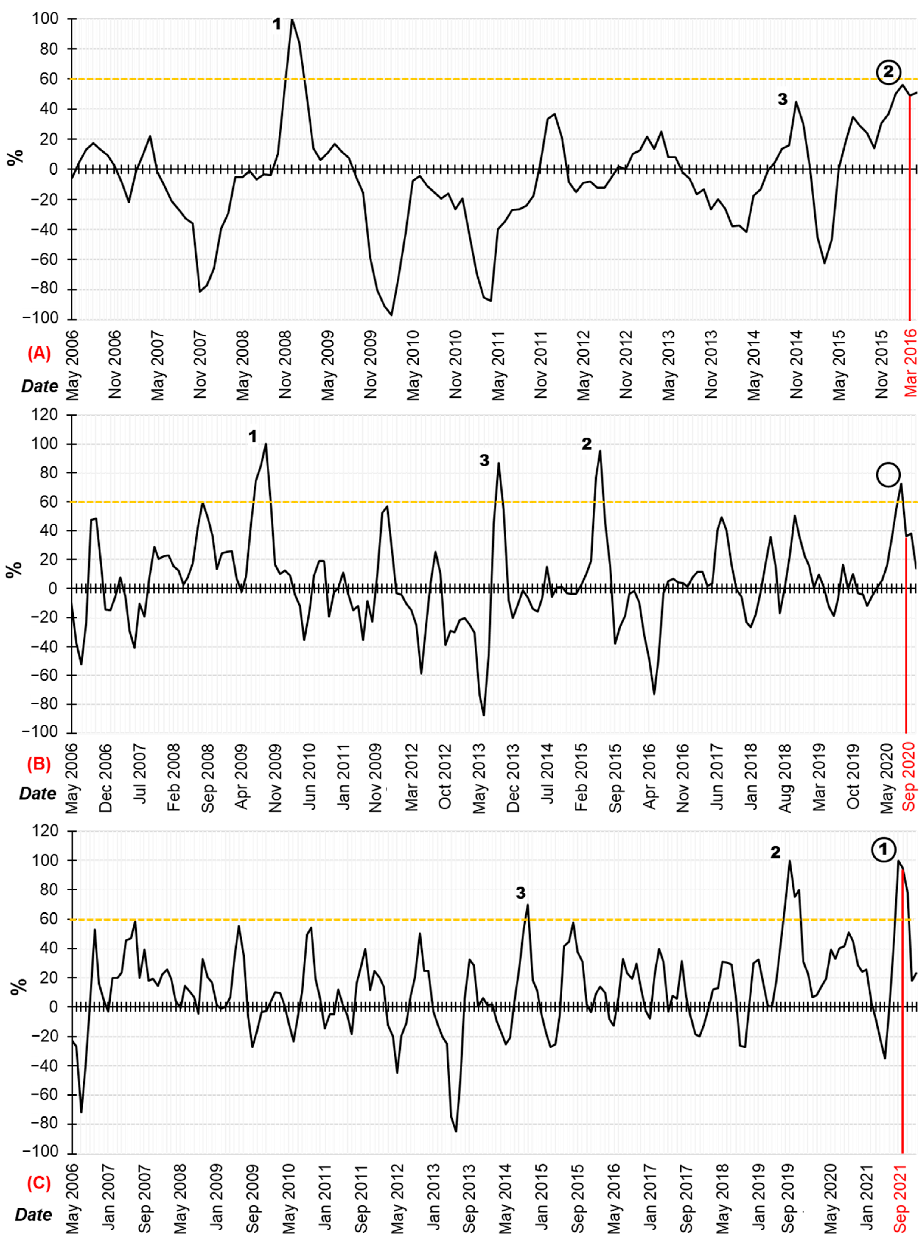
• ${\mathsf{\Delta }}_{\mathsf{\sigma }}$ > 1 or ${\mathsf{\Delta }}_{\mathsf{\sigma }}$ < −1 were used for sea surface height (SSH) and sea surface salinity (SSS) (both direct and inverse relationships of these parameters with the HAB risk are allowed [37,40]; the corresponding cells of Table 4 are marked with red).

Some cells in the Max/Min columns in Table 1 are also marked with red. This means that the current value of SST, PAR, WV, SSH, or SSS was an absolute extremum (or close to the absolute) on record (see Table 1). Herewith, for example, the entry “Max-2” indicates the fact of the registration of the second largest maximum in the entire history of observations. The yellow color in Table 4 indicates increased values of chlorophyll-a (CHL-A) concentration at ${\mathsf{\Delta }}_{\mathsf{\sigma }}$ > 1, which we considered an indicator of HAB occurrence.

The analysis of Table 4 shows that 1–4 months before the manifestations of all three studied intense HABs, increased values of SST and PAR were detected; herewith, two of the three studied HABs (near Hokkaido Island and the Kamchatka Peninsula) were accompanied by a high level of concentrations of CHL-a. Before all three HABs, a decrease in the components and/or in the resultant vectors of near-surface wind velocities was observed. Multidirectional SSH anomalies were registered before two HABs (near the island of Hokkaido and near the Kamchatka Peninsula). These results are confirmed, among other things, by previously conducted studies [9,23,76].

The SSS data have not demonstrated any clear HAB precursors; however, there are studies [77,78] indicating that in some cases, data on the salinity of the marine environment may be useful in the interest of studying the initiation and development of HAB phenomena. Possible reasons for the lack of salinity and HAB correlation in our experiments were probably related to the fact that the three studied HABs took place in ocean coastal water areas with relatively low salinity fluctuations. It is likely that salinity will be of greater importance in river and lake ecosystems, as well as in estuaries.

The spatial distributions of the investigated parameters were mapped and analyzed before the HABs, which demonstrated in greater detail the anomalies presented above in tabular form. Figure 4 shows examples of spatial distributions of deviations of absolute monthly mean values from the expected values (${\mathsf{\Delta }}_{abs}$) of the SST, PAR, and WV before the analyzed intense HABs.

The features of spatial distributions presented in Figure 4 agree with the data given in Table 4 and indicate that complex, spatially heterogeneous processes took place in the studied water areas before and during the intensive HABs. As is known, for example [6,17,19,79,80], attempts to analyze the sets of spatial distributions (similar to those shown in Figure 4) in detail help to make assumptions about the particularities of certain HABs’ formation mechanisms.

The results shown in Table 4 and in Figure 4, in general, indicate the prospects of using remote sensing methods and systems to register HAB precursors and indicators based on the study of long-term data on SST, PAR, VW, SSH, and CHL-A.

3.2. The HAB Risk

Figure 5a–c show graphs illustrating the dynamics of the HAB risk level obtained using the proposed function (exp. 6, 7). Red vertical lines in these figures mark the events of HABs, and yellow horizontal lines mark the levels of 60% of the historical maxima of HAB risk level, which were previously proposed to be considered as significant/threshold values.

Marks 1, 2, and 3 in Figure 5a–c show the extremes with the highest values of HAB risk level. The circles in Figure 5a–c indicate the extremes observed before the studied intense HABs. When the numbered extremum coincided with the extremum before the studied intense HABs, the number was placed in a circle (see Figure 5a,c). The circle without a number denotes the extremum before the studied HABs, which was not included in the number of three extrema with the highest values of HAB risk (see Figure 5b).

The analysis of Figure 5 shows the following:

• For all three studied areas, the local maxima of the HAB risk function (circles in Figure 5a–c) were observed ~1 month before the studied extreme HABs (red lines in Figure 5a–c).
• These maxima are above or at the level of 60% (yellow lines in Figure 5a–c) relative to the previously recorded absolute maxima of HAB risk level over the entire history of observations.

Of particular interest for discussion are the extremes that appeared above the levels of 60% in the graphs in Figure 5a–c, in addition to those that preceded the three major HABs under study. All such extremes are numbered in Figure 5a–c. Taking into account that for the three studied intensive HABs, the maxima of the risk function were observed beforehand (for ~1 month; see circles and red lines in Figure 5a–c, extremes with high levels of HAB risk (above 60%) can be considered precursors of such phenomena.

Further, it is worth checking whether these HAB precursor extremes correlate with real events. For this purpose, in this work, the search for and analysis of information confirming the presence of HABs in the three studied water areas, predicted using the numbered extremes indicated in Figure 5, were carried out. In most cases, except one (Avacha Bay near the Kamchatka Peninsula, June 2015), the fact of algal blooming was confirmed. These facts are demonstrated in detail in

Table 5. Generalized information about the HABs, the precursors of which were identified using the proposed approach.

Studied Water Area	HAB Risk Levels, % (3 Historical Maximums)	Time Interval for Registering the Extreme Value of HAB Risk Levels	HAB Registration Time Interval	Brief Description of the Registered HABs	References
Chiloe Island water area (Chile)	100.00	December 2008	January 2009	Harmful algae – A. Catenella Cell concentration—6,000,000 cells/L Consequences—intense reddish discoloration of water, intoxication of people, mass kill of salmon	[81,82]
	45.05	November 2014	December 2014	Harmful algae—T. Pseudonana Cell concentration—>500,000 cells/L Consequences—mass kill of salmon	[83,84]
	56.08	February 2016	March 2016	Harmful algae—P. cf. Verruculosa, A. Catenella Cell concentration—7000 cells/L (P. cf. Verruculosa), 250,000 cells/L (A. Catenella) Consequences—discoloration of water, mass kill of salmon	[76,85]
Avacha Bay water area (Russia)	100.00	September 2009	Intensive development of green algae throughout the year		[46,86]
	86.94	September 2013	October 2013	Harmful algae—Pseudo-nitzschia Cell concentration—>20,000 cells/L The consequences have not been recorded; however, at such cell concentration, in the countries of Europe and in the USA, toxicological control of marine products is to be carried out	[87,88]
	95.02	June 2015	Information about the HAB was not found		[89,90]
	72.49	August 2020	September 2020	Harmful algae—Karenia spp. Cell concentration—150,000 cells/L Consequences—water discoloration, foaming, mass death of hydrobionts	[8,23,79]
The island of Hokkaido water area (Japan)	69.89	October 2014	October 2014	Harmful algae—P. Dentatum Cell concentration—not established The consequences are a change in the color of the water to orange-yellow; the development of flowering did not pass into the harmful stage	[91,92]
	99.86	August 2019	August 2019	Harmful algae—C. polykrikoides, Ostreopsis sp., K. mikimotoi Cell concentration—10–70 cells/L (C. Polykrikoides), 10 cells/L (Ostreopsis sp., K. Mikimotoi) The consequences were not registered; the development of flowering did not become harmful	[93]
	100.00	August 2021	September 2021	Harmful algae—Kr. selliformis, Kr. mikimotoi Cell concentration—>10,000 cells/L (all types) The consequences were the mass kill of salmon and sea urchins. For this water area, a HAB of this scale is the first in history	[10]

, which provides generalized information about the HABs, the precursors of which were identified using the proposed approach.

The green color in Table 5 indicates three previously known events with intense HABs, which are mainly investigated in this paper. The remaining events were detected by identifying the maxima through the analysis of the HAB risk dynamics level obtained using the proposed function (see Figure 5a–c). Additionally, a search for public supporting information about the occurrence of HABs within the studied waters was carried out.

At the same time, it can be noted that the absence of evidence about HAB cases (for example, the case in Avacha Bay, June 2015) may be due to the lack of in situ observations in the studied waters during the relevant time periods.

Thus, as a result of the analysis, it was found that nine out of ten of the highest extremes of the proposed function for assessing the HAB risk level were accompanied by subsequent intensification of the blooming of various algae (including harmful ones, with dangerous concentrations of toxins in five cases).

Based on the conducted studies, it is shown that the proposed experimental function for assessing HAB risk level allowed adequately registering signals about three analyzed intensive HABs, as well as about six other confirmed phenomena of this type.

3.3. Long-Term Dynamics of Investigated Parameters in the Studied Water Areas

Table 6. Long-term trends (linear regression slope coefficients) of the significant environmental parameters SST, PAR, and VW for each month, registered for the water areas off Chiloe Island (Chile), Kamchatka Peninsula (Russia), and Hokkaido Island (Japan).

Sea Surface Temperature (SST), °C/Year
	Month	Jan	Feb	Mar	Apr	May	Jun	Jul	Aug	Sep	Oct	Nov	Dec
Area
Chiloe Island (Chile), 1981–2016		−0.0167	−0.0157	−0.0203	−0.007	−0.0028	0.0039	0.0073	0.0026	0.001	−0.0048	−0.0001	−0.0059
Kamchatka Peninsula (Russia), 1981–2020		0.0017	0.002	0.0009	0.0026	0.0193	0.0418	0.0537	0.0463	0.0196	0.0076	0.0076	0.0027
Hokkaido Island (Japan), 1981–2021		0.0074	−0.0032	−0.007	0.0039	0.0209	0.0332	0.0496	0.0407	0.0368	0.022	0.0227	0.0169
Photosynthetically active radiation (PAR) einstein/m2/day/year
	Month	Jan	Feb	Mar	Apr	May	Jun	Jul	Aug	Sep	Oct	Nov	Dec
Area
Chiloe Island (Chile), 2000–2016		0.5518	0.162	0.2624	−0.0186	−0.0565	0.0172	−0.0235	−0.1209	0.2002	0.2342	0.0332	−0.0111
Kamchatka Peninsula (Russia), 2000–2020		−0.0166	−0.0255	0.0154	0.0304	0.0039	0.0462	0.0093	−0.0354	−0.0749	0.0554	−0.0126	0.0006
Hokkaido Island (Japan), 2000–2021		0.014	−0.0649	−0.0925	0.0279	0.1031	−0.0008	0.1493	−0.0462	0.163	−0.027	−0.0164	−0.001
Wind velocity (WV), m/s/year
	Month	Jan	Feb	Mar	Apr	May	Jun	Jul	Aug	Sep	Oct	Nov	Dec
Area
Chiloe Island (Chile), 1979–2016		−0.0126	−0.0093	−0.0124	−0.0094	−0.0214	0.0164	0.0153	0.0029	−0.022	−0.0033	−0.01	0.0013
Kamchatka Peninsula (Russia), 1979–2020		0.0271	0.0377	0.0262	0.0143	0.0018	0.0144	0.0155	0.0241	0.0325	0.0287	0.0433	0.0398
Hokkaido Island (Japan), 1979–2021		0.0005	0.0188	0.003	0.0045	0.0087	0.0025	−0.0065	−0.0034	−0.0027	−0.0046	−0.0117	0.0212

shows the linear regression slope coefficients that characterize the long-term trends of the significant environmental parameters for the studied water areas for time periods from 16 to 42 years, depending on the time range of the parameter observation (see Table 1).

The values of the linear regression slope coefficients of the investigated parameters given in Table 6 were colored according to the color scale. Red indicates the highest rate of change of the parameter over time, and green indicates the lowest rate. This made it possible to preliminarily characterize the prospects for a decrease/increase in the HAB threat in the studied water areas. The blue frames in Table 6 indicate the seasons when intense HABs are to be expected (such seasons in different hemispheres of the Earth correspond to the coefficient $k_z$ = 2; see Table 3).

The analysis of the linear regression slope coefficients of the investigated parameters for each month in the studied water areas (Table 6) showed that these coefficients varied in a quite wide range. This fact reveals the complex, changing natural and climatic conditions of the studied coastal ecosystems. At the same time, it is necessary to note the following features that are essential for HAB forecasting:

• The strongest positive SST trends were recorded in the water areas adjacent to the Kamchatka Peninsula (Russia) and the island of Hokkaido (Japan) in the summer months (June−August). In the water area of Avacha Bay (Russia), the values of the linear regression slope coefficients in June, July, and August reached 0.042, 0.054, and 0.046 °C per year, respectively, which, in terms of the entire period of satellite observations (39 years for this area), is equivalent to warming by ~1.63 °C, 2.09 °C, and 1.81 °C, respectively. In the water area off the island of Hokkaido (Japan), the values of the linear regression slope coefficients in June, July, and August reached 0.032, 0.045, and 0.041 °C per year, respectively.
• The strongest negative trends for the WV parameter were manifested in the water area off the island of Chiloe (Chile) in the summer and autumn months (for the Southern Hemisphere, January−May). At this site, the linear regression slope coefficients in January, February, March, and April reached values of −0.013, −0.009, −0.012, and −0.009 m/s per year, which, in terms of the entire period of satellite observations (42 years for this water area), is equivalent to a decrease in wind velocity by ~−0.47 m/s, −0.34, −0.46, and −0.35 m/s, respectively.
• For the investigated PAR parameter, there is an increase in trends in the summer season (in January for the area off Chiloe Island (Chile), in June−July for the water areas of Avacha Bay near the Kamchatka Peninsula (Russia) and Hokkaido Island (Japan)). This may indicate the predominance of cloudless days in these summer months and the subsequent increase in the amount of incoming solar radiation. In the water area off Chiloe Island (Chile), the value of the PAR trend in January (summer in the Southern Hemisphere) reached 0.55 einstein/m²/day per year, which is equivalent to an increase in the amount of incoming radiation by 8.83 einstein/m²/day for the entire period of satellite observations (16 years for this water area). In the water area of Avacha Bay near the Kamchatka Peninsula (Russia), the values of the PAR trend in June reached 0.05 einstein/m²/day per year, which, in terms of the entire period of satellite observations (20 years for this water area), is equivalent to an increase in the amount of incoming radiation by ~1.0 einstein/m²/day. In the water area off Hokkaido (Japan), the values of the PAR trend in July reached 0.15 einstein/m²/day, which, in terms of the entire period of satellite observations (21 years), is equivalent to an increase in the amount of incoming radiation by ~3.15 einstein/m²/day.

Taking into account the above, in the studied waters of Avacha Bay near the Kamchatka Peninsula (Russia) and the island of Hokkaido (Japan), a clear positive dynamics of SST values was revealed as a key factor in the intensification of HABs. This may contribute to an increase in the frequency of the occurrence of such phenomena in the future. In the water area off the island of Chiloe (Chile), the factors whose trends indicate a high probability of aggravation of the HAB situation in the future are the increasing level of PAR and the decreasing WV.

4. Conclusions

Harmful algal blooms (HABs) occurring in various regions of the planet are a steadily increasing problem and require the attention of researchers. HABs harm the economy, worsen the well-being of people, and cause the death of marine organisms. Methods for monitoring and predicting these dangerous phenomena are of great importance.

The main purpose of this work was the analysis of long-term time series of archived satellite and model data on natural conditions in the waters where three intense HABs occurred, including off the island of Chiloe (Chile, 2016), adjacent to the Kamchatka Peninsula (Russia, 2020), and off the island of Hokkaido (Japan, 2021), to identify possible precursors and indicators of such specific natural phenomena.

The dynamics of a complex of significant environmental parameters in the studied water areas was investigated on the basis of the proposed approach to assessing HAB risks based on the statistical analysis of long-term satellite data series. For this purpose, satellite and model data were used on the sea surface temperature (NOAA OISST, since 1981); photosynthetically active radiation and chlorophyll-a concentration (MODIS Ocean Color SMI, since 2000); salinity and height of the sea surface (HYCOM, since 1993); and the characteristics of near-surface wind (NCEP CFSv2, since 1979). To overcome the limitations associated with the impact of hydrometeorological factors and hardware errors on the source data, the preparation and pre-processing of input information products and their aggregation were carried out to obtain representative monthly mean values of the studied significant environmental parameters.

In this effort, quantitative assessments of the dynamics of informative criteria about significant parameters of the marine environment and the surface layer of the atmosphere were used. The key informative criterion was the ratio of the absolute deviation of the studied parameter from the expected norm to the RMS dispersion of its values (${\mathsf{\Delta }}_{\mathsf{\sigma }}$). There were calculated and analyzed long-term time series of these criterion values according to heterogeneous satellite and model source data on significant environmental parameters for three test sites. The analysis and summary of the data obtained have shown that intense HABs were often preceded by excessive SST (up to ${\mathsf{\Delta }}_{\mathsf{\sigma }}$ ~1.99) and PAR (up to ${\mathsf{\Delta }}_{\mathsf{\sigma }}$ ~2.25) values, as well as low near-surface wind speed (up to ${\mathsf{\Delta }}_{\mathsf{\sigma }}$ ~−1.83). Providing for the obtained statistical data on the variability and peculiarities of significant environmental parameters before HAB intensifications, an approach and empirical function were proposed that allow us to assess the risk of such phenomena and reveal their precursors.

Retrospective analysis of satellite and model data using the proposed approach has allowed us to identify and analyze ten cases of high-risk HABs, nine of which were confirmed by field measurements, and one case was not accompanied by any reliable information about their existence. It should be noted that the lack of data on predicted HABs is not always a denial of their existence.

Based on the analysis of long-term trends in sea surface temperature, photosynthetically active radiation, and near-surface wind velocity, a danger of increased HAB frequency in the three studied water areas is predicted.

The proposed approach is promising for predicting intense HABs and can be used as a prospective strategy for investigating the conditions of occurrence of such specific phenomena. The proposed approach can be especially relevant in hard-to-reach areas of the World Ocean where in situ measurements are difficult.

Thus, the significance is revealed, and specific mechanisms are proposed for the integrated application of long-term time series of information products formed on the basis of satellite and model data to prevent the risks of anomalous HABs.

In the course of further research, the proposed approach to assessing HAB risk can be improved. The specific recommendations for the improvement of the proposed approach are optimizing preliminary empirical coefficients and developing a more advanced function for HAB risk occurrence. We believe it is expedient to develop such functions for particular HAB-exposed areas, taking into account specific natural and climatic conditions.

References

1. Anderson, D.M. Toxic Algal Blooms and Red Tides: A Global Perspective; Elsevier: Amsterdam, The Netherlands, 1989; pp. 11–16. [Google Scholar]
2. Konovalova, G.V. Red Tides in the Far Eastern Seas of Russia and Adjacent Aquatic Areas of the Pacific Ocean (A Review). Algologiya 1992, 2, 87–93. [Google Scholar]
3. Trainer, V.L.; Moore, S.K.; Hallegraeff, G.M.; Kudela, R.M.; Clément, A.; Mardones, J.I.; Cochlan, W.P. Pelagic harmful algal blooms and climate change: Lessons from nature’s experiments with extremes. Harmful Algae 2020, 91, 101591. [Google Scholar] [CrossRef] [PubMed]
4. Díaz, P.; Alvarez, G.; Varela, D.; Santos, I.E.; Diaz, M.; Molinet, C.; Seguel, M.; Aguilera, B.A.; Guzmán, L.; Uribe, E.; et al. Impacts of harmful algal blooms on the aquaculture industry: Chile as a case study. Perspect. Phycol. 2019, 6, 39–50. [Google Scholar] [CrossRef]
5. Bondur, V.G.; Zamshin, V.V.; Chvertkova, O.I. Space Study of a Red Tide-Related Environmental Disaster near Kamchatka Peninsula in September–October 2020. Dokl. Earth Sci. 2021, 497, 255–260. [Google Scholar] [CrossRef]
6. Orlova, T.Y.; Aleksanin, A.I.; Lepskaya, E.V.; Efimova, K.V.; Selina, M.S.; Morozova, T.V.; Stonik, I.V.; Kachur, V.A.; Karpenko, A.A.; Vinnikov, K.A.; et al. A massive bloom of Karenia species (Dinophyceae) off the Kamchatka coast, Russia, in the fall of 2020. Harmful Algae 2022, 120, 102337. [Google Scholar] [CrossRef] [PubMed]
7. Sakamoto, S.; Lim, W.A.; Lu, D.; Dai, X.; Orlova, T.; Iwataki, M. Harmful algal blooms and associated fisheries damage in East Asia: Current status and trends in China, Japan, Korea and Russia. Harmful Algae 2021, 102, 101787. [Google Scholar] [CrossRef] [PubMed]
8. Bondur, V.G.; Zamshin, V.V.; Chvertkova, O.I.; Matrosova, E.R.; Khodaeva, V.N. Analyzing Causes for the Environmental Disaster in Kamchatka in Autumn 2020 Due to a Red Tide Based on Satellite Data. Izv. Atmos. Ocean. Phys. 2021, 57, 937–949. [Google Scholar] [CrossRef]
9. Kuroda, H.; Taniuchi, Y.; Watanabe, T.; Azumaya, T.; Hasegawa, N. Distribution of Harmful Algae (Karenia spp.) in October 2021 Off Southeast Hokkaido, Japan. Front. Mar. Sci. 2022, 9, 841364. [Google Scholar] [CrossRef]
10. Bondur, V.G. Aerospace Methods and Technologies for Monitoring Oil and Gas Areas and Facilities. Izv. Atmos. Ocean. Phys. 2011, 47, 1007–1018. [Google Scholar] [CrossRef]
11. Keeler, R.N.; Bondur, V.G.; Vithanage, D. Sea truth measurements for remote sensing of littoral water. Sea Technol. 2004, 45, 53–58. [Google Scholar]
12. Bondur, V.G.; Filatov, N.N.; Grebenyuk, Y.V.; Dolotov, Y.S.; Zdorovennov, R.E.; Petrov, M.P.; Tsidilina, M.N. Studies of hydrophysical processes during monitoring of the anthropogenic impact on coastal basins using the example of Mamala Bay of Oahu Island in Hawaii. Oceanology 2007, 47, 769–787. [Google Scholar] [CrossRef]
13. Kartushinsky, A.V. Numerical Modeling Of The Hydrophysical Influence Effects on the Phytoplankton Distribution. Math. Biol. Bioinf. 2012, 7, 112–124. [Google Scholar] [CrossRef]
14. Bondur, V.G. Satellite monitoring and mathematical modelling of deep runoff turbulent jets in coastal water areas. In Waste Water—Evaluation and Management; InTechOpen: London, UK, 2011; pp. 155–180. ISBN 978-953-307-233-3. [Google Scholar] [CrossRef]
15. Zhao, J.; Ghedira, H. Monitoring red tide with satellite imagery and numerical models: A case study in the Arabian Gulf. Mar. Pollut. Bull. 2014, 79, 305–313. [Google Scholar] [CrossRef] [PubMed]
16. Bondur, V.G.; Zhurbas, V.M.; Grebenyuk, Y.V. Mathematical Modeling of Turbulent Jets of Deep-Water Sewage Discharge into Coastal Basins. Oceanology 2006, 46, 757–771. [Google Scholar] [CrossRef]
17. Bondur, V.G.; Vorobjev, V.E.; Grebenjuk, Y.V.; Sabinin, K.D.; Serebryany, A.N. Study of fields of currents and pollution of the coastal waters on the Gelendzhik Shelf of the Black Sea with space data. Izv. Atmos. Ocean. Phys. 2013, 49, 886–896. [Google Scholar] [CrossRef]
18. Binding, C.E.; Greenberg, T.A.; McCullough, G.; Watson, S.B.; Page, E. An analysis of satellite-derived chlorophyll and algal bloom indices on Lake Winnipeg. J. Great Lakes Res. 2018, 44, 436–446. [Google Scholar] [CrossRef]
19. Bondur, V.G.; Zamshin, V.V.; Chvertkova, O.I. Study of Anomalous Biogenic Pollution of the Marmara Sea Based on Satellite Data. Dokl. Earth Sc. 2022, 507, 968–976. [Google Scholar] [CrossRef]
20. Aleksanin, A.I.; Kim, V.; Orlova, T.Y.; Stonik, I.V.; Shevchenko, O.G. Phytoplankton of the Peter the Great Bay and Its Remote Sensing Problem. Oceanology 2012, 52, 219–230. [Google Scholar] [CrossRef]
21. Blondeau-Patissier, D.; Gower, J.F.R.; Dekker, A.G.; Phinn, S.R.; Brando, V.E. A review of ocean color remote sensing methods and statistical techniques for the detection, mapping and analysis of phytoplankton blooms in coastal and open oceans. Prog. Oceanogr. 2014, 123, 123–144. [Google Scholar] [CrossRef]
22. Aleksanin, A.I.; Orlova, T.Y.; Fomin, E.V.; Shevchenko, O.G. Prospects for Determining the Species Composition of Phytoplankton According to the MODIS Radiometer Data. Sovr. Probl. Distants. Zondir. Zemli Kosm. 2008, 2, 22–29. [Google Scholar]
23. Bondur, V.; Zamshin, V.; Chvertkova, O.; Matrosova, E.; Khodaeva, V. Detection and Analysis of the Causes of Intensive Harmful Algal Bloom in Kamchatka Based on Satellite Data. J. Mar. Sci. Eng. 2021, 9, 1092. [Google Scholar] [CrossRef]
24. Stumpf, R.P.; Tomlinson, M.C. Remote Sensing of Harmful Algal Blooms: Remote Sensing of Coastal Aquatic Environments; Springer: Dordrecht, The Netherlands, 2008; pp. 277–296. ISBN 978-1-4020-3099-4. [Google Scholar]
25. Kim, D.-W.; Jo, Y.-H.; Choi, J.-K.; Choi, J.-G.; Bi, H. Physical processes leading to the development of an anomalously large Cochlodinium polykrikoides bloom in the East sea/Japan sea. Harmful Algae 2016, 55, 250–258. [Google Scholar] [CrossRef] [PubMed]
26. Sukhanova, I.N.; Flint, M.V. Anomalous blooming of coccolithophorids over the eastern Bering Sea shelf. Oceanology 1998, 38, 502–505. [Google Scholar]
27. Orlova, T.Y. Red tides and toxic microalgae in the Far Eastern seas of Russia. Vestn. DVO RAN 2005, 1, 27–31. [Google Scholar]
28. Vershinin, A.O.; Orlova, T.Y. Toxic and harmful algae in the coastal waters of Russia. Oceanology 2008, 48, 524–537. [Google Scholar] [CrossRef]
29. Shoman, N.Y. The Combined Effect of Light, Temperature and Nitrogen Availability on the Growth Rate and Chlorophyll a Content in Marine Diatoms. Available online: https://www.dissercat.com/content/sovmestnoe-deistvie-sveta-temperatury-i-obespechennosti-azotom-na-skorost-rosta-i-soderzhani (accessed on 20 May 2023).
30. Beardall, J.; Raven, J.A. The potential effects of global climate change on microalgal photosynthesis, growth and ecology. Phycologia 2004, 43, 26–40. [Google Scholar] [CrossRef]
31. León-Muñoz, J.; Urbina, M.A.; Garreaud, R.; Iriarte, J.L. Hydroclimatic conditions trigger record harmful algal bloom in western Patagonia (summer 2016). Sci. Rep. 2018, 8, 1330. [Google Scholar] [CrossRef]
32. Paerl, H.W.; Huisman, J. Climate change: A catalyst for global expansion of harmful cyanobacterial blooms. Environ. Microbiol. Rep. 2009, 1, 27–37. [Google Scholar] [CrossRef]
33. Moradi, M.; Kabiri, K. Red tide detection in the Strait of Hormuz (east of the Persian Gulf) using MODIS fluorescence data. Int. J. Remote Sens. 2012, 33, 1015–1028. [Google Scholar] [CrossRef]
34. Wei, G.; Tang, D.; Wang, S. Distribution of chlorophyll and harmful algal blooms (HABs): A review on space based studies in the coastal environments of Chinese marginal seas. Adv. Space Res. 2008, 41, 12–19. [Google Scholar] [CrossRef]
35. Ahn, Y.H.; Shanmugam, P. Detecting the red tide algal blooms from satellite ocean color observations in optically complex Northeast-Asia Coastal waters. Remote Sens. Environ. 2006, 103, 419–437. [Google Scholar] [CrossRef]
36. Hu, C.; Feng, L. Modified MODIS fluorescence line height data product to improve image interpretation for red tide monitoring in the eastern Gulf of Mexico. J. Appl. Remote Sens. 2016, 11, 012003. [Google Scholar] [CrossRef]
37. Tang, D.L.; Kawamura, H.; Doan-Nhu, H.; Takahashi, W. Remote sensing oceanography of a harmful algal bloom off the coast of southeastern Vietnam. J. Geophys. Res. Ocean. 2004, 109, C03014. [Google Scholar] [CrossRef]
38. Pugach, S.P.; Pipko, I.I.; Shakhova, N.E.; Shirshin, E.A.; Perminova, I.V.; Gustafsson, O.; Bondur, V.G.; Ruban, A.S.; Semiletov, I.P. Dissolved organic matter and its optical characteristics in the Laptev and East Siberian seas: Spatial distribution and interannual variability (2003–2011). Ocean. Sci. 2018, 14, 87–103. [Google Scholar] [CrossRef]
39. Xiao, X.; Agustí, S.; Pan, Y.; Yu, Y.; Li, K.; Wu, J.; Duarte, C.M. Warming Amplifies the Frequency of Harmful Algal Blooms with Eutrophication in Chinese Coastal Waters. Environ. Sci. Technol. 2019, 53, 13031–13041. [Google Scholar] [CrossRef] [PubMed]
40. Laabir, M.; Jauzein, C.; Genovesi, B.; Masseret, E.; Grzebyk, D.; Cecchi, P.; Vaquer, A.; Perrin, Y.; Collos, Y. Influence of temperature, salinity and irradiance on the growth and cell yield of the harmful red tide dinoflagellate Alexandrium catenella colonizing Mediterranean waters. J. Plankton Res. 2011, 33, 1550–1563. [Google Scholar] [CrossRef]
41. Kopelevich, O.V.; Vazyulya, S.V.; Grigoriev, A.V.; Khrapko, A.N.; Sheberstov, S.V.; Sahling, I.V. Penetration of visible solar radiation in waters of the Barents Sea depending on cloudiness and coccolithophore blooms. Oceanology 2017, 57, 445–453. [Google Scholar] [CrossRef]
42. Ranjbar, M.H.; Hamilton, D.P.; Etemad-Shahidi, A.; Helfer, F. Impacts of atmospheric stilling and climate warming on cyanobacterial blooms: An individual-based modelling approach. Water Res. 2022, 221, 118814. [Google Scholar] [CrossRef]
43. Bondur, V.G.; Grebenyuk, Y.V.; Sabinin, K.D. Variability of internal tides in the coastal water area of Oahu Island (Hawaii). Oceanology 2008, 48, 611–621. [Google Scholar] [CrossRef]
44. Bondur, V.G.; Grebenyuk, Y.V.; Sabynin, K.D. The spectral characteristics and kinematics of short-period internal waves on the Hawaiian shelf. Izv. Atmos. Ocean. Phys. 2009, 45, 598–607. [Google Scholar] [CrossRef]
45. Wilson, C.; Adamec, D. Correlations between surface chlorophyll and sea surface height in the tropical Pacific during the 1997–1999 El Niño-Southern Oscillation event. J. Geophys. Res. Ocean. 2001, 106, 31175–31188. [Google Scholar] [CrossRef]
46. Ocheretyana, S.O.; Klochkova, N.G.; Klochkova, T.A. Seasonal species composition of “green tide”-forming algae from Avacha Bay and effect of anthropogenic pollution on physiology and growth of some green algae. Vestn. KamchatGTU 2015, 33, 30–36. [Google Scholar] [CrossRef]
47. Anderson, D.M.; Glibert, P.M.; Burkholder, J.M. Harmful algal blooms and eutrophication: Nutrient sources, composition, and consequences. Estuaries 2002, 25, 704–726. [Google Scholar] [CrossRef]
48. Bakhtiar, M.; Rezaee Mazyak, A.; Khosravi, M. Ocean Circulation to Blame for Red Tide Outbreak in the Persian Gulf and the Sea of Oman. Int. J. Marit. Technol. 2020, 13, 31–39. [Google Scholar]
49. Heisler, J.; Glibert, P.M.; Burkholder, J.M.; Anderson, D.M.; Cochlan, W.; Dennison, W.C.; Dortch, Q.; Gobler, C.J.; Heil, C.A.; Humphries, E.; et al. Eutrophication and harmful algal blooms: A scientific consensus. Harmful Algae 2008, 8, 3–13. [Google Scholar] [CrossRef]
50. Konovalova, G.V. Krasnyye Prilivy u Vostochnoy Kamchatki (Atlas-Spravochnik) [Red Tides Near Eastern Kamchatka (Atlas-Reference Book)]; Kamshat: Petropavlovsk-Kamchatsky, Russia, 1995; 57p. [Google Scholar]
51. Jacques-Coper, M.; Segura, C.; de la Torre, M.B.; Valdebenito Muñoz, P.; Vásquez, S.I.; Narváez, D.A. Synoptic-to-intraseasonal atmospheric modulation of phytoplankton biomass in the inner sea of Chiloé, Northwest Patagonia (42.5°–43.5°S, 72.5°–74°W), Chile. Front. Mar. Sci. 2023, 10, 1160230. [Google Scholar] [CrossRef]
52. Narváez, D.A.; Vargas, C.A.; Cuevas, L.A.; García-Loyola, S.A.; Lara, C.; Segura, C.; Tapia, F.J.; Broitman, B.R. Dominant scales of subtidal variability in coastal hydrography of the Northern Chilean Patagonia. J. Mar. Syst. 2019, 193, 59–73. [Google Scholar] [CrossRef]
53. Lomtev, V.L. To The Structure And History Of Kamchatka Canyon (Eastern Kamchatka). Geol. Miner. Resour. World Ocean 2018, 3, 37–61. [Google Scholar] [CrossRef]
54. Luchin, V.A.; Kruts, A.A. Properties of cores of the water masses in the Okhotsk Sea. Izv. TINRO 2016, 184, 204–218. [Google Scholar] [CrossRef]
55. Mekler, G.K. Hokkaido, 2nd ed.; Popov, K.M., Kovyzhenko, V.V., Eds.; USSR Academy of Sciences, Institute of Oriental Studies: Moscow, Russia, 1986; p. 163. [Google Scholar]
56. Reynolds, R.W.; Banzon, V.F.; NOAA CDR Program. NOAA Optimum Interpolation 1/4 Degree Daily Sea Surface Temperature (OISST) Analysis, 2nd ed.; National Centers for Environmental Information: Asheville, NC, USA, 2008. [Google Scholar]
57. NASA Goddard Space Flight Center; Ocean Ecology Laboratory; Ocean Biology Processing Group. Moderate-resolution Imaging Spectroradiometer (MODIS) Aqua Level-3 Mapped Photosynthetically Available Radiation, Version 2022 Data; NASA OB.DAAC: Greenbelt, MD, USA. [CrossRef]
58. NASA Goddard Space Flight Center; Ocean Ecology Laboratory; Ocean Biology Processing Group. Moderate-resolution Imaging Spectroradiometer (MODIS) Terra Level-3 Binned Photosynthetically Available Radiation, Version 2022 Data; NASA OB.DAAC: Greenbelt, MD, USA. [CrossRef]
59. NASA Goddard Space Flight Center; Ocean Ecology Laboratory; Ocean Biology Processing Group. Moderate-resolution Imaging Spectroradiometer (MODIS) Aqua Level-3 Binned Chlorophyll, Version 2022 Data; NASA OB.DAAC: Greenbelt, MD, USA. [CrossRef]
60. NASA Goddard Space Flight Center; Ocean Ecology Laboratory; Ocean Biology Processing Group. Moderate-resolution Imaging Spectroradiometer (MODIS) Terra Level-3 Binned Chlorophyll, Version 2022 Data; NASA OB.DAAC: Greenbelt, MD, USA. [CrossRef]
61. Chassignet, E.; Hurlburt, H.; Metzger, E.; Smedstad, O.; Cummings, J.; Halliwell, G.; Bleck, R.; Baraille, R.; Wallcraft, A.; Lozano, C.; et al. Global Ocean Prediction with the Hybrid Coordinate Ocean Model (HYCOM). Oceanography 2009, 22, 64–75. [Google Scholar] [CrossRef]
62. Saha, S.; Moorthi, S.; Wu, X.; Wang, J.; Nadiga, S.; Tripp, P.; Behringer, D.; Hou, Y.-T.; Chuang, H.; Iredell, M.; et al. NCEP Climate Forecast System Version 2 (CFSv2) 6-Hourly Products. Available online: https://rda.ucar.edu/datasets/ds094.0/ (accessed on 28 June 2023).
63. Hobday, A.J.; Oliver, E.C.J.; Sen Gupta, A.; Benthuysen, J.A.; Burrows, M.T.; Donat, M.G.; Holbrook, N.J.; Moore, P.J.; Thomsen, M.S.; Wernberg, T.; et al. Categorizing and naming marine heatwaves. Oceanography 2018, 31, 162–173. [Google Scholar] [CrossRef]
64. Jiang, L.; Zhao, X.; Wang, L. Long-Range Correlations of Global Sea Surface Temperature. PLoS ONE 2016, 11, e0153774. [Google Scholar] [CrossRef] [PubMed]
65. Hobday, A.J.; Alexander, L.V.; Perkins, S.E.; Smale, D.A.; Straub, S.C.; Oliver, E.C.J.; Benthuysen, J.A.; Burrows, M.T.; Donat, M.G.; Feng, M.; et al. A hierarchical approach to defining marine heatwaves. Prog. Oceanogr. 2016, 141, 227–238. [Google Scholar] [CrossRef]
66. McGillicuddy, D.J. Models of harmful algal blooms: Conceptual, empirical, and numerical approach. J. Mar. Syst. 2010, 83, 105–107. [Google Scholar] [CrossRef] [PubMed]
67. Anderson, C.R.; Siegel, D.A.; Kudela, R.M.; Brzezinski, M.A. Empirical models of toxigenic Pseudo-nitzschia blooms: Potential use as a remote detection tool in the Santa Barbara Channel. Harmful Algae 2009, 8, 478–492. [Google Scholar] [CrossRef]
68. Hamilton, G.; McVinish, R.; Mengersen, K. Bayesian model averaging for harmful algal bloom prediction. Ecol. Appl. A Publ. Ecol. Soc. Am. 2009, 19, 1805–1814. [Google Scholar] [CrossRef] [PubMed]
69. Hongwon, Y. Prediction model of algal blooms using logistic regression and confusion matrix. Int. J. Electr. Comput. Eng. 2021, 11, 2407. [Google Scholar] [CrossRef]
70. Izadi, M.; Sultan, M.; Kadiri, R.E.; Ghannadi, A.; Abdelmohsen, K.A. Remote Sensing and Machine Learning-Based Approach to Forecast the Onset of Harmful Algal Bloom. Remote Sens. 2021, 13, 3863. [Google Scholar] [CrossRef]
71. Raine, R.; McDermott, G.; Silke, J.; Lyons, K.; Nolan, G.; Cusack, C. A simple short range model for the prediction of harmful algal events in the bays of southwestern Ireland. J. Mar. Syst. 2010, 83, 150–157. [Google Scholar] [CrossRef]
72. Rousso, B.Z.; Bertone, E.; Stewart, R.; Hamilton, D.P. A systematic literature review of forecasting and predictive models for cyanobacteria blooms in freshwater lakes. Water Res. 2020, 182, 115959. [Google Scholar] [CrossRef]
73. Vasilenko, N.V.; Medvedeva, A.V.; Aleskerova, A.A.; Kubryakov, A.A.; Stanichny, S.V. Features of cyanobacteria blooms in the central part of the Sea of Azov from satellite data. Sovr. Probl. DZZ Kosm. 2021, 18, 166–180. [Google Scholar] [CrossRef]
74. Gavrilenko, G.G.; Zdorovennova, G.E.; Zdorovennov, R.E.; Palshin, N.I.; Efremova, T.V.; Terzhevik, A.Y. Spatio-temporal variability of photosynthetically active solar radiation flow in a shallow lake during the open water period. Obshchest. Sreda Razvit. 2015, 3, 186–192. [Google Scholar]
75. Horn, H.; Paul, L. Interactions between Light Situation, Depth of Mixing and Phytoplankton Growth during the Spring Period of Full Circulation. Int. Rev. Der Gesamten Hydrobiol. Und Hydrogr. 1984, 69, 507–519. [Google Scholar] [CrossRef]
76. Clement, A.; Lincoqueo, L.; Saldivia, M.; Brito, C.G.; Muñoz, F.; Fernández, C.; Pérez, F.; Maluje, C.P.; Correa, N.; Moncada, V.; et al. Exceptional summer conditions and HABs of Pseudochattonella in Southern Chile create record impacts on salmon farms. Harmful Algae News 2016, 53, 1–23. [Google Scholar]
77. Band-Schmidt, C.J.; Morquecho, L.; Lechuga-Devéze, C.H.; Anderson, D.M. Effects of growth medium, temperature, salinity and seawater source on the growth of Gymnodinium catenatum (Dinophyceae) from Bahía Concepción, Gulf of California, Mexico. J. Plankton Res. 2004, 26, 1459–1470. [Google Scholar] [CrossRef]
78. Xu, N.; Duan, S.; Li, A.; Zhang, C.; Cai, Z.; Hu, Z. Effects of temperature, salinity and irradiance on the growth of the harmful dinoflagellate Prorocentrum donghaiense Lu. Harmful Algae 2010, 9, 13–17. [Google Scholar] [CrossRef]
79. Alexanin, A.; Kachur, V.; Khramtsova, A.; Orlova, T. Methodology and Results of Satellite Monitoring of Karenia Microalgae Blooms, That Caused the Ecological Disaster off Kamchatka Peninsula. Remote Sens. 2023, 15, 1197. [Google Scholar] [CrossRef]
80. Xing, Q.; Hu, C.; Tang, D.; Tian, L.; Tang, S.; Wang, X.; Lou, M.; Gao, X. World’s Largest Macroalgal Blooms Altered Phytoplankton Biomass in Summer in the Yellow Sea: Satellite Observations. Remote Sens. 2015, 7, 12297–12313. [Google Scholar] [CrossRef]
81. Mardones, J.; Clement, A.; Rojas, X.; Aparicio, C. Alexandrium catenella during 2009 in Chilean waters, and recent expansion to coastal ocean. Harmful Algae News 2010, 41, 8–9. [Google Scholar]
82. Harmful Algal Event Database. Available online: http://haedat.iode.org/viewEvent.php?eventID=5752/ (accessed on 18 June 2023).
83. Mardones, J. Screening of Chilean fish-killing microalgae using a gill cell-based assay. Lat. Am. J. Aquat. Res. 2020, 48, 329–335. [Google Scholar] [CrossRef]
84. Harmful Algal Event Database. Available online: http://haedat.iode.org/viewEvent.php?eventID=5976 (accessed on 18 June 2023).
85. Harmful Algal Event Database. Available online: http://haedat.iode.org/viewEvent.php?eventID=5740 (accessed on 18 June 2023).
86. Ocheretyana, S.O.; Klochkova, N.G. Late Autumn Composition Of Green Ephemeral Algae In The Bunkering Areas Of The Fleet In Avacha Bay (Southeastern Kamchatka). Vestn. KamchatGTU 2010, 11, 58–64. [Google Scholar]
87. Lepskaya, E.V.; Tepnin, O.B.; Kolomeitsev, V.V.; Ustimenko, N.V.; Sergeenko, N.V.; Vinogradova, D.S.; Sviridenko, V.D.; Pokhodina, M.A.; Schegolkova, V.A.; Maksimenkov, V.V.; et al. Historical Review Of Studies Of Avachinskaya Bay And Principle Results Of Complex Ecological Monitoring 2013. Res. Aquat. Biol. Resour. Kamchatka North-West Part Pac. Ocean. 2014, 34, 5–21. [Google Scholar]
88. Anderson, P. Design and Implementation of Some Harmful Algal Monitoring Systems; IOC Technical Series; Intergovernmental Oceanographic Commission: Paris, France, 1996; 102p. [Google Scholar]
89. Weitkamp, L. Recent ocean conditions and trends of Pacific salmon from Alaska to California. Probl. Fish. 2021, 22, 27–34. [Google Scholar] [CrossRef]
90. McCabe, R.M.; Hickey, B.M.; Kudela, R.M.; Lefebvre, K.A.; Adams, N.G.; Bill, B.D.; Gulland, F.M.D.; Thomson, R.E.; Cochlan, W.P.; Trainer, V.L. An unprecedented coastwide toxic algal bloom linked to anomalous ocean conditions. Geophys. Res. Lett. 2016, 43, 10366–10376. [Google Scholar] [CrossRef] [PubMed]
91. Shimada, H.; Sakamoto, S.; Yamaguchi, M.; Imai, I. First record of two warm-water HAB species Chattonella marina (Raphidophyceae) and Cochlodinium polykrikoides (Dinophyceae) on the west coast of Hokkaido, northern Japan in summer 2014. Reg. Stud. Mar. Sci. 2016, 7, 111–117. [Google Scholar] [CrossRef]
92. Inaba, N.; Kodama, I.; Nagai, S.; Mori, K.; Imai, I. Distribution of Growth-Limiting Bacteria Against Harmful Algal Bloom Species at Shinori Fishing Port and Surrounding Environments. Civil Engineering Research Institute for Cold Region (CERI) 2023, 841, 2–10. [Google Scholar]
93. Shimada, H. Long-term fluctuation of red tide and shellfish toxin along the coast of Hokkaido (Review). Sci. Rep. Hokkaido Fish. Res. Inst. 2021, 100, 1–12. [Google Scholar]
Figure 1. A generalized flowchart of the main factors, indicators, and negative consequences of HABs.
Remotesensing 15 05308 g001
Figure 2. The studied water areas. (A) Near the island of Chiloe (Chile), (B) Avacha Bay adjacent to the Kamchatka Peninsula (Russia), (C) near the island of Hokkaido (Japan). (D) Examples of the consequences of HABs in these areas.
Remotesensing 15 05308 g002
Figure 3. Generalized flowchart of the study.
Remotesensing 15 05308 g003
Figure 4. Spatial distributions of deviations of absolute monthly mean values of significant environmental parameters (1) in the water area off Chiloe Island for (a1) SST for January 2016, (b1) PAR for March 2016, (c1) WV for January 2016; (2) in the water area of Avacha Bay for (a2) SST for July 2020, (b2) PAR for July 2020, (c2) WV for August 2020; (3) in the water area off Hokkaido Island for (a3) SST for July 2021, (b3) PAR for July 2021, (c3) WV for September 2021.
Remotesensing 15 05308 g004
Figure 5. The dynamics of HAB risk level calculated according to the proposed methodology (A) in the water area of Chiloe Island (2006–2016); (B) in the water area off Avacha Bay (2006–2020); (C) in the area off Hokkaido Island (2006–2021).
Remotesensing 15 05308 g005