Abstract
The article presents the results of transient electromagnetic (TEM) prospecting surveys using an unmanned aerial system carried out at Lake Baikal, which is a unique geoelectrical setting where low-resistivity lacustrine sediments are located under a relatively isotropic water body. The task was to investigate the possibility of using a drone-based TEM survey to delineate the electrical stratigraphy of the subsurface at depths between 50 and 300 m, separated into layers and blocks. A new version of the SibGIS UAV-TEM unmanned system was used, significantly improved compared to the prototype previously described in the literature. The current switch providing bipolar current pulses connected to a grounded electrical line was the source of the electromagnetic field in the geological environment. The hexacopter carrying a measuring system consisting of 18-bit ADC and sensor—analog of 50 × 50 loop, was the receiving system. We measured survey data of 16 traverses over the Baikal going from the shore to the depths. Significant attention is being paid to a new approach to data inversion. For fast interpretation of the TEM data, we used the Sτ-method, which allows for tracing the change in the apparent longitudinal conductivity with depth. It is shown that thanks to the new sensor and current switch, the data quality has increased significantly; now, the UAV system can register sounding curves up to 1 ms. As a result, new data on the geological structure of the shelf zone of Lake Baikal were obtained. They had a good fundamental agreement with the predecessor data obtained from terrestrial measurements (from ice cover), allowing us to conclude that the UAV-TEM technology can already replace conventional ground-based electromagnetic surveys.
1. Introduction
In the first two decades of the 21st century, airborne electromagnetic surveying has become widespread. Presently, we are witnessing the development of a new branch of electromagnetic exploration: electromagnetic prospecting surveys use drones. The receiver, sensor, and computer can be hung beneath an unmanned aircraft that flies on autopilot at low altitudes with terrain flow. For collecting geophysical data, UAV technology has several advantages over conventional airborne platforms, including low safe flight altitude, ensuring a high resolution, and low flight speed, ensuring accuracy. However, modern drones have limited endurance and carrying capacity [1]. Nevertheless, in comparison to ground surveying, a drone can collect hundreds of thousands of readings in several days [2].
There are two types of control source electromagnetic surveys carried out using drones: frequency domain methods and transient (time-domain) methods (TEM). The frequency domain EM has been used more, and technology and software for pre-processing and interpretation have developed much better [3,4,5]. Time domain UAV-airborne technologies is a new page of the EM survey, and only a few works are known from the literature so far [6], with the exception of articles by the authors [2,7,8].
However, we consider TEM more promising for the search for hidden mineral deposits at the depth range of between 100 and 500 m [8]. The first version of our instrument [2,8] has been used for geoelectric prospecting since 2020. Unfortunately, this instrument had a number of significant limitations: rather heavy sensors were used, which reduced the flight endurance time; the current switch could not provide the necessary pulse frequency to record—only two readings per second. This did not allow for achieving a stable recording of late field decay times. In addition, for the interpretation of airborne data, we used software originally developed for ground-based TEM data, not effective for interpreting thousands of readings per day. That is why it was not possible to do preprocessing and interpretation of UAV-collected TEM data for a reasonable time. Therefore, the results of the summer survey of 2020, which took one day to collect, were processed and published only in February 2021 [2], which is, of course, unacceptable for commercial technology. In this article, we want to show the progress in the development of our SibGIS UAV-TEM technology, both in relation to the data processing system and in relation to the measuring and generating parts, and to prove that the modern version of the UAV-TEM technique is already a fairly serious geophysical tool.
2. Materials and Methods
2.1. Instrumentation
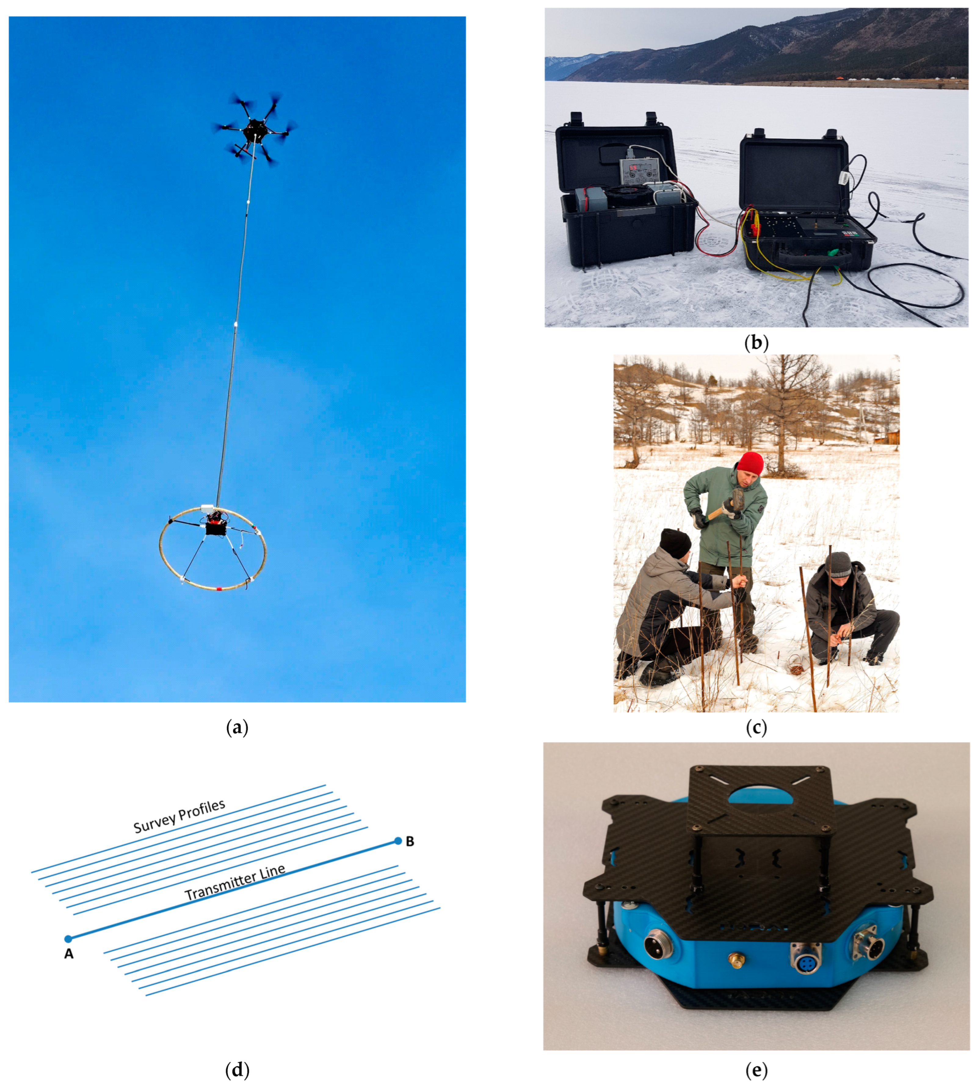
The electrical prospecting system consisted of ground and airborne parts; the receiver was on the aircraft, and the transmitter was on the ground (Figure 1).

Figure 1.
(a) UAV with receiving system, (b) EGI-5000 current source, (c) standard groundings, (d) standard geometry of survey, and (e) 18-bit 100 kHz ADC.
The electromagnetic field in the geological environment creates the transmitter, consisting of the galvanically grounded electric line several kilometers long, with a current source attached to it. The transmitter CTU-HV was used to supply square-pulsed current to the electrical line (Figure 1a). Grounding at the ends of the line were 25 steel electrodes 1 m long (Figure 1c), connected to each other and to the supply line using a copper cable. The transmitter produced bipolar 50% duty cycle current pulses. The duration of the current pulses was 10 ms on and 10 ms off. The CTU-HV consists of two separate units: one is a current-stabilized source, and the other is a square wave pulse generator (Figure 1b).
The specifications of the transmitter CTU-HV are presented in Table 1. The transmitter was packed in a protected housing. Synchronization with the receiver occurs using GNSS time.

Table 1.
Specification of the transmitter CTU-HV.
The measuring system, which was located on the aircraft, consisted of a receiving inductive sensor—an analog of a 50 × 50 m loop (Figure 1a), an analog-to-digital converter “MARS” (Figure 1e), and a minicomputer recorder. The specifications of the ADC are presented in Table 2.
Table 2.
Specification of the ADC and registrar.
The receiving sensor used is a multi-turn loop with a 0.9-m diameter. It is a special adaptation for the SibGIS UAV-TEM system of the PDI-50 sensor known on the Russian market in the 1980s [developed by A.K. Zakharkin (SNIIGIMS, Novosibirsk, Russia)] [9]. The effective area Q (Q = Sn, where S is the surface area of the loop and n is the number of turns) is 2500 m2. The specifications of the sensor are presented in Table 3. The loop was equipped with a self-induction compensator. The loop weighed slightly more than 3 kg (in the first versions of the system, the weight exceeded 7 kg). An important, and even often decisive, role in obtaining high-quality survey results is the sensor suspension system, which must ensure its horizontal position at any speed of the UAV and prevent it from rotating and swaying during the flight mission. The sensor was located at a distance of 8 m under the UAV.
Table 3.
Specification of the receiving loop.
The unmanned carrier (Figure 1a) was a standard SibGIS UAS hexacopter with a 1.2-m frame and payload of up to 10 kg. Its feature is a reduced level of electromagnetic interference [10].
2.2. Technique of Measurement
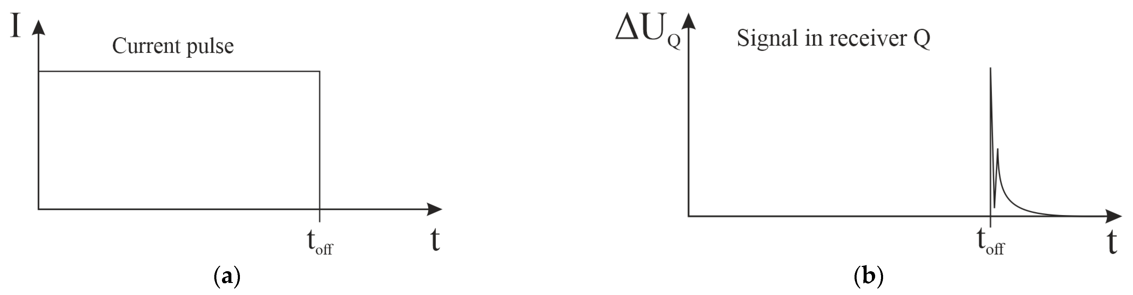
Usually, when performing a geophysical survey using the SibGIS UAS system, the flight is carried out with a terrain drape, for which a special flight planner is used [10]. However, in this case, the flight was carried out over Lake Baikal at a constant height of 15 m above the water (ice). The transmitter was a 2200-m-long grounded AB line. Iron poles were lowered into the ice holes and used as groundings. The unmanned aircraft system flew along profiles over the survey area, continuously resisting TEM signals at a frequency of 100 kHz. In the recording of the transient pulse, the maximum delay was 10 ms. Figure 2 demonstrates the shape of the current pulse in the transmitter line AB (a) and the signal in the receiver loop Q (b).
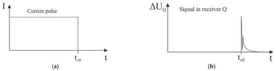
Figure 2.
The shape of the current pulse in the transmitter line AB (a) and the signal in the receiver loop Q (b).
TEM data for each flight were saved in a separate file. Since a single flight may consist of data from multiple profiles, the data collected from each profile were subsequently stored in a separate file that was necessary for the convenience of further data processing.
The processing procedure was as follows [2]:
- -
- after the current was turned off, recorded transient EM signals were extracted from the continuous data set;
- -
- suppression of industrial noise;
- -
- elimination of the trend;
- -
- robust smoothing in a 2D sliding window;
- -
- interpolation of TEM readings on the logarithmic time scale;
- -
- each measurement point was merged with its corresponding x, y, and z coordinates by the software.
3. Results
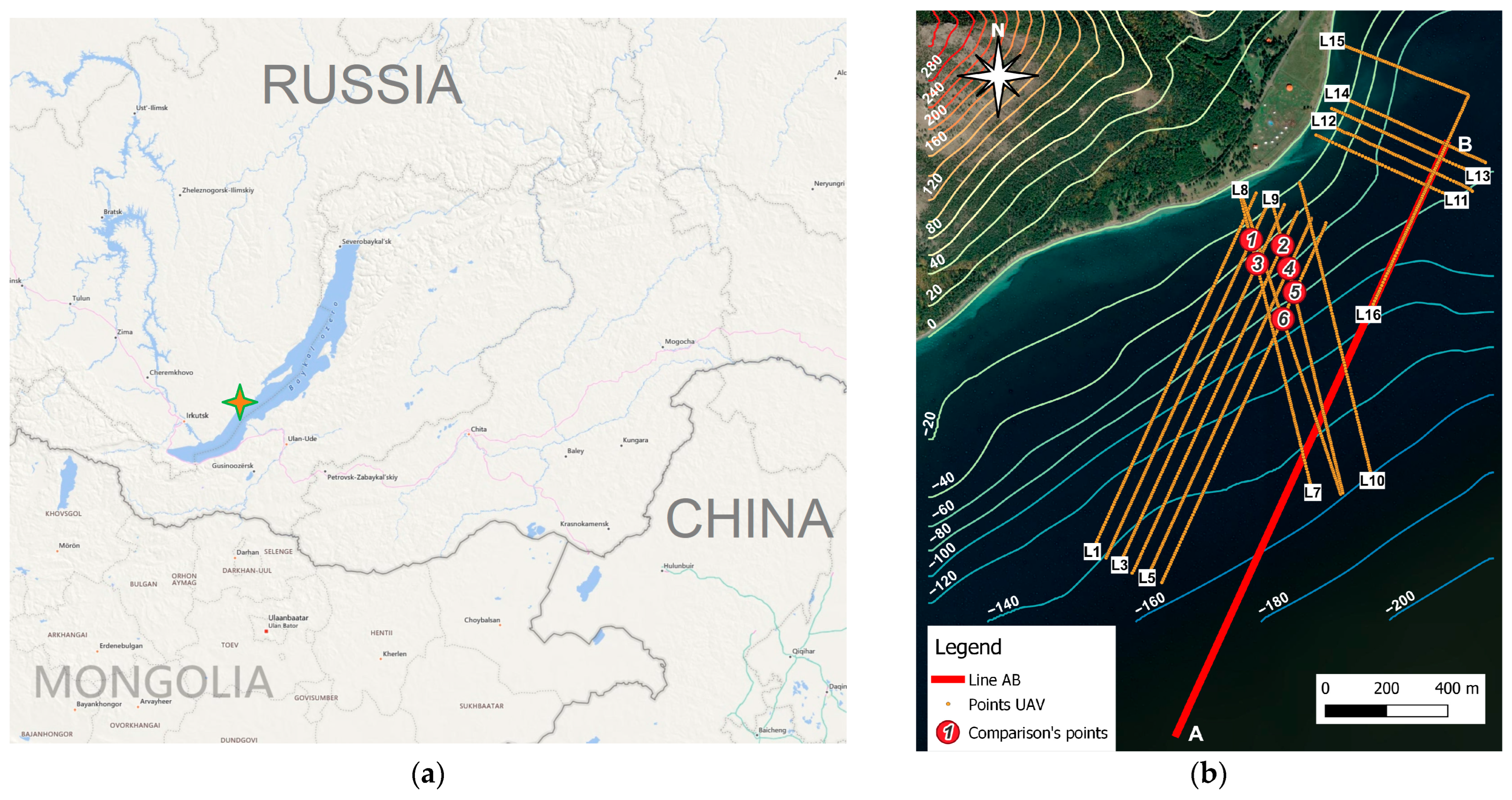
Figure 3 depicts the location of profiles on the Bolshoe Goloustnoe site. A total of 16 profiles were performed: six of them are parallel to line AB, four are inclined, and six are perpendicular to the line.
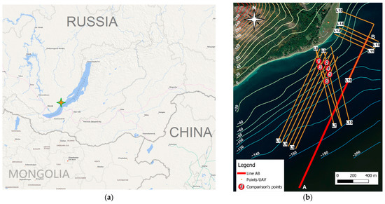
Figure 3.
Location of the site Bolshoe Goloustnoye at Lake Baikal (a) and survey profiles on the site (b).
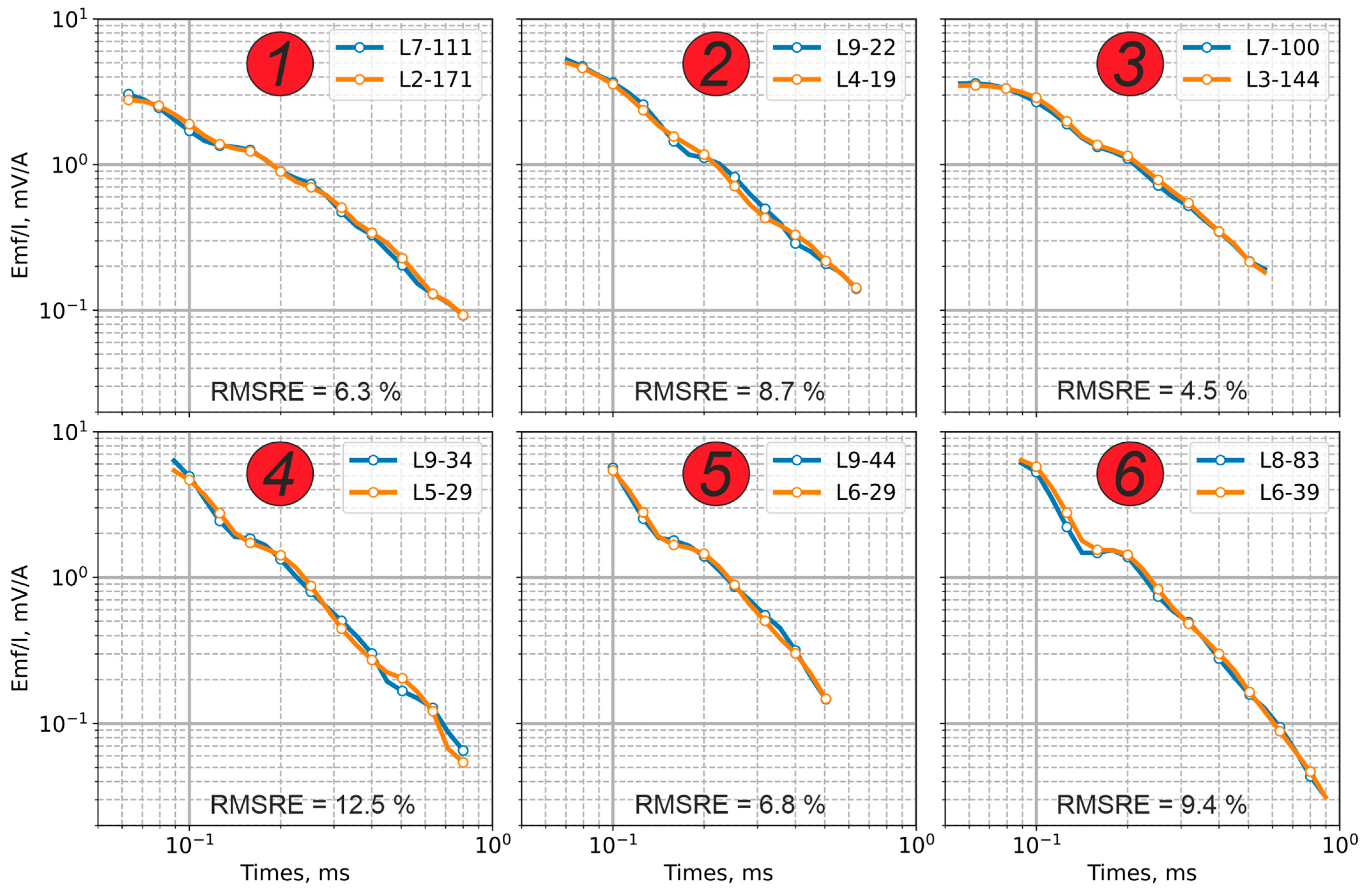
The total number of registered sounding curves was about 125,000. After the procedure described in the previous section, including robust data smoothing, the data were averaged over 1000 points with a step of 25 m between them. The measurements were conducted for several hours under adverse weather conditions, including a heavy snowstorm [https://youtu.be/rYpi5EfvVPQ (accessed on 6 November 2023)]. However, it was possible to collect data that were significantly better in quality than previous ones—our previous UAV-TEM system could measure transients down to 150 ns [2,8]. Due to the multiple increases in the frequency of samplings, up to 50 readings per second were now recorded. So, we had sufficient statistics to improve collected readings (stacking and removing noise). It allowed for an increased time range within the signals to be recorded confidently up to a time of 700–800 µs (Figure 4), which significantly increases the depth of investigation and accuracy of solving inverse problems.
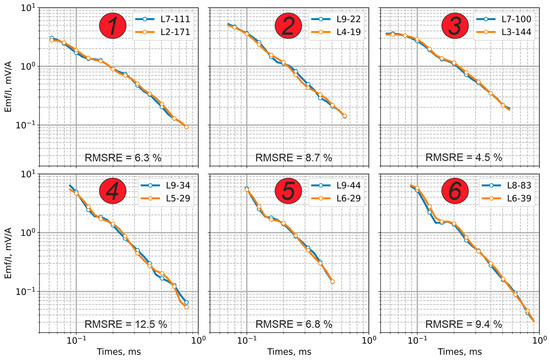
Figure 4.
Demonstration of high data quality: examples of assigned sounding curves and comparison of ordinary and control measurements. The locations of the measurements are shown in Figure 3b.
It is imperative to pay attention to the good coincidence of the sounding curves obtained at the coinciding points of intersecting profiles (Figure 4). Such points can be considered ordinary and control measurements. This clearly indicates the high quality of data obtained using the current version of the SibGIS UAV-TEM technology.
Indeed, at a flight speed of up to 35 km/h and a sampling rate of 50 readings per second, the density of observation points obtained using the UAV-TEM significantly exceeded that collected by standard helicopter survey at a flight speed of 120–150 km/h, and even more. The actual density of UAV-TEM observation points in practice reached point/10–point/25 m, which automatically created an advantage for solving inverse problems for areas with complex geological structures.
To quickly solve the inverse problem based on the obtained data and create a 3D model of electrical resistivity and geophysical sections, we applied a processing technique, first described in detail below.
3.1. UAV-TEM Data Processing: Modification of the Method of Calculation of Apparent Longitudinal Conductance S-tau
In the transition from ground-based soundings to airborne electromagnetic surveys, the issue of developing algorithms and calculating programs or software that provide efficient and fast interpretation of a huge amount of data, the amount of which can reach hundreds or even thousands of points per day, is of prime importance. We considered returning to the old and now largely forgotten method of differentially transforming EMF readings into curves of apparent longitudinal conductance as functions of time S(t) or depth S(H) and named the method S-tau (or Sτ). This method was proposed by Sidorov and Tikshaev at the end of the 1960s [11]. It became widespread in the 1970s and 1980s, but it is no longer used. The method’s main flaw was the unconditional identification of each local increase in longitudinal conductance S on the curve to the conductive layer and the non-increase part S(H) to the high-resistive rocks. Unfortunately, the authors and many users did not have enough knowledge about the theory of electromagnetic sounding, and the most enthusiastic, neglecting the laws of diffusion of EM fields in media, even tried to delineate more than ten layers of different resistivity at each TEM point. Alas, time, experience, and numerous boreholes have proved the inefficiency of the method when used for “high-resolution TEM”. Software for calculating multi-layer theoretical TEM curves that arrived in time pointed out to geophysicists the impossibility of the occurrence of local fluctuations on Sτ, which is a consequence of the diffusion processes of the propagation of EM fields in a real medium. In addition, induced polarization effects distorting the TEM readings have been discovered in many regions of the USSR and Canada, and their study has begun. Zadorozhnaya [12] showed that even a simple model composed of three conductive S-planes often cannot be unambiguously identified. Ageev [13] proposed that the fluctuations of the Sτ curves are mostly due to induced polarization processes occurring in rocks. Moreover, the numerical differentiation of the EMF readings itself can lead to fluctuations in the Sτ curves, which geophysicists identified as the presence of thin conductive layers in the section. Now, in the age of total computerization, most researchers use commercial software for the interpretation of TEM data based on solving direct problems of the distribution of the EM field in 1D or 2D models, and the Sτ-method has taken a back seat. However, even if we plan to perform 1D, 2D, or 3D inversions, it is necessary to speed up data processing—a quick qualitative assessment of the general structures in the investigated area is made. Then, an initial ‘starter’ model for inversion is chosen since, in this case, the inversion routine time can be reduced considerably. Thus, using the S-tau transformation, the authors managed to obtain very good results, for example, when interpreting airborne TEM data [7].
Having discarded the idea of ”high-resolution TEM”, the use of the method allows determining the conductance increasing with depth and determining the depth where Sτ increases noticeably. The presence of low-resistive objects (bodies and/or layers) in the section is associated with these parts of the curve S.
Consider the properties of conducting S-planes. Thin planes are also called Price’s sheets, Scheinman’s shits or S-planes. S.M. Scheinman (1947) [14] was the first to discuss the problem of transient processes induced by electrical and magnetic dipoles placed on a thin conductive layer. Scheinman formed special boundary conditions, which were obtained by limiting the transition from a thin layer to the S-plane as follows:
where h and σ are the thickness and conductivity of the layer, respectively. Sheinman’s solutions in the frequency domain are presented in the time domain using the integral Fourier transformation. Smythe V.R. (1950) [15] described the original solution derived from the method of imagining sources. He showed that the transient of an EM field can be presented as a so-called “floating plane” with longitudinal conductance S, i.e., the S-plane is moved (“floating”) from the source at a velocity of 1/μ S, where μ is magnetic permeability (μ = 4π10−7 H/m).
For the horizontal S-plane, the vector potential has only one component, Ax, and for an electrical line (dipole) AB, it is equal to:
where I is an electrical current (in amperes) and is a projection of the line connecting the point of observation to the coordinate plane. The Equation (2) completely coincides with the equation obtained by Sheinman (1947).
The equation for the vertical component of the magnetic field Bz can be presented as follows:
For a horizontal S-plane, the vector-potential has only one component Ax, so Equation (3) is simplified:
EMF in the receiving loop is calculated using Faraday law:
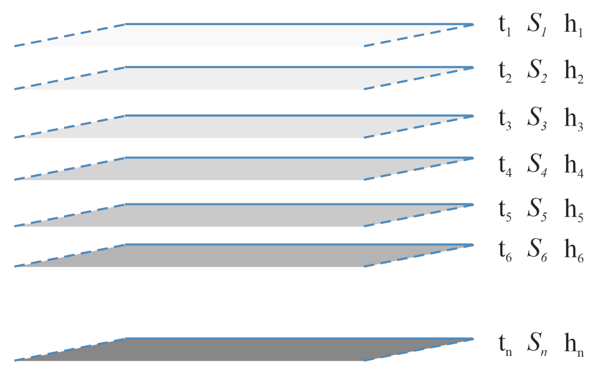
According to [15], regardless of the position of the observation point at each moment in time, the amplitude of the potential vector Ax and, accordingly, Bz and EMF (e(t)) will be equal to the amplitude of a certain “floating” conductive plane lying at a depth h(t) with conductance S(t), equivalent to the total longitudinal conductance of the entire section up to depth H = h(t) (Figure 5).
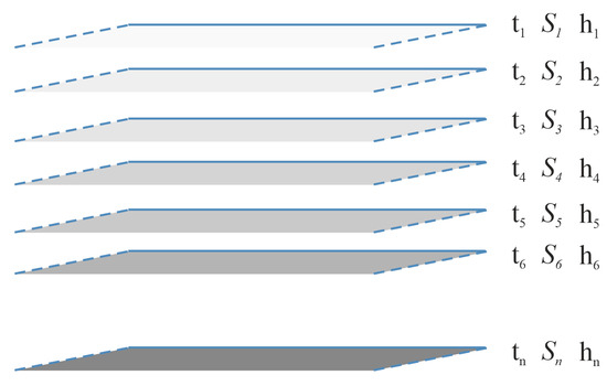
Figure 5.
Floating S-plane.
An increase in color tone indicates an increase in the conductance of the section with depth. When using in Equations (4) and (5), we obtain the formula EMF for “floating plane”:
where:
For airborne TEM, using a ground-based power source (a large loop or an electrical line) and a receiver loop suspended from the drone at the height z0:
Clearly, for the purposes of field data interpretation, the longitudinal conductance of the section at each point in time can be represented as the conductivity of a floating plane Sτ(H) located at a specific depth h(t):
However, for theoretical and field EM curves, it is impossible to determine the parameters of the “floating” plane using Equation (7) since that equation contains two unknown parameters, Sτ(H) and h(t), or more precisely, Sτ(t) and m(t). Thus, it is necessary to introduce a new function ϕ(m) that does not depend on S, namely:
The Equation (8) depends only on a certain parameter m, which is easily calculated for each time by comparing the calculated with the given function for the specified array. Now, substituting m(t) into Equation (7), we can calculate the longitudinal conductance of the section at a given point [11]:
Note that the method Sτ can only be used in the near zone of the source, that is, Kr ≪ 1, when (K is the wave number). Consider different types of theoretical curves Sτ(H). Let us first analyze the theoretical curves for two-layered models with the following parameters (Table 4). The theoretical EMF curves are calculated as follows. Given layered models with specified parameters of electrical resistivity ρi and thickness hi for each layer are used, then each layer is compressed into a thin plane Si [Equation (1)], and EMF are calculated in a model consisting of a set of S-planes.
Table 4.
Geoelectrical parameters of two-layered models located on the high resistive basement.
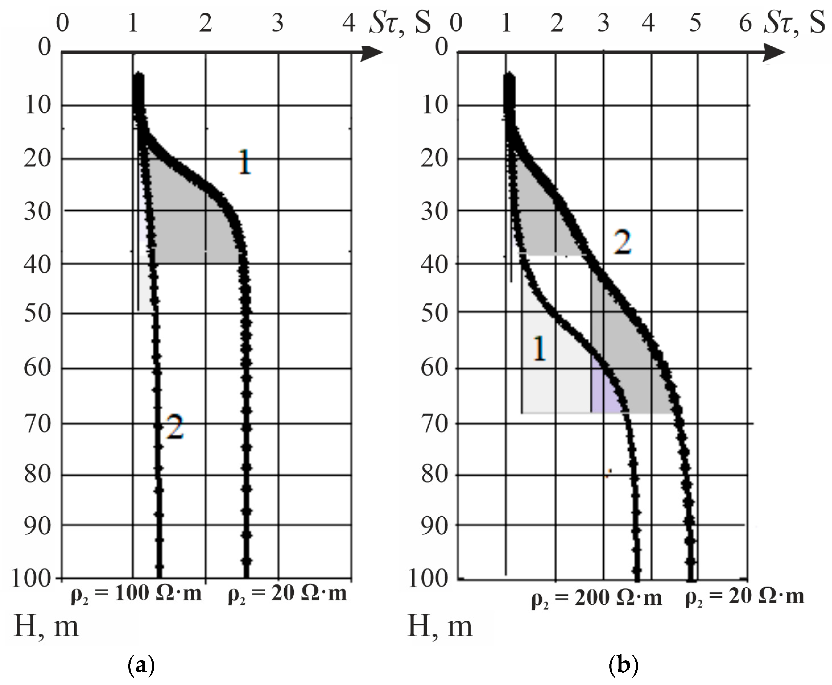
Figure 6a shows the curves Sτ(H) for two models where the intermediate layers have a resistivity of 20 and 100 Ω·m. In the case when the layer is more conductive, the longitudinal conductance increases sharply in the depth interval of 11 m to 38 m, which corresponds to the occurrence of this layer (curve 1). In the second case, the increase in conductivity from 1 S to 1.31 S occurs slowly (curve 2). However, even in this type of model, the presence of a layer with a resistivity of 100 Ω·m can be detected. The basement of the model (high restive halfspace) has no effect on the shape of the curves Sτ(H).
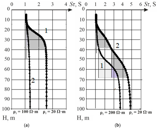
Figure 6.
Curves Sτ(H) for two (a) and four (b) layered models. The basement of both models is highly restive.
The geoelectrical parameters of two three-layer models are presented in Table 5. Figure 6b shows the curves Sτ(H) for these models.
Table 5.
Geoelectrical parameters of three layered models located on the high resistive basement.
In the first model, two conductive layers are separated by a rather thick layer (31 m) of high resistivity (200 Ω·m. In this case, the increase in longitudinal conductance due to the presence of the third conductive layer (15 Ω·m) shows up very clearly on the curves Sτ(H) at a depth of about 40 m (curve 1). If all three layers have low resistivity comparable in magnitude, then it is not possible to divide the curve Sτ(H) into parts corresponding to each layer (curve 2). Instead, we can see that the conductance of the model increases monotonically, and we are dealing with a highly conductive section or body in a certain depth interval. The blue lines show the surface of conductive layers (S-planes).
What is critical is that unless the EMF readings are distorted by induced polarization or/and superparamagnetic effects, the asymptotic branch of the curves Sτ always corresponds to the total conductance of the geological section.
As we can see, the method Sτ has some advantages. If there are conductive bodies and/or layers in the section, the use of this method makes it possible to trace the increase in longitudinal conductance Sτ(H) or Sτ(t) and to define the total conductance of the section SΣ at each TEM point. Furthermore, the calculation procedure is free of the principle of equivalence, which refers to the phenomenon in which one TEM curve can correspond to many geoelectric sections with radically different parameters (depths, number of layers, and resistivity).
3.2. Interpretation of Data
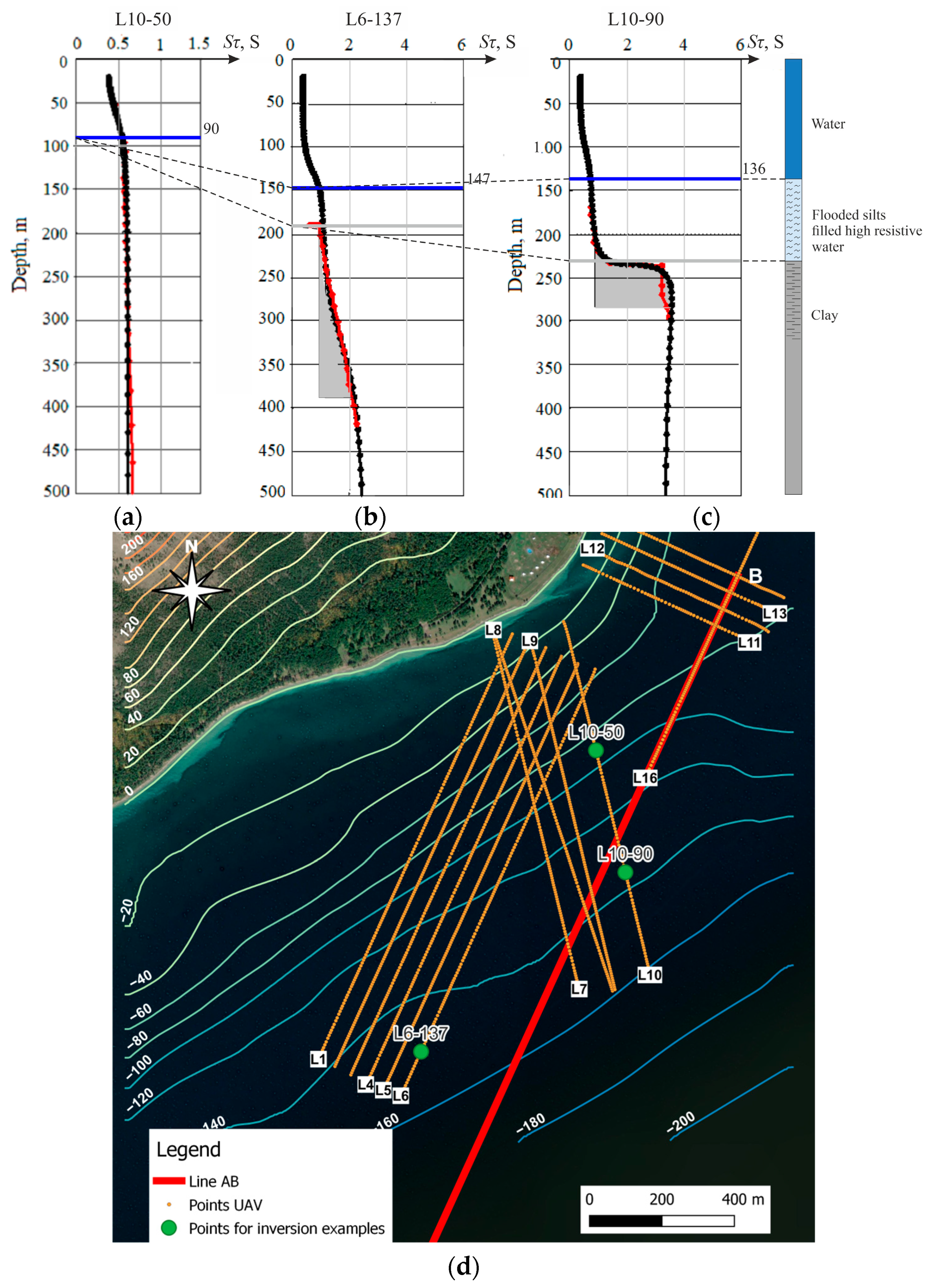
We transformed all EMF readings collected in the survey area into curves of apparent longitudinal conductivity. Three types of curves Sτ(H) were identified over the coastal part of Lake Baikal (Figure 7). For each curve, geoelectric models corresponding to the field curves were calculated. The parameters of the geoelectric sections are presented in Table 6.
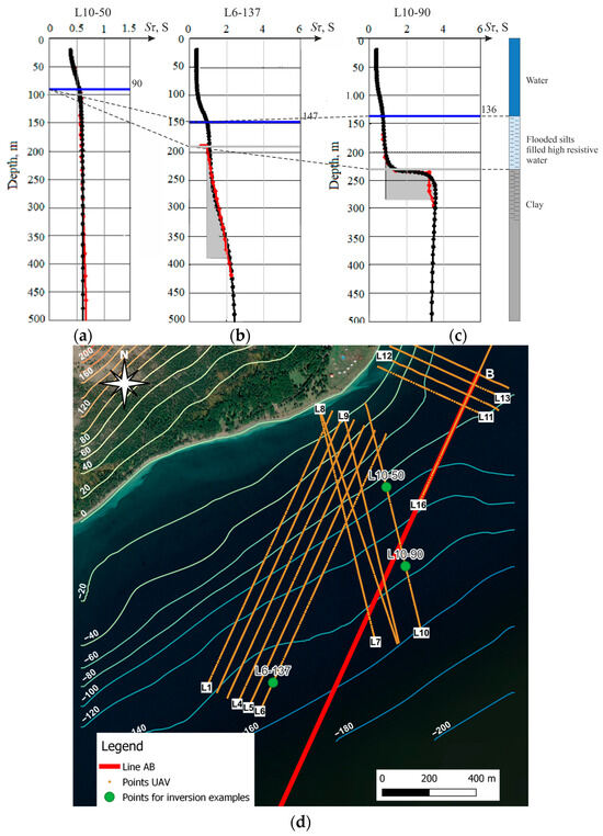
Figure 7.
Field and modeled curves Sτ(H). (a) Model 1 (profile 10, station 50), (b) model 2 (profile 6, station 137), (c) model 3 (profile 10, station 90), and (d) stations location. The surface of the bottom sediments is marked in blue.
Table 6.
Parameters of models corresponding to the points TEM.
Figure 7 shows the Sτ(H) curves of field data in red and theoretical Sτ(H) curves in black. Obviously, there is no information corresponding to the upper layer of water due to the impossibility of recording signals with the receiver MARS 2 at such early times. Therefore, data on the resistivity (110 Ω·m) of the first water layer are determined using mathematical modeling (Table 6). Figure 7a demonstrates Sτ(H) for the high resistive section where bottom sediments are absent. Curve Sτ(H) (Figure 7b) shows another type of high resistive section. For this type and also for type “c” (Figure 7c) at depths of 180 m and 215 m, there are bottom sediments with a resistivity of 160–180 Ω·m, represented by flooded silts. The increased resistivity of silt can be explained by its presence of unconsolidated or weakly consolidated rocks saturated with fresh water and extremely low mineralization. However, at these depths, there are no conditions for the formation of gas hydrates, and an increase in resistivity is evidenced by methane currents diffusing from deep layers into the water.
Model 3 shows the geoelectrical parameters acquired over low-resistive bottom sediments. A considerable increase in longitudinal conductivity caused by a layer with a resistivity of 40 Ω·m (about 1.875 S) is observed. There are sediments with higher longitudinal conductance (over 3 S) in the investigated area.
It is obvious that the parameters of the models fully correspond to the TEM data collected in nearby areas of Lake Baikal by a research team from SigmaGEO LLC (Irkutsk, Russia). In this area, the TEM instrument called ‘FastSnap’ has been tested in 2017. Several sounding curves have been recorded by “ground measurements on ice” [16]. Therefore, there are independent geoelectrical results. According to this survey, the area of the delta of the Goloustnaya River consists of three layers: lake water with a resistivity of about 160 Ω·m underlain by bottom sediments with a resistivity of about 60 and 20 Ω·m, which can include some ultra-low-and highly resistive units. According to our data, strata of conductive material with a resistivity of 10–50 Ω·m are located beneath the bottom sediments.
Analyses of curves show that the method Sτ reliably described the geoelectric parameters of the studied sections. Thus, the use of the Sτ method for the interpretation of airborne TEM data allows for obtaining models of the geoelectric sections that are quite close to real ones.
Since the position of the receiver Q in an airborne survey can be significant at a distance from AB, it will most likely correspond to the transition zone between the “near” and “far” zones. In this case, the method described above cannot be used. Therefore, it is necessary to modify this method for the large array being used. The sequence of the interpretation procedure is as follows:
1. Smoothing EMF readings. The readings in the interval of 50 μs–1.1 ms are mostly distorted by noises. In addition, in the vicinity of the AB line, powerful distortions are observed in the range of 110–190 ms. These distortions and noise were eliminated by logarithmic interpolation and smoothing.
2. Integration , calculation . The value of the vertical component of the magnetic induction depends only on the parameter m [Equation (4)]:
Thus, we transform the EMF readings into curves over the entire time interval:
Since the EMF curves are recorded over a limited time range, it is necessary to increase this interval until the contribution of the value of the integration element will be insignificant (at least up to 11 ms). Further, from the calculated total sum of elements , the elements are sequentially subtracted. The line AB is not a dipole and the integration is performed over all elements of , taking into account their distances and angles between as well as, the surface projection of the receiving loop.
3. The result of the integration [Equation (11)] can be verified by the differentiation of with respect to t [Equation (5)].
4. Smoothing curves .
5. Finding at each sounding. At each time for the given parameters of the array, we ensure the coincidence of the transformed and the theoretical curves and determine . At this stage, in fact, we still do not know either the electrical conductance of the effective S-plane or its depth.
6. Now, for a given function , we calculate the theoretical curve for a new array, which means for a small loop-in-loop configuration (AB = 50 m, R = 25 m) located on the ground (z0 = 0).
7. Differentiating the theoretical with respect to the time t we obtain for a new array. Such theoretical curves allow us to apply the method to each TEM reading.
8. Smoothing of the signals.
9. Calculation Sτ(H) as described above [11] [Equation (11)].
10. Smoothing Sτ(H).
11. The depth of the “floating” plane can be calibrated using available drilling data (in our case, there are bathymetry data of the Bolshoe Goloustnoe site of Lake Baikal). Depending on the distance from the AB line, the depth is calculated as
12. Visualization of Sτ(H) along profiles (2D) and over the entire area (3D).
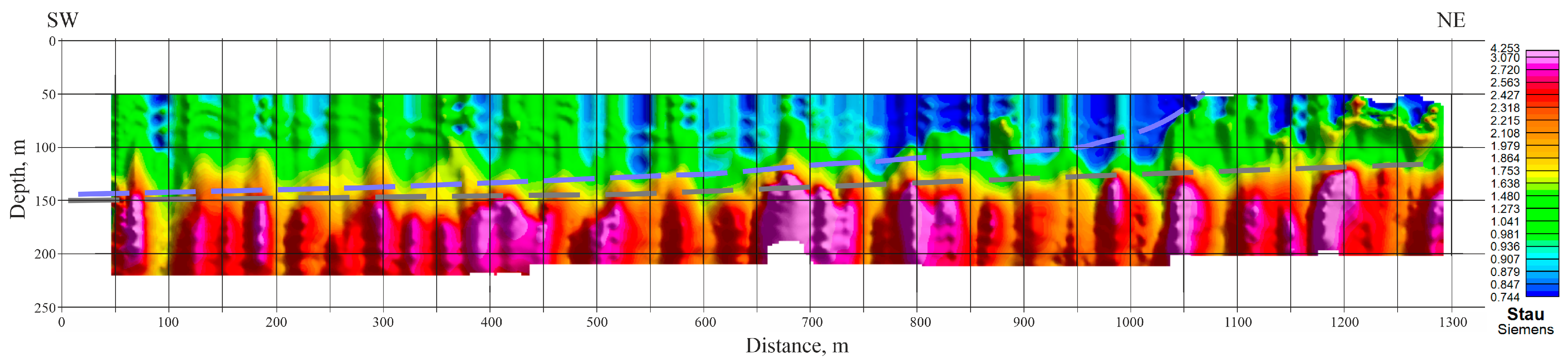
Each reading was transformed into apparent longitudinal conductance Sτ(H). An example of a cross-section of Sτ(H) for profiles 2 and 6 is shown in Figure 8 and Figure 9. The sections clearly show a high-resistivity layer corresponding to Baikal water and sedimentary deposits characterized by low resistivity. High resistivity bottom silt and clayey sediments cannot be distinguished on the Sτ(H) curves as two separate layers. In this case, both layers appeared as a single weak conductor (Curve 2, Figure 7). If the electrical conductivity of clays is low, eddy currents are concentrated in this layer. The information on the bottom silt layer can only be obtained using mathematical modeling data. A comparison of the Sτ(H) along profiles 2 and 6 shows an excellent correlation between the main blocks of the section. On the right side of the profiles, the apparent longitudinal conductance of the water increases due to the inflow of contaminant materials brought from the shore by wind and Goloustnaye River flow.
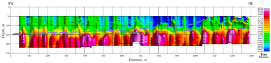
Figure 8.
Apparent longitudinal conductance Sτ(H) along profile L2 (closer to the coast). Light blue dashed lines indicate the interface between water and flooded silts. Gray dashed lines indicate the interface between flooded silts and conductive clays. Visualization in Oasis Montaj.

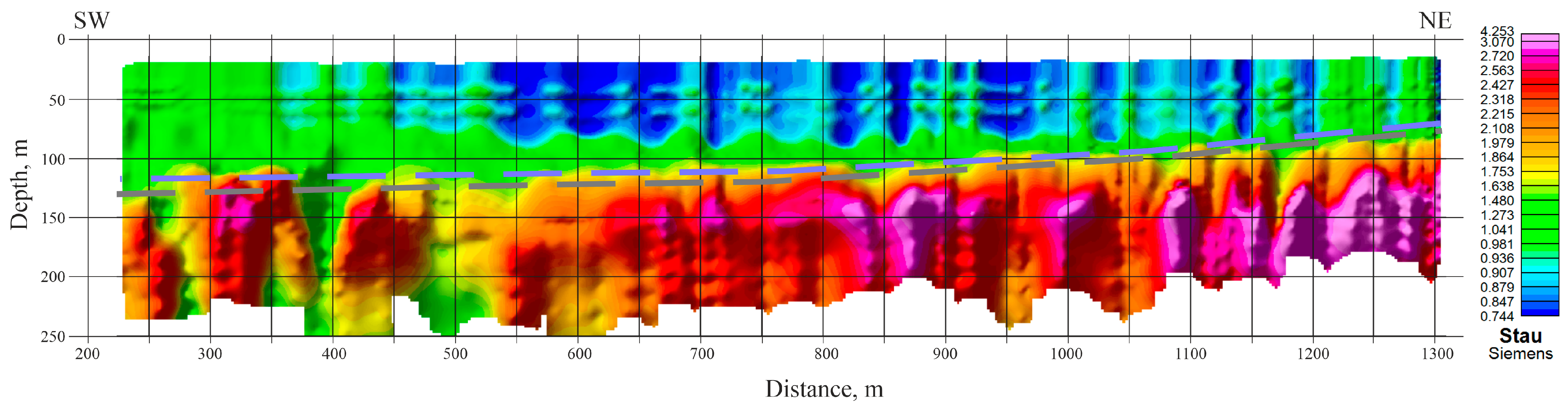
Figure 9.
Apparent longitudinal conductance Sτ(H) along profile L6 (closer to the AB line). The legend is shown in Figure 8. Visualization in Oasis Montaj.
In the center of the profiles, the longitudinal conductance of water decreases, but at the ends of the profiles (left western part), the depth of the lake increases and, accordingly, increases the conductance of the water layer. Unfortunately, it is not possible to determine the exact thickness of the water since the electromagnetic field in high-resistive materials propagates at a high velocity . This fact does not interfere with studying the structure of underlying sedimentary deposits.
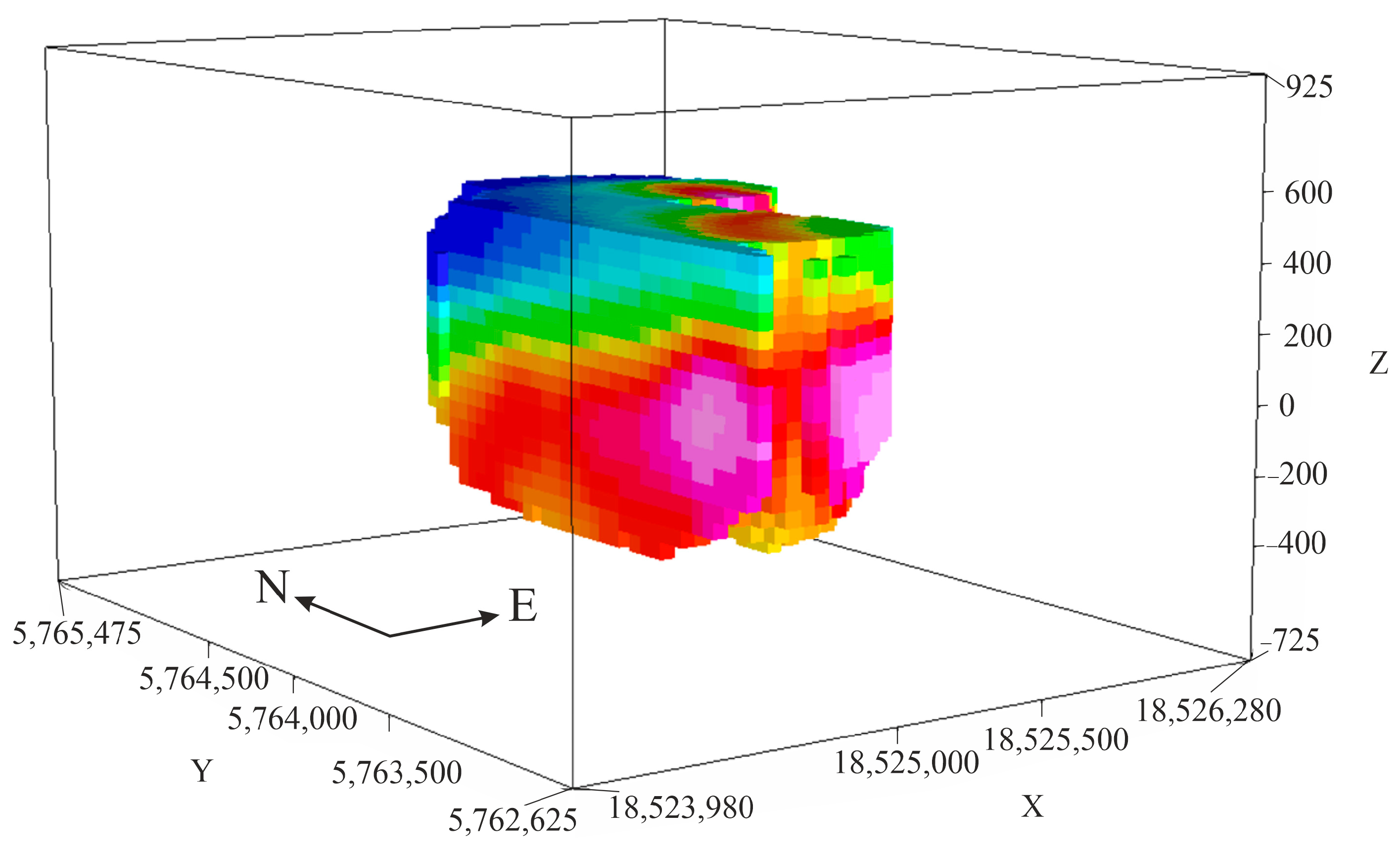
A sufficiently dense network of profiles made it possible to present a 3D visualization of the TEM data using the model of a “floating” plane. Figure 10 and Figure 11 demonstrate a 3D geoelectrical model of the survey area with the topography of the coastal zone. The isolines of the bottom area are applied to it. The 3D geoelectrical model demonstrates an excellent correlation of high-resistive and low-resistive blocks not only along the profiles but also over the area. The results show that high-resistance objects stand out under the water layer of 100–220 m in conductive sediments to a depth of at least 200 m. In these areas, the apparent electrical conductivity of the underwater section decreases to zero, and the total conductivity of the soundings is determined only by the electrical conductivity of the lake water. The revealed block of high resistance is a continuation of the release of indigenous metamorphosed Proterozoic age rocks. This block can be traced on the map of the total longitudinal conductivity of the bottom sediments in the studied area (Figure 12). On the top of the ground, the green line of the echelon fault runs along the crest of the hill through a probable seismic dislocation and reflects shear deformation within the zone of influence of the coastal fault, which can be traced deep into the lake.

Figure 10.
Geophysical section based on a 3D model, showing the structure of the water and rocks from the shore to depth. The legend is shown in Figure 8. Visualization in Voxler.
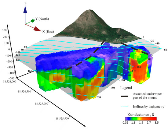
Figure 11.
Apparent longitudinal conductance Sτ(H) along profile 6 (closer to the AB line). Visualization in Voxler.
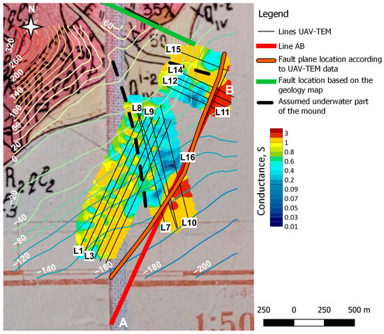
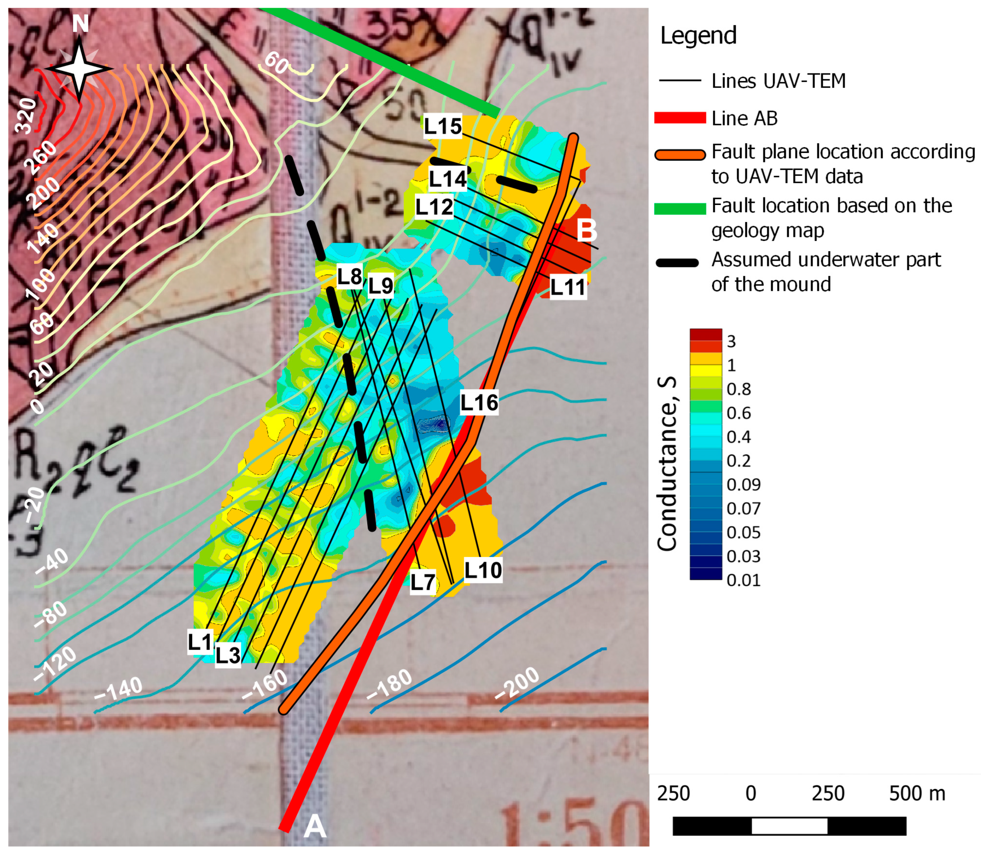
Figure 12.
Map of the total longitudinal conductance of bottom sediments. Visualization in QGIS.
Outside of high-resistance blocks, the conduction of the lacustrine sediments increases with depth. The distribution of the electrical conductivity of these coastal sediments is mosaic in nature with a conductivity of 0.3–3 cm, probably due to the presence of coarse-grained material.
The presence of local high-resistive inclusions in the bottom sediments at a depth of 450–500 m down to 100 m may be regarded as lenses of gas hydrates, which were repeatedly observed in Baikal during expeditions of the Limnological Institute of the Siberian Branch of the Russian Academy of Sciences [17,18].
The zone of abrupt transition from a zone of low electrical conductivity in the left part to a zone of high conductivity in the right part is caused by a coastal fault with a system of discharges. The approximate location of this fault is shown in Figure 12 with an orange dotted line.
Thus, the data obtained do not contradict the results of previous works but complement them.
4. Conclusions
An unmanned aerial system was used to conduct a TEM survey on the Lake Baikal coast. The transmitter CTU-HV was used as a current pulse generator. Current pulses were induced in an electrical line 2.2 km long. The iron poles were lowered into the ice holes. The receiver and the multi-turn inductive sensor with an effective area of 2500 m2 were suspended from the drone on a cable. The soundings were carried out along 16 profiles, and the total number of soundings was more than 125,000. As a result, high-quality sounding curves were obtained for times up to 700 μs–1 ms, suitable for qualitative and quantitative interpretation. It is shown that the quality of the data has increased significantly compared to the first version of the SibGIS UAV-TEM system of the 2020 model. The actual sounding depth was more than 400 m.
For fast interpretation, we used a modified Stau method, which makes it possible to calculate the apparent longitudinal conductance as a function of depth at each sounding point. Thanks to this, it became possible to process data and obtain the start models of the geological structure of the study area in a time comparable to the time of fieldwork, whereas the software we previously used for 1D inversion did not allow us to obtain results on such a volume of data faster than in 1–2 months, which significantly reduced the effect of using UAV-MPP instead of a ground survey. The Stau inversion technique is described in detail in the article.
The modified inversion for UAV-TEM data has proven to be effective in lateral differentiation in the upper part of the sedimentary material covered by more than 100–200 m of freshwater sediments, as well as in identifying high resistive structures. As a result of the research, data were obtained that were fundamentally similar to single measurements of predecessors. However, thanks to a significantly larger volume of geoelectrical surveys, new information was obtained about the geological structure of Lake Baikal in the area of the Bolshaya Goloustnaya River.
The high-resistivity cone-shaped mound is composed of coarse-clastic alluvial sediments lying on a bedrock of metamorphosed Proterozoic age rocks and can be clearly identified.
Another type of section is presented in a significant portion of the coastal area. In this type, high-resistivity clastic bottom sediments are underlain by low-resistivity clayey lacustrine deposits. With an increase in the depth of the lake, the sediments of the alluvial cone wedge out, the thickness of clayey lacustrine sediments increases to hundreds of meters, and high lenses with a high content of methane appear in the upper part of the section. The obtained materials can be considered as evidence in favor of confirming the hypothesis about the presence of gas hydrate deposits in this area [17,18] since electrical prospecting data can be interpreted as the presence of a methane flow leads to the formation of high-resistivity lenses of gas hydrates at a depth of 450–500 m.
Thus, it is shown that at the current level of UAV-TEM technology, including both the hardware, the methods, and the data processing environment, in contrast to its earlier version, can already be fully considered a solution that allows replacing traditional surveys while being significantly superior them in terms of productivity. However, this case also allowed us to record a number of shortcomings that will be corrected in the future:
Using the Stau method, it is not possible to accurately determine the thickness of the water due to its high resistivity. This is especially noticeable at shallow depths in the coastal part (Figure 10 and Figure 11). This problem is typical for any cuts with high top resistance.
Because the range of a confidently measured signal is quite narrow, either the moment of the electric line (current and length) and/or the effective moment of the receiver loop Q must be increased.
Noise, instrumental interferences, and geological distortions make it difficult to develop software for automated interpretation, especially when the TEM profile crosses the electrical transmitter line. To optimize the interpretation process, it is recommended to place the sounding profiles parallel to and away from the current (transmitter) line.
We believe that the presented material convincingly demonstrates that the Stau transformation allows us to significantly optimize UAV-based electromagnetic prospecting. It is shown that geoelectrical models we obtain from the results of Stud transformation can be valuable not only as rough starting models for 1D and 3D inversion but can also be quite suitable for geological interpretation.
5. Patents
SibGIS Tech LLC.; Parshin, A. Aeroelectric prospecting method using lightweight unmanned aerial vehicle. RU Patent 2736956 C1, 9 January 2020.
Author Contributions
Conceptualization, Y.D. and A.P.; methodology, V.H.-Z. and A.P.; software, V.H.-Z. and A.B.; validation, Y.D. and V.H.-Z.; investigation, A.P., A.B. and V.H.-Z.; data curation, A.B. and V.H.-Z.; writing—original draft preparation, V.H.-Z. and A.P.; writing—review and editing, A.P.; visualization, A.B. and V.H.-Z.; supervision, A.P.; project administration, Y.D. and A.P.; funding acquisition, A.P. and Y.D. All authors have read and agreed to the published version of the manuscript.
Funding
This research was funded by RSCF (grant No. 20-67-47037).
Data Availability Statement
Data available on request.
Conflicts of Interest
The authors declare no conflict of interest.
References
- Persova, M.G.; Soloveichik, Y.G.; Vagin, D.V.; Kiselev, D.S.; Sivenkova, A.P.; Simon, E.I. Resolution Analysis of Airborne Electromagnetic Survey Using Helicopter Platform and UAV. In Proceedings of the 2021 XV International Scientific-Technical Conference on Actual Problems of Electronic Instrument Engineering (APEIE), Novosibirsk, Russian Federation, 19–21 November 2021; pp. 591–594. [Google Scholar] [CrossRef]
- Parshin, A.; Bashkeev, A.; Davidenko, Y.; Persova, M.; Iakovlev, S.; Bukhalov, S.; Grebenkin, N.; Tokareva, M. Lightweight Unmanned Aerial System for Time-Domain Electromagnetic Prospecting—The Next Stage in Applied UAV-Geophysics. Appl. Sci. 2021, 11, 2060. [Google Scholar] [CrossRef]
- Kotowski, P.O.; Becken, M.; Thiede, A.; Schmidt, V.; Schmalzl, J.; Ueding, S.; Klingen, S. Evaluation of a Semi-Airborne Electromagnetic Survey Based on a Multicopter Aircraft System. Geosciences 2022, 12, 26. [Google Scholar] [CrossRef]
- Stoll, J.; Noellenburg, R.; Kordes, T.; Becken, M.; Tezkan, B.; Yogeshwar, P.; Bergers, R.; Matzander, U. Semi-Airborne electromagnetics using a multicopter. In Proceedings of the International Workshop on Gravity, Electrical & Magnetic Methods and Their Applications, Xi’an, China, 19–22 May 2019. [Google Scholar]
- Vilhelmsen, T.B.; Døssing, A. Drone-towed CSEM system for near-surface geophysical prospecting: On instrument noise, temperature drift, transmission frequency and survey setup. EGUsphere, 2022; in preprint. [Google Scholar] [CrossRef]
- Smit, J.; Stettler, E.; Price, A.; Schaefer, M.; Schodlok, M.; Zhang, R. Use of drones in acquiring B-field total-field electromagnetic data for mineral exploration. Miner. Econ. 2022, 35, 455–465. [Google Scholar] [CrossRef]
- Zadorozhnaya, V.; Stettler, E. The use of the ‘‘floating’’ S-plane for effective interpretation of airborne TEM data. In Proceedings of the EM Induction Workshop, Çeşme, Turkey, 11–17 September 2022. [Google Scholar]
- Parshin, A.; Davidenko, Y.; Yakovlev, S.; Vinokurov, V.; Bashkeev, A. Lightweight TEM and VLF systems for low-altitude UAV-based geophysical prospecting. In Proceedings of the NSG2021 27th European Meeting of Environmental and Engineering Geophysics Conference Proceedings, Bordeaux, France, 2 September 2021; Volume 2021, pp. 1–5. [Google Scholar]
- Zaharkin, A.K. Compact receiving loop for pulsed electrical prospecting. Ross. Geofiz. Zhurnal 1998, 9–10, 95–99. (In Russian) [Google Scholar]
- Parshin, A.; Budyak, A.; Chebokchinov, I.; Sapunov, V.; Bulnayev, A.; Morozov, V. Complex UAS-Geophysical Surveys at the First Stages of Geological Prospecting: Case in the Western Sayan (Russia). In Proceedings of the First EAGE Workshop on Unmanned Aerial Vehicles Extended Abstracts, Tolouse, France, 2–4 December 2019. MoUAV02. [Google Scholar]
- Sidorov, V.; Tikshaev, V. Interpretation of transient electromagnetic signals registered in near zone. Razvedochnaya Geofiz. 1970, 42, 45–54. (In Russian) [Google Scholar]
- Zadorozhnaya, V.Y. Interpretation of TDEM for Search of Bioherms in the Pre-Caspian Depression. Ph.D. Thesis, All-USSR Geophysical Institute, Moscow, Russian, 1984. (In Russian). [Google Scholar]
- Ageev, V.V. Mathematical Modeling of Electromagnetic Soundings of Polarizing Media and the Problem of High-Resolution Electrical Exploration. Ph.D. Thesis, IGEMI, Moscow, Russian, 1977. (In Russian). [Google Scholar]
- Sheinman, S.M. On the transient of electromagnetic fields in the Earth. Prikl. Gofizika 1947, 3, 3–55. (In Russian) [Google Scholar]
- Smythe, V.R. Static and Dynamic Electricity, 2nd ed.; McGRAW HILL BOOK COMPANY Inc.: New York, NY, USA, 1950; p. 637. [Google Scholar]
- Sharlov, M.V.; Kozhevnikov, N.O.; Sharlov, R.V. Lake Baikal—A Unique Site for testing and calibration of near-surface TEM systems. In Proceedings of the 23rd European Meeting of Environmental and Engineering Geophysics, Malmö, Sweden, 3–7 September 2017. [Google Scholar] [CrossRef]
- Khlystov, O.; De Batist, M.; Shoji, H.; Hachikubo, A.; Nishio, S.; Naudts, L.; Poort, J.; Khabuev, A.; Belousov, O.; Manakov, A.; et al. Gas hydrate of Lake Baikal: Discovery and varieties. J. Asian Earth Sci. 2013, 62, 162–166. [Google Scholar] [CrossRef]
- Khlystov, O.M.; Nishio, S.H.; Manakov, A.Y.; Sugiyama, H.; Khabuev, A.V.; Belousov, O.V.; Grachev, M.A. The experience of mapping of Baikal subsurface gas hydrates and gas recovery. Russ. Geol. Geophys. 2014, 55, 1122–1129. [Google Scholar] [CrossRef]

Disclaimer/Publisher’s Note: The statements, opinions and data contained in all publications are solely those of the individual author(s) and contributor(s) and not of MDPI and/or the editor(s). MDPI and/or the editor(s) disclaim responsibility for any injury to people or property resulting from any ideas, methods, instructions or products referred to in the content. |
© 2023 by the authors. Licensee MDPI, Basel, Switzerland. This article is an open access article distributed under the terms and conditions of the Creative Commons Attribution (CC BY) license (https://creativecommons.org/licenses/by/4.0/).