A Multiple Agile Satellite Staring Observation Mission Planning Method for Dense Regions

Abstract

To fully harness the burgeoning array of in-orbit satellite resources and augment the efficacy of dynamic surveillance of densely clustered terrestrial targets, this paper delineates the following methodologies. Initially, we leverage the Density-Based Spatial Clustering of Applications with Noise (DBSCAN) clustering algorithm to aggregate the concentrated terrestrial targets, taking into account the field-of-view peculiarities of agile staring satellites. Subsequently, we architect a model for a synergistic multiple angle earth observation satellites (AEOSs) mission planning with the optimization objectives of observational revenue, minimal energy expenditure, and load balancing, factoring in constraints such as target visibility time window, AEOSs maneuverability, and satellite storage. To tackle this predicament, we propose an improved heuristic ant colony optimization (ACO) algorithm, utilizing the task interval, task priority, and the length of time a task can start observation as heuristic information. Furthermore, we incorporate the notion of the max–min ant system to regulate the magnitude of pheromone concentration, and we amalgamate global and local pheromone update strategies to expedite the convergence rate of the algorithm. We also introduce the Lévy flight improved pheromone evaporation coefficient to bolster the algorithm’s capacity to evade local optima. Ultimately, through a series of simulation experiments, we substantiate the significant performance improvements achieved by the improved heuristic ant colony algorithm compared to the standard ant colony algorithm. We furnish proof of its efficacy in resolving the planning of multiple AEOS staring observation missions.

1. Introduction

As the realm of space science and technology burgeons, the mission demands for terrestrial observation intensify in complexity. A single satellite operating in the conventional scanning mode proves insufficient for fulfilling intricate observational demands, and the relationships among satellites are in a state of rapid flux [1]. Consequently, the comprehensive coordination of satellite resources, the fulfillment of user necessities, and the integration of multifarious constraints such as target distribution traits and satellite attitude maneuver characteristics for dynamic terrestrial target surveillance, optimal mission planning, and the maximization of satellite resource benefits have emerged as pressing issues in the field of remote sensing. The optimal resolution of these issues presents a formidable challenge for the on-orbit application of multiple AEOSs. Presently, instances of cooperative multi-satellite operations have been observed, including NASA and JAXA’s deployment of the GPM mission [2], the German commercial satellite constellation RapidEye [3], the EU’s QB50 mission [4], and the Chinese Beidou satellite [5].

Agile optical satellites, equipped with specialized equipment, execute a myriad of observational assignments. The operational modes primarily employed by these celestial instruments include scanning mode and staring mode. In the scanning mode, a continuous surveillance and data acquisition of the target is accomplished by propelling the sensor in a designated direction, making this mode particularly beneficial for expansive remote sensing imagery, large-scale mapping, and analogous applications. The mission planning for scanning mode predominantly revolves around the striping of the target zone and the sequencing of observation, among other factors. Conversely, staring mode is utilized in high-stakes operations such as dynamic monitoring, counter-terrorism initiatives, and disaster mitigation efforts. In this mode, the sensors remain static, perpetually observing the same region for a specified span. Unlike the scanning mode, the staring mode necessitates considerations of mission duration constraints and is not reliant on the satellite’s motion direction during imaging [6]. Moreover, staring mode offers a superior degree of adaptability in mission planning. As a burgeoning optical imaging mode, staring mode is aptly suited for enabling dynamic and prolonged surveillance of targets in densely regions.

In the realm of AEOSs’ mission planning in scanning mode, early scholarly pursuits such as those cited in literature [7], proposed solution methodologies, encompassing the greedy algorithm, dynamic planning algorithm, constraint planning algorithm, and local search algorithm for the scheduling model of AEOSs. Habet [8] introduced a tabu search algorithm to enhance the solution’s quality by introducing and resolving a secondary issue, employing a dynamic programming algorithm to solve the relaxation problem’s upper bound. Xu [9] utilized a priority-based sequential construction process to circumvent conflicts and generate viable solutions, thereby reducing the complexity of feasibility verification and corroborating the algorithm’s efficacy. Additionally, Mok [10] suggested a straightforward yet effective heuristic mission planning approach for this issue, augmenting the image count by introducing additional degrees of freedom on the pitch axis, albeit at the cost of potentially compromising solutions quality due to increased running speed. Qiu [11] employed a traditional simulated annealing algorithm to address the problem, considering directional inversion and integration time accumulation in scanning imaging. Du [12] proposed an improved ant colony algorithm founded on perception and awareness strategies to resolve the polygon region observation problem, yielding more substantial results than the traditional ant colony algorithm. Concerning mission planning in staring mode, Yu [13] proposed a scheduling model incorporating specified observation and revisit time and devised a cooperative-oriented ant colony optimization algorithm to determine each satellite’s observation sequence. However, the algorithm only accounted for maximal observation gain, neglecting the energy expenditure during satellite maneuvers and inter-satellite load balancing. Cui [14] designed an improved ant colony algorithm with a tabu list, significantly boosting the algorithm’s efficiency. However, the algorithm only considered a singular satellite scenario, neglecting the satellite’s onboard resource constraint, rendering it impractical for real-world applications. Ji [15] proposed a region partitioning method and a residual time allocation method to maximize each subregion’s observation staring duration, employing a path inference strategy to achieve the observation path of multiple satellites. However, the paper overlooked the satellite’s resource usage. In the above-mentioned article, when continuously observing adjacent mission points, the satellite’s attitude transition time was assumed to be independent of its actual position, treating it as a constant value. For low earth orbit satellites, the attitude transition time is contingent upon the satellite’s attitude moment, the rotational axis’s angular velocity, and the angular acceleration, among other attributes, which cannot be simply set. In observing regional dense point targets, due to the close mission distance, only one mission is observed in one maneuver, leading to frequent maneuvers of the satellite and significant wastage of satellite resources, necessitating the consideration of target point synthesis. While the study of mission clustering in scanning mode is relatively mature, it is challenging to directly apply the clustering method from scanning mode to staring mode, as the mission planning constraints in the staring mode differ from those in the scanning mode.

Collaborative mission planning for multiple Agile Earth Observing Satellites (AEOSs) presents a highly intricate and combinatorial optimization challenge, offering multiple options across various dimensions. As an extension of single satellite mission planning, it is logical to adapt existing heuristic algorithms for single satellite mission planning to address multi-satellite mission planning. Numerous studies have been conducted on single satellite mission planning, with literature [10,11,14] primarily focusing on this topic, while literature [12,13,15] has focused on multi-satellite mission planning problems. Vasquez [16] introduced a tabu search algorithm based on the French satellite Spot, examining its optimal scheduling. Xhafa [17] conducted an optimal scheduling study for a single satellite using a genetic algorithm for ground station scheduling in a specific scenario. Tangpattanakul [18] proposed an indicator-based multi-objective local optimization algorithm for resolving single satellite multi-objective optimization challenges. Song [19] proposed a clustering-based genetic algorithm (C-BGA) for the satellite ranging scheduling problem using the k-means clustering method. Liu [20] suggested an adaptive large-neighborhood search algorithm to address the single satellite scheduling problem and established a conflict-free timeline. Long [21] implemented a two-phase process of mission clustering and planning, utilizing an improved graph-theoretic cluster partitioning algorithm along with a hybrid genetic and simulated annealing (GA-SA) algorithm to augment its optimization capability. Lu [22] presented a unified description for different types of targets and utilized an improved particle swarm algorithm to solve the mission planning model. However, these studies are only applicable to planning and scheduling for a single satellite and cannot manage large-scale mission planning problems. Bianchessi [23] proposed a tabu search heuristic algorithm considering multiple satellites with multiple orbits, using column generation techniques to obtain upper bounds on the gains. Kebin [24] suggested a hybrid ant colony optimization algorithm, combining an iterative local search algorithm to generate high-quality multi-satellite observation schedules. For the Earth Electromagnetic Satellite Scheduling Problem (EESSP), a Learning Adaptive Genetic Algorithm (LA-GA) has been proposed in the literature [25] to solve the problem. For the multi-satellite mission planning problem of large area mapping, Chen [26] proposed a multi-objective modeling approach, utilizing a non-dominated ranking genetic algorithm to solve the model, while employing the Vatti algorithm to enhance solution efficiency. Liu [27] introduced a Q-network-based network scheme to address the single-satellite scheduling problem, using a profit-based competition strategy to enhance the multi-satellite mission planning system efficiency. Deng [28] suggested a neural network-based multi-grain negotiation method under a decentralized structure with a low cost–benefit ratio for mission assignment and planning of microsatellite clusters. Song [29,30] combined reinforcement learning-assisted genetic algorithms to efficiently solve the satellite scheduling problem. He [31] suggested an inference-based agile satellite scheduling method for solving the coupling within each satellite subsystem. However, most of these studies do not simultaneously consider the attitude time, the energy consumption of attitude maneuvers, and the on-satellite resource usage of the satellite when performing two adjacent missions in the mission planning modeling process. Therefore, these methods pose challenges when applied in practical mission planning.

To efficiently address the task planning problem for dense area targets in the context of multiple AEOSs staring observation mode, we still need to solve the following three issues:

• Traditional clustering methods used in the scanning observation mode cannot be directly applied to the emerging staring observation mode. This is because the rectangular field of view constraint in the staring mode is more stringent and demanding compared to the strip field of view constraint in the scanning mode. Additionally, in staring imaging, the imaging is not constrained by the motion direction during the imaging of the Earth’s surface, allowing for more flexible maneuverability.
• In the current research, the assumption is made that the satellite’s attitude transition time is independent of the satellite’s actual position and is considered constant. However, in reality, the attitude transition time depends on various factors such as the attitude torque of the satellite, the angular velocity of the axes, and the angular acceleration. When performing transitions for Earth observation tasks, it is not appropriate to simply set a fixed value for the attitude transition time. These factors need to be taken into account to accurately model the attitude transition time during the task transitions.
• In the current mission planning and modeling process, the simultaneous consideration of satellite’s attitude transition time, energy consumption during attitude maneuvers, and balanced utilization of on-board resources between adjacent tasks is lacking. This incomplete modeling approach may not be conducive to practical applications. To achieve more accurate mission planning, it is necessary to comprehensively consider these factors and ensure efficient utilization of resources and energy during task execution. This will help improve the efficiency and performance of task execution.

Based on the research analysis and the existing problems, we have designed a DBSCAN clustering algorithm based on the satellite’s field of view and an improved ant colony algorithm. Firstly, the point targets in the scene are clustered based on the size of the satellite payload’s field of view to reduce the number of satellite axis maneuvers and minimize the consumption of on-board resources. Secondly, we have designed an improved ant colony algorithm to plan the observed target points after clustering. This algorithm incorporates heuristic information such as task interval time, task priority, and task start time length, and combines the idea of a maximum–minimum ant system to limit the concentration of pheromones. It uses global and local pheromone update strategies to improve the convergence speed of the algorithm. Additionally, a Levy flight is introduced to enhance the algorithm’s ability to escape local optima by improving the pheromone evaporation coefficient. Finally, the effectiveness and rationality of the proposed algorithm are validated through simulation experiments and compared with the standard ant colony algorithm.

The remainder of this paper unfolds as follows. Section 2 elucidates the process of modeling AEOS mission planning within the purview of staring observation mode, encapsulating aspects such as target clustering, model presuppositions, and model development, whilst offering methods for clustering and model resolution. In Section 3, we delineate the experiments executed with a trio of satellites and 180 densely packed target points, aimed at discovering the optimal algorithmic parameters, and conduct a comparative analysis to underscore the superiority of the improved heuristic ant colony algorithm proposed herein, against the standard ant colony algorithm. The proposed methodology is deliberated upon in Section 4. Finally, Section 5 imparts the conclusions drawn from the study.

2. Materials and Methods

Given that the instantaneous field of view of an agile Earth observation satellite operating in the staring observation mode can encompass multiple targets, the efficiency of observation can be significantly augmented by judiciously clustering these targets into a collective, prior to satellite mission planning. This paper, therefore, clusters the target points in accordance with the satellite’s field of view.

2.1. Target Clustering in Staring Observation Mode

2.1.1. Clustering Model Construction

The dimensions of the satellite’s field of view are dictated by the conjunction of the satellite’s orbital altitude and the observational angle of the visible camera. The consideration of the satellite’s field of view in this paper is limited to the minimal coverage area when the satellite is in a nadir-looking position, disregarding any potential alterations in coverage due to satellite angle, thus adopting a somewhat conservative approach.

Assuming that the satellite orbit is a circular orbit, with the earth’s radius denoted as $R_e$, the orbital radius as $R_s$, and the field of view for the satellite’s optical payload as $\varphi$, it should be noted that clustering conditions exhibit variation in line with the differing shapes of the optical payload’s field of view. In this treatise, we posit that a square field of view shape, with the terrestrial coverage of the satellite, is shown schematically in Figure 1:

As gleaned from Figure 1, the satellite’s ground coverage is influenced by both its orbital altitude and the optical payload’s field of view. Therefore, the edge length l of terrestrial coverage, as delineated by the satellite’s field of view, is expounded by Equation (1):

$$l=2(R_s-R_e)tan\left(\frac{\varphi }{2}\right),$$

(1)

Given the known latitude and longitude coordinates of two target points, denoted as $(la{t}_1,lo{n}_1)$ and $(la{t}_2,lo{n}_2)$, the clustering criterion of these two points is articulated by Equation (2):

$$2R_e·arcsin(\sqrt{{sin}^2(\frac{la{t}_2-la{t}_1}{2})+cos(la{t}_1)·cos(la{t}_2)·{sin}^2(\frac{lo{n}_2-lo{n}_1}{2})})\le l,$$

(2)

the inherent significance of Equation (2) implies that the terrestrial distance between the two targets is less than the boundary length of the satellite’s ground coverage.

2.1.2. Solution Modelling via the DBSCAN Algorithm

DBSCAN, a density-driven clustering algorithm, delineates the proximity of a data set utilizing a collection of neighborhoods, employing parameter $\left(\epsilon ,MinPts\right)$ to articulate the compactness of the sample distribution therein. The algorithm is capable of clustering clusters of arbitrary shape and size. The algorithm is capable of clustering clusters of arbitrary shape and size, with the clustering outcomes remaining impervious to the sequential order of data object input. Herein, $\epsilon$ symbolizes the distance threshold of a sample’s neighborhood, while parameter $MinPts$ stipulates the minimum number of sample points required within a specified neighborhood range. To delve deeply into the intricate workings of the algorithm, the pertinent definition of the DBSCAN clustering algorithm [32] reads as follows:

Definition 1. 

ε -neighborhood of a point p is defined by $N_{\epsilon }\left(p\right)=\left\{q\right|q\in P,d_{p,q}\le \epsilon \}$, wherein P represents a collection of sample points, and $d_{p,q}$ signifies the spatial separation between two distinct points.

Definition 2. 

If $\left|N_{\epsilon }\left(p\right)\right|\ge MinPts$, the point p is a core point.

Definition 3. 

If $p\in N_{\epsilon }\left(q\right)$ and $N_{\epsilon }\left(q\right)\ge MinPts$, then point p is reachable from point q with respect to ε and $MinPts$ by direct density.

Definition 4. 

If p is directly accessible from a core point q and satisfies condition $\left|N_{\epsilon }\left(p\right)\right|<MinPts$, the point p is a border point.

Definition 5. 

If there exists $p_1,p_2,\dots p_n$ a set of points, satisfying condition $p_1=p$, $p_n=q$, then the point p is reachable from the point q with respect to the densities ε and $MinPts$.

Definition 6. 

If any p and q belongs to the set of core points, then point p is connected from point q with respect to ε and $MinPts$ densities.

In this composition, we architect a clustering technique predicated on the terrestrial coverage task of satellites, addressing the multiple AEOSs observation problem. We employ the DBSCAN algorithm to categorize the tasks, formulating the least number of cluster objective by instituting two parameters, $\epsilon$ and $MinPts$. This empowers the satellites to survey a broader array of targets with fewer attitude adjustments. The clustering procedure proceeds as follows:

Step 1. Commence with the initialization of the core point set $\Omega =⌀$, meticulously traverse through every point in the target point set P, subsequently incorporating the core points into the core point set $\Omega$.

Step 2. Initiate the cluster count at zero, denoted as $g=0$, establish the collection of unvisited points as $\Gamma =P$, and formulate the compilation of clustering outcomes as $C=⌀$.

Step 3. If the assembly of core points satisfies the condition $\Omega =⌀$, clustering is completed. In the contrary case, proceed to Step 4.

Step 4. Initialize a random core point p within the core point set, set the current cluster core point queue as ${\Omega }_{\mathrm{cur}}=\left\{p\right\}$, align the present cluster target point set to $C_g=\left\{p\right\}$, and update the unvisited point set to $\Gamma =\Gamma -\left\{p\right\}$. Repeat Step 4 until either the current cluster core point queue is depleted or the unvisited point set is exhausted.

Step 5. If the current cluster core point set ${\Omega }_{\mathrm{cur}}\ne ⌀$, take out a core object $p^{\prime }$ in ${\Omega }_{\mathrm{cur}}$, find all the $\epsilon$-neighborhood subsets $N_{\epsilon }\left(p^{\prime }\right)$ by the neighborhood distance threshold $\epsilon$, so that the set $\Delta =N_{\epsilon }\left(p^{\prime }\right)\cap \Gamma$, update the current cluster result set $C_g=C_g\cup \Delta$, the set of unvisited points $\Gamma =\Gamma -\Delta$, ${\Omega }_{\mathrm{cur}}={\Omega }_{\mathrm{cur}}\cup (\Omega \cap \Delta )-\left\{p^{\prime }\right\}$, and the core point set $\Omega =\Omega -C_g$.

Step 6. If the current cluster core point queue ${\Omega }_{\mathrm{cur}}=⌀$, generate the current cluster $C_g$ and update the cluster division set $C=C\cup C_g$, while $g=g+1$, proceed to Step 3.

In this study, a selection of 180 dense target points is randomly designated for clustering, adhering to the aforementioned clustering procedure, spanning from ${90}^{\circ }$ to ${130}^{\circ }$E longitude and ${30}^{\circ }$ to ${40}^{\circ }$N latitude. Their results after clustering are shown in Figure 2:

Figure 2 depicts the clustering of 180 randomly generated target points within a dense area. By synthesizing target points that are in close proximity to each other, the points within the same satellite field of view are grouped together to form a meta-task. As a result, the number of target points is reduced from 180 to 107, leading to a significant decrease in the number of observation target tasks. This reduction offers several advantages, including minimizing the frequency of satellite attitude changes and reducing the consumption of satellite on-board resources during observation tasks. Ultimately, this approach improves the efficiency of mission planning.

2.2. Mission Planning Based on the Heuristic ACO Algorithm

In staring observation mode, the issue of multi-satellite cooperative mission planning is construed as the task of delegating the missions, as clustered in Section 2.1, to satellites that satisfy the requisite observational constraints within a specified timeframe. This takes into account the visibility window of the target and the constraints of the square field of view, whilst ensuring that the satellite imaging time windows are devoid of conflicts. For the sake of brevity, the multi-satellite cooperative mission planning issue is henceforth referred to as the “mission planning problem”.

2.2.1. Mission Planning Process Assumptions and Simplifications

Satellite mission scheduling is extraordinarily intricate in pragmatic applications, entailing a multitude of constraints and an elaborate network of inter-satellite connections. It is implausible to account for every minutiae. Thus, to preserve the problem’s universality whilst ensuring comprehensive applicability, this paper posits the following judicious assumptions and simplifications:

• Presume that the targets, clustered by field of view, remain stationary.
• Adherence to the satellite’s resource constraints is requisite, specifically, energy limitations and storage capacity restrictions.
• Each observation target needs to be observed by the satellite only once, and the staring observation time is the same for each observation target.
• The satellite can only observe one mission at the same time.
• Neglecting the potentiality of satellite malfunction.

2.2.2. Mission Planning Model Construction

• Problem description

The prime objective of satellite mission planning involves fulfilling the requisite constraints whilst executing the maximal number of missions utilizing the minimal satellite resources within a stipulated scheduling timeframe, thereby ensuring the utmost yield from the observations. For subsequent reference, the parameters entailed in the model are duly delineated, and the principal notations are explicated in

Table 1. Parameter and label definitions.

Notation	Definition
$Sat$	$Sat=\{sa{t}_1,sa{t}_2,\dots ,sa{t}_n\}$, where $Sat$ represents the set of satellites, n represents the number of satellites.
C	$C=\{c_1,c_2,\dots ,c_m\}$, where C represents the set of observation missions after clustering, m represents the number of missions.
L	$L=\{l_1,l_2,\dots l_n\}$, where L represents the load set of satellites, n represents the number of satellites.
$Slew$	$Slew=\{sle{w}_i^1,sle{w}_i^2,\dots ,sle{w}_i^j,\dots \}$, where $Slew$ represents the slew angle set of the satellites, $sle{w}_i^j$ represents the slew angle when the $i\text{-}$th satellite observes the $j\text{-}$th mission, $sle{w}_i$ represents the maximum slew angle of the satellite.
${\omega }_{max}$	${\omega }_{max}$ represents the maximum angular velocity of the satellites.
$a_{max}$	$a_{max}$ represents the maximum angular acceleration of the satellites.
$vtw$	$vtw=\{vt{w}_1,vt{w}_2,\dots ,vt{w}_k,\dots \}$, where $vtw$ represents the set of visible time windows, k represents the number of the windows $vt{w}_k=\{ws{t}_k,we{t}_k,wd{t}_k\}$, $vt{w}_k$ represents the $k\text{-}$th visible time window, $ws{t}_k$ represents the visible start time, $we{t}_k$ represents the visible end time, $wd{t}_k$ represents the visible duration.
$otw$	$otw=\{ot{w}_1,ot{w}_2,\dots ,ot{w}_l,\dots \}$, where $otw$ represents the set of observable time windows, l represents the number of the windows, $ot{w}_l=\{wb{t}_l,wf{t}_l,du{r}_l\}$, $ot{w}_l$ represents the $l\text{-}$th observable time window, $wb{t}_l$ represents the observable begin time, $wf{t}_l$ represents the observable finalization time, $du{r}_l$ represents the observable duration.
$s{t}_{jh}$	$s{t}_{jh}$ represents the attitude transfer time of the $j\text{-}$th mission to the $h\text{-}$th mission.
$r{t}_j$	$r{t}_j$ represents the actual begin observation time of the $j\text{-}$th mission.
$Power$	$Power=\{powe{r}_1,powe{r}_2,\dots powe{r}_n\}$, where $Power$ represents the energy set of the satellites, n represents the number of satellites.
$P_i^j$	$P_i^j$ represents the energy consumed by the $i\text{-}$th satellite for the $j\text{-}$th mission.
$P{e}_i$	$P{e}_i$ represents the energy consumption per unit time of the $i\text{-}$th satellite during the mission observation.
$P{s}_i$	$P{s}_i$ represents the energy consumption per unit time of the attitude maneuver of the $i\text{-}$th satellite during mission transition.
$Sto$	$Sto=\{st{o}_1,st{o}_2,\dots st{o}_n\}$, where $Sto$ the set of storage capacity of the satellite, n represents the number of satellites.
$E_i^j$	$E_i^j$ represents the storage space consumed by the $i\text{-}$th satellite observing the $j-$th mission.
$Prio$	$Prio=\{pri{o}_1,pri{o}_2,\dots pri{o}_m\}$, where $Prio$ represents the set of mission priorities, m represents the number of missions.
$M_{max}$	$M_{max}$ represents the maximum single-axis attitude control moment of the satellite.
$S{a}_{min}$	$S{a}_{min}$ represents minimum solar altitude angle of the satellite.
z	z represents a bool variable, the execution mission is 1, otherwise it is 0.
$x_{ij}$	$x_{ij}$ represents a bool variable, taking the value 1 if the $i\text{-}$th satellite observes the $j\text{-}$th mission, and 0 otherwise.
$y_{jh}$	$y_{jh}$ represents a bool variable, taking the value 1 if the $h\text{-}$th mission is the successor observation mission to the $j\text{-}$th mission, and 0 otherwise.

.

• Constriants

Given the aforementioned parameter definitions and notation descriptions, the constraints considered in this study are outlined as follows:

• Visible time window constraints. The time window constraint for each target observation moment, the satellite observable time, must be within the visible time window.

  $$\begin{array}{cc}\hfill & \forall i\in \{1,2,\dots n\},j\in \{1,2,\dots m\},h\in \{1,2,\dots m\},j\ne h\hfill \\ \hfill & y_{jh}=1,r{t}_j+du{r}_j+s{t}_{jh}\le r{t}_h\hfill \end{array}$$

  (3)
• Start observation time constraints. The start time of adjacent observation tasks cannot overlap.

  $$\begin{array}{cc}\hfill & \forall i\in \{1,2,\dots n\},j\in \{1,2,\dots m\},h\in \{1,2,\dots m\},j\ne h\hfill \\ \hfill & y_{jh}=1,r{t}_j+du{r}_j+s{t}_{jh}\le r{t}_h\hfill \end{array}$$

  (4)
• Slew angle constraints. When the mission is converted, the slew angle cannot exceed the maximum slew angle of the satellite.

  $$\begin{array}{cc}\hfill & \forall i\in \{1,2,\dots n\},j\in \{1,2,\dots m\}\hfill \\ \hfill & sle{w}_i^j\le sle{w}_{max}\hfill \end{array}$$

  (5)
• Solar altitude angle constraints. For optical cameras, only a certain range of solar altitude angles can be observed.

  $$\begin{array}{cc}\hfill & \forall i\in \{1,2,\dots n\},j\in \{1,2,\dots m\}\hfill \\ \hfill & sle{w}_i^j\le sle{w}_{max}\hfill \end{array}$$

  (6)
• Energy constraints. The sum of the energy consumed by the $i\text{-}$th satellite observation mission and the energy consumed by the mission switch cannot exceed the total energy of the satellite.

  $$\begin{array}{cc}\hfill & \forall i\in \{1,2,\dots n\},j\in \{1,2,\dots m\},h\in \{1,2,\dots m\},j\ne h,y_{jh}=1\hfill \\ \hfill & P_i^j=du{r}_j\times P{e}_i+s{t}_{jh}\times P{s}_i\hfill \\ \hfill & \sum _{j=1}^m{P}_i^j\le powe{r}_i\hfill \end{array}$$

  (7)
• Storage capacity constraints. The sum of storage space consumed by the $i\text{-}$th satellite observation mission cannot exceed the total storage capacity of the satellite.

  $$\begin{array}{cc}\hfill & \forall i\in \{1,2,\dots n\},j\in \{1,2,\dots m\}\hfill \\ \hfill & \sum _{j=1}^m{E}_i^j\le st{o}_i\hfill \end{array}$$

  (8)
• Attitude transfer time constraints. In reality, this time period is influenced by the satellite’s position, the target’s location, and the moment of attitude control, and as such, it cannot be determined using fixed constants. It is assumed that the satellite maneuvers using the shortest possible path, that is, the satellite acceleration–uniform speed–deceleration process completes the attitude transfer. The attitude transfer time according to the above maneuver process can be calculated in two cases, as shown in Figure 3:
  By installing the optical load on the platform, the rotary axis can be oriented in various directions, and the platform can be adjusted along the rotary axis. To ensure reliability, a drive mechanism is employed that restricts the maximum angular velocity of the rotary axis during platform adjustment. To quickly stabilize the optical axis, the adjustment operation is typically carried out at an angular velocity of zero. The strategy, depicted in Figure 3, involves accelerating and decelerating at the maximum angular acceleration $a_{max}$ without surpassing the maximum speed ${\omega }_{max}$. The two typical adjustment requirements described by Equation (9) are as follows:

  $$\begin{array}{c}\hfill s{t}_{jh}=\left\{\begin{array}{cc}2\sqrt{\frac{{\theta }_{jh}}{a_{max}}},& {\theta }_{jh}\le \frac{{\omega }_{{max}^2}}{a_{max}}\\ \frac{{\theta }_{jh}}{{\omega }_{max}}+\frac{{\omega }_{max}}{a_{max}},& {\theta }_{jh}\ge \frac{{\omega }_{{max}^2}}{a_{max}}\end{array}\right.\end{array}$$

  (9)

  where ${\theta }_{jh}$ represents the transition angle from the $j\text{-}$th mission to the $h\text{-}$th mission. It follows that the attitude transfer time constraint should satisfy the following condition:

  $$\begin{array}{cc}\hfill & \forall i\in \{1,2,\dots n\},j\in \{1,2,\dots m\},h\in \{1,2,\dots m\},j\ne h,ot{w}_j,ot{w}_h\in otw\hfill \\ \hfill & s{t}_{jh}\le sb{t}_h-sf{t}_j\hfill \end{array}$$

  (10)

• Optimization objective function

The objective of mission planning is to devise an optimal sequence of satellite observations that prioritizes high-priority targets while minimizing the consumption of satellite resources. Simultaneously, in multi-satellite cooperative mission planning, it is necessary to consider the balanced use of multiple payloads. To fulfill these requirements, the optimization objective functions is as follows:

$$\begin{array}{cc}\hfill & F=max\sum _{i=1}^n\sum _{j=1}^m\sum _{h=1}^m(zPri{o}_j-{\eta }_1·x_{ij}{y}_{jh}{st}_{jh}{M}_{max}^2+{\eta }_2·Lb)\hfill \\ \hfill & Lb=1-\sqrt{\frac{{\displaystyle \sum _{i=1}^n}\left(l_i-\stackrel{-}{L}\right)}{n}}/\stackrel{-}{L}\hfill \\ \hfill & \stackrel{-}{L}=\frac{{\displaystyle \sum _{i=1}^n}{l}_i}{n}\hfill \end{array}$$

(11)

The optimization function comprises three components. The first component signifies the total revenue of the observation mission. The second component depicts the energy expenditure of the satellite during an attitude maneuver from observation mission $c_j$ to mission $c_h$. The third component signifies the equilibrium of each payload, where $Lb$ represents the metric for the satellite’s load balancing. The weight coefficients of energy consumption and payload balance are represented by ${\eta }_1$ and ${\eta }_2$, respectively.

2.2.3. Based on Heuristic ACO Algorithm

The ACO represents a heuristic algorithm rooted in swarm intelligence, wherein ants disseminate pheromones during their foraging expeditions, thereby enabling subsequent ants to select a shorter route based on the concentration of these pheromones [33]. By emulating this biological occurrence, an optimal resolution to the problem at hand can be pursued. However, the ACO is prone to succumbing to local optimization in the initial stages, with its convergence rate being sluggish and its escape from local optimization proving challenging. In this paper, with respect to the mission planning model established in Section 2.2.2, we contemplate the connection between the present moment and the visible time window of the mission, thereby architecting an improved scheme for the ACO algorithm. By utilizing the max–min ant colony system, we solely update the pheromones on the exploration path of the superior individuals from the current generation, thereby bolstering the algorithm’s search proficiency within the solution space. Concurrently, the enhancement of pheromone volatility coefficients, coupled with the strategic implementation of global and local pheromone updates, and the incorporation of Lévy flights, collectively amplify the convergence velocity of the algorithm.

• Ant transfer strategy

Let us hypothesize that the transition probability for the $k\text{-}$th ant moving from the current task $c_j$ to the subsequent task $c_h$ is designed as follows:

$$\begin{array}{c}\hfill p_{jh}\left(k\right)=\left\{\begin{array}{cc}\frac{q_{jh}}{{\displaystyle \sum _{m\in allowe{d}_k}}{q}_{jm}},& h\in allowe{d}_k\\ 0,& \mathrm{otherwise}\end{array}\right.\end{array}$$

(12)

$$\begin{array}{c}\hfill q_{jh}={\left[{\tau }_{jh}\right]}^{\alpha }{\left[Ga{p}_{jh}\right]}^{\beta }{\left[Pri{o}_h\right]}^{\gamma }{\left[Tt{w}_h\right]}^{\lambda }\end{array}$$

(13)

where $h\in allowe{d}_k$ signifies the set of tasks that the $k\text{-}$th ant can execute subsequently. Within Equation (13), the four constituents of the transition probability equation encompass the pheromone concentration between tasks, the time interval for task transfers, the task’s priority, and the duration before the task can commence execution. Each constituent is amalgamated with a weighting factor to equilibrate their impacts. These elements are elucidated in further detail as follows:

• Pheromone concentration ${\left[{\tau }_{jh}\right]}^{\alpha }$:
  ${\tau }_{jh}$ represents the pheromone concentration between task $c_j$ and task $c_h$. Once every ant in the current generation has finalized constructing their solution, it becomes necessary to update the pheromone within the solution space.
• Interval mission transfer time ${\left[Ga{p}_{jh}\right]}^{\beta }$:
  $Ga{p}_{jh}$ signifies the inverse of the time interval during which the satellite initiates the execution of task $c_h$ following the completion of task $c_j$, that is:

  $$Ga{p}_{jh}=\frac{1}{max(t{s}_{jh},wf{t}_h-wb{t}_j-du{r}_j)}$$

  (14)
  Equation (14) delineates the influence of the time interval between task executions on the transfer probability, where a larger time interval suggests that the satellite spends more time in unproductive waiting, thereby potentially reducing the number of tasks it can perform within a fixed time range.
• Prioritization of transfer tasks ${\left[Prio\right]}^{\gamma }$:
  $Prio$ signifies the priority of undertaking the ensuing task. In the progression to the subsequent task, the higher the task’s priority, the greater its value becomes, thereby optimizing the final total observed benefit.
• Length of time a task can start observation ${\left[Tt{w}_h\right]}^{\lambda }$:
  $Tt{w}_h$ signifies the duration of available initiation time for executing the subsequent task, namely:

  $$Tt{w}_h=sigmoid\left(\frac{1}{\Delta T}\right)$$

  (15)
  Equation (15) signifies the time span within which the ants can transition to task $c_h$. The sigmoid function can map any real value to a value between 0 and 1. From the properties of the function, it can be observed that when $\Delta T$ is small, the value of $Tt{w}_h$ tends to 1, indicating a higher probability of selecting tasks that are closer to the latest observable start time. Conversely, as $\Delta T$ increases, the probability decreases. This constitutes the critical heuristic element proposed by the algorithm in this study.

After computing the transition probabilities for all viable tasks, a roulette wheel method is implemented to select the next task, thus circumventing the pitfall of local minima.

• Pheromone update strategy

The algorithm incorporates both global and local pheromone updating strategies. Initially, it decays the pheromone of all paths within the solution space. Subsequently, it updates the global pheromone in accordance with the objective function value of the planned result, and modifies the pheromone based on the task transition time of the planning scheme that surpasses the objective function value of the previous generation’s position cutoff. Consequently, the pheromone updating strategy proposed in this paper is as follows:

$$\begin{array}{c}\hfill {\tau }_{jh}(n+1)=\left\{\begin{array}{cc}{\tau }_0,& (c_j,c_h)\in s_k\mathrm{and}gbest\left(n\right)\ge F\left(s_k\right)\\ {\tau }_0+\frac{k}{Ga{p}_{jh}},& (c_j,c_h)\in s_k\mathrm{and}gbest\left(n\right)<F\left(s_k\right)\\ (1-\rho ){\tau }_{jh}\left(n\right),& \mathrm{otherwise}\end{array}\right.\end{array}$$

(16)

$${\tau }_0=(1-\rho ){\tau }_{jh}\left(n\right)+Q\times F\left(s_k\right)$$

(17)

where $s_k$ represents the solution constructed by the $k\text{-}$th ant, while $F\left(s_k\right)$ denotes the objective function value of solution $s_k$, $gbest\left(n\right)$ refers to the globally optimal solution from the previous generation, $Q\times F\left(s_k\right)$ signifies the total amount of pheromone released by the $k\text{-}$th ant as it traverses the paths within the solution space, and $\rho$ denotes the evaporation coefficient of the pheromone on the pathway.

In the context of the ant colony algorithm, the concentration of pheromones plays a pivotal role in influencing the state transitions of the ants. The pheromone evaporation coefficient directly impacts the algorithm’s capacity to seek out the optimal solution. Larger pheromone evaporation coefficients can expedite the algorithm’s convergence, but there’s a risk of falling into local optima. Conversely, smaller coefficients can extend the algorithm’s search range within the solution space, yet this may reduce the rate of convergence. Consequently, it is advisable not to set the pheromone evaporation coefficient $\rho$ as a constant. Instead, it should adaptively vary with the algorithm iteration to strike a balance between the search capability and accuracy within the solution space of the improved algorithm.

Lévy flight is a random walk with a heavy-tailed probability distribution of step sizes, which is a random search process that often searches with small and occasionally large step sizes, and belongs to the Markov process [34]. Leveraging these occasional large steps enhances the algorithm’s ability to escape from local optima, thereby improving the algorithm’s global search capabilities and overall efficiency. Therefore, this algorithm adjusts the pheromone evaporation coefficient $\rho$ according to Lévy flight principles. The improved pheromone evaporation coefficient $\rho$ is calculated as follows:

$$\rho (n+1)=\rho \left(n\right)-\kappa \oplus H\left(\xi \right)$$

(18)

where $\rho \left(t\right)$ represents the information of $\rho$ in the $n\text{-}$th generation, while $\kappa$ stands for the step control coefficient, which is typically set to 1. ⊕ signifies the inner product operation of vectors, $H\left(\xi \right)$ represents the random step value of the Lévy distribution in terms of the parameter $\xi$, which is generally taken as $\xi =1.5$. $H\left(\xi \right)$ is usually modeled as a random step of the Lévy flight using a Gaussian distribution, calculated as follows:

$$H\left(\xi \right)=\frac{u}{{\left|v\right|}^{\frac{1}{\xi }}}$$

(19)

where $u\sim N(0,{\sigma }_u^2)$, $v\sim N(0,{\sigma }_v^2)$, ${\sigma }_v=1$, ${\sigma }_u$ is calculated as follows:

$${\sigma }_u={\left(\frac{\Gamma (\xi +1)\times sin\left(\frac{\xi \pi }{2}\right)}{2^{\frac{\xi -1}{2}}\times \xi \times \Gamma \left(\frac{\xi +1}{2}\right)}\right)}^{\frac{1}{\xi }}$$

(20)

where $\Gamma (*)$ represents the gamma function.

• Heuristic ACO algorithm process

Based on the heuristic optimization search strategy and the pheromone updating strategy developed in this research, a comprehensive mission planning process for the heuristic ACO algorithm has been formulated, as depicted in Figure 4.

The algorithm follows the following steps to generate an optimal planning solution:

• Obtain algorithm input information, such as time windows, task point information, and satellite properties.
• Initialize algorithm data by clearing the planning information.
• Calculate the observation time windows and maneuvering time for all feasible tasks based on the given constraints. Calculate the transition probability based on these calculations. Use the roulette wheel selection method to determine the next task (task i) to be observed.
• Add the selected task (task i) to the planning sequence.
• Repeat steps 3 and 4 until all feasible tasks are planned for the current ant.
• Repeat steps 3, 4, and 5 until all ants in the current generation have completed their traversal.
• Check if the maximum iteration limit has been reached. If not, update the pheromone information and global best planning solution. Continue with the algorithm iteration. Otherwise, end the algorithm iteration and output the planning result.

3. Results

3.1. Experimental Setup

The experimental setup in this study involves the use of three satellites and 180 target points. The target points fall within the geographical range of 90 to 130 degrees East longitude and 30 to 40 degrees North latitude. The simulation spans a time period from 00:00:00 on 2 May 2023 to 00:00:00 on 3 May 2023. The hardware environment for the simulation experiment includes an Inter(R) Core (TM)i7-11800 processor with a benchmark speed of 2.3 GHz, eight cores, and 32 GB RAM. The system operates on a 64-bit Windows 11 software environment and the programming was executed using Microsoft Visual Studio Community 2022 software, with C++17 as the execution environment. The orbital parameters, attitude parameters, and visible camera parameters of the three simulated satellites are detailed in

Table 2. Satellite parameters.

Satellite Parameters	Satellite 1	Satellite 2	Satellite 3
Inclination	${30}^{\circ }$	${45}^{\circ }$	${60}^{\circ }$
Right Ascension of Ascending Node	0	0	0
Eccentricity	0	0	0
Argument of Perigee	0	0	0
Initial True Anomaly	${60}^{\circ }$	${60}^{\circ }$	${60}^{\circ }$
Orbit radius	7200 km	7200 km	7200 km
Maximum attitude angular acceleration	$0.087$$\mathrm{rad}/{\mathrm{s}}^2$	$0.087$$\mathrm{rad}/{\mathrm{s}}^2$	$0.087$$\mathrm{rad}/{\mathrm{s}}^2$
Maximum attitude angular velocity	$0.262$$\mathrm{rad}/{\mathrm{s}}^2$	$0.262$$\mathrm{rad}/{\mathrm{s}}^2$	$0.262$$\mathrm{rad}/{\mathrm{s}}^2$
Single-axis maximum attitude control moment	10 $\mathrm{N}·\mathrm{m}$	10 $\mathrm{N}·\mathrm{m}$	10 $\mathrm{N}·\mathrm{m}$
Maximum roll and pitch angle	$\pm {30}^{\circ }$	$\pm {30}^{\circ }$	$\pm {30}^{\circ }$
Visible light camera field of view angle	$5^{\circ }$	$5^{\circ }$	$5^{\circ }$

.

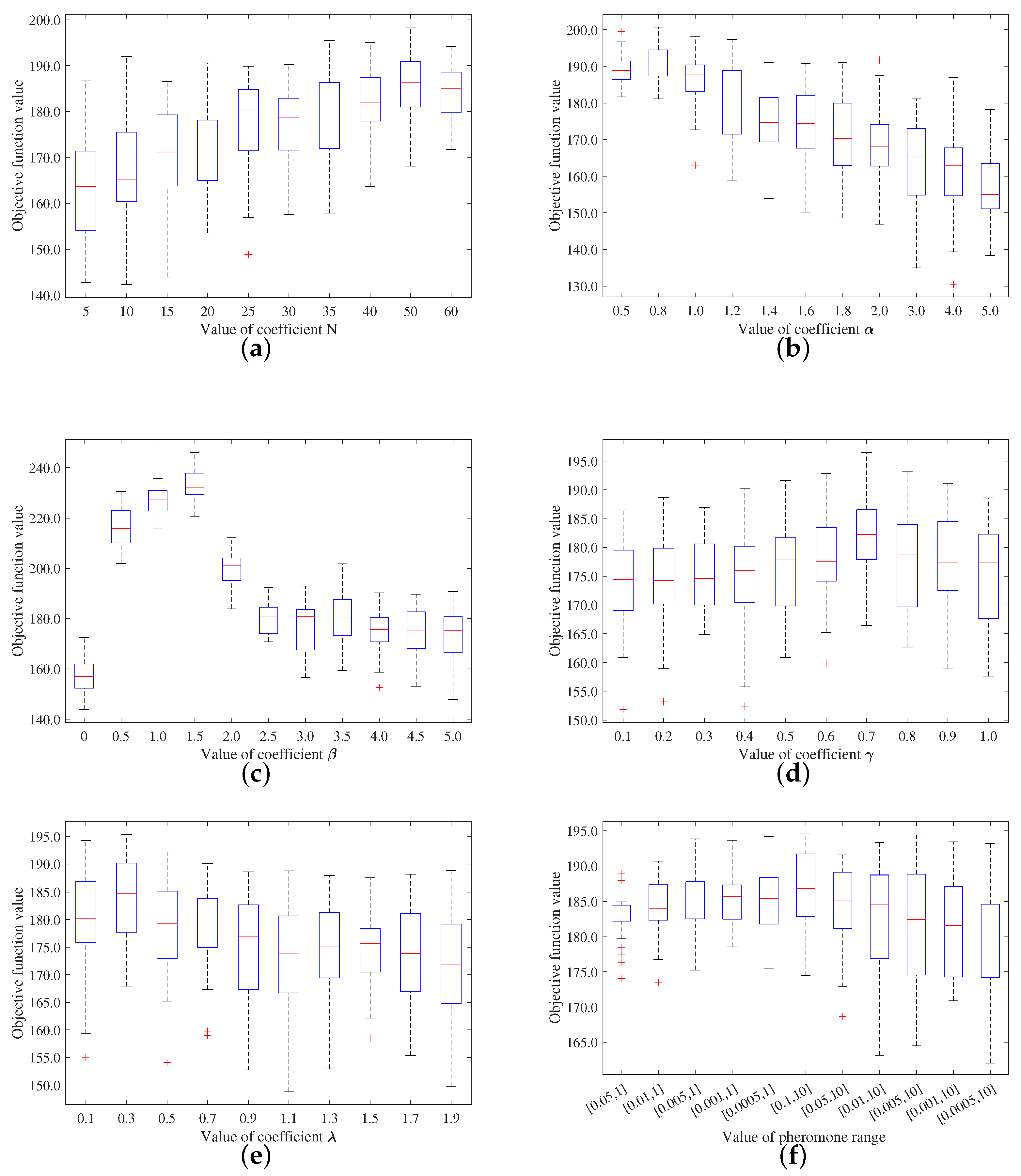
3.2. Analysis of ACO Algorithm Parameter Settings

Given the significance of the number of ants and transition probability in the ACO algorithm, this section explores the impact of the number of ants and the weighting coefficients in Equation (13) on the optimization outcomes. The control variable method is employed to examine the influence of each independent coefficient on the optimal result when one parameter is varied while the others remain constant. We conducted 30 sets of tests and drew box plots. As illustrated in Figure 5, it represents the impact of the number of ants N, the weights $\alpha$, $\beta$, $\gamma$, $\lambda$ of various influencing factors in Equation (13), and the pheromone range on the value of the objective function. The range of values of the parameters of the algorithm is shown in

Table 3. Range of values of the parameters of the algorithm.

Algorithm Parameters	Range of Values
N	$\{5,10,15,20,25,30,35,40,50,60\}$
$\alpha$	$\left\{0.5,0.8,1.0,1.2,1.4,1.6,1.8,2.0,3.0,4.0,5.0\right\}$
$\beta$	$\left\{0,0.5,1.0,1.5,2.0,2.5,3.0,3.5,4.0,4.5,5.0\right\}$
$\gamma$	$\left\{0.1,0.2,0.3,0.4,0.5,0.6,0.7,0.8,0.9,1.0\right\}$
$\lambda$	$\left\{0.1,0.3,0.5,0.7,0.9,1.1,1.3,1.5,1.7,1.9\right\}$
pheromone range	$\begin{array}{c}\left\{\right[0.05,1],[0.01,1],[0.005,1],[0.001,1],\\ [0.0005,1],[0.1,10],[0.05,10],[0.01,10],\\ [0.005,10],[0.001,10],[0.0005,10\left]\right\}\end{array}$

.

Box plots are a statistical visualization tool that provides information about the distribution of data. Each small box in the plot represents five key statistics: the minimum value, the upper quartile, the median, the lower quartile, and the maximum value. These statistics allow us to assess the characteristics of the data distribution. The key features of a box plot include, firstly, the length of the box in a box plot indicates the range in which a large portion of the data is concentrated. A shorter box suggests that the data distribution is less discrete, with less variation between data points. Conversely, a longer box indicates a higher degree of dispersion in the data distribution, implying greater variation between data points. Secondly, the median is represented by a red line within the box plot. It is a measure of central tendency and helps us understand the typical value of the data. When the median is closer to the bottom of the box, it indicates that most of the values are relatively small. Conversely, when the median is located higher up, it suggests that most of the values are larger. Finally, the upper and lower dashed lines, also known as whiskers, extend from the box and represent the variability of the upper and lower quartiles. They reflect the distribution of data points outside the box. Longer whiskers indicate greater variability and larger standard deviations across the data. In this study, the maximum value of the objective function is given priority, followed by the degree of dispersion of the data. With the properties of box plots, it becomes easier to select the optimal set of parameters from Figure 5. Based on this, we can determine that the optimal set of coefficients is $\left[N,\alpha ,\beta ,\gamma ,\lambda \right]=\left[50,0.8,1.5,0.7,0.3\right]$, and the optimal pheromone range is $[0.1,10]$. It is important to highlight that the optimal set of coefficients is closely tied to the specific scenario and will fluctuate with changes in the planning problem.

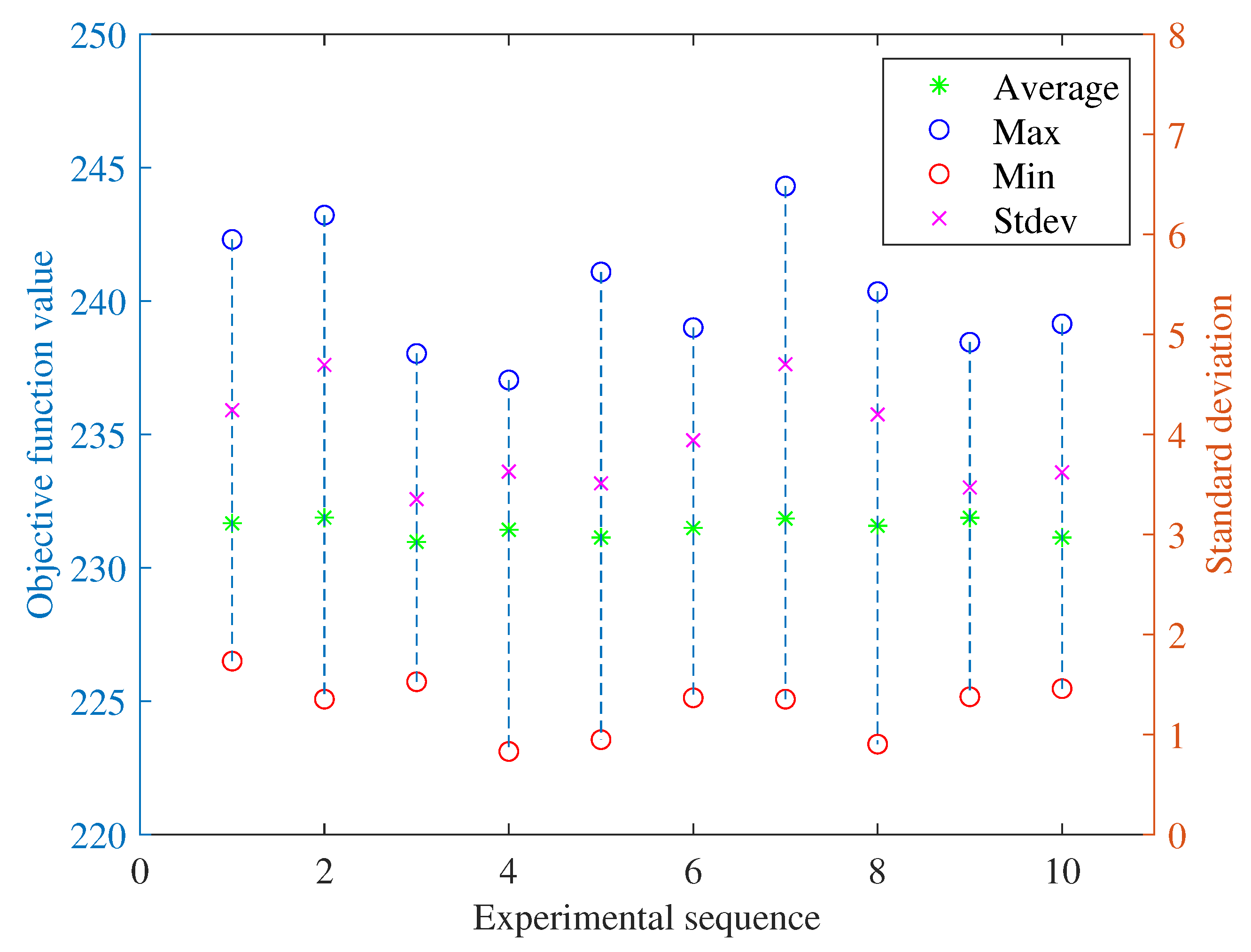
3.3. Algorithm Stability Test

To test the stability of the algorithm, we analyzed the results of calculating the value of the objective function in Equation (11). We conducted ten sets of experiments with 30 runs for each group and calculated the maximum, minimum, mean, and standard deviation for each group. By comparing these statistical metrics, we can assess the stability of the algorithm. As shown in Figure 6, the differences between the maximum, minimum, mean, and standard deviation of the ten groups of experiments are relatively small, indicating minimal variations between different experiments. This demonstrates that the algorithm exhibits good stability within a certain range.

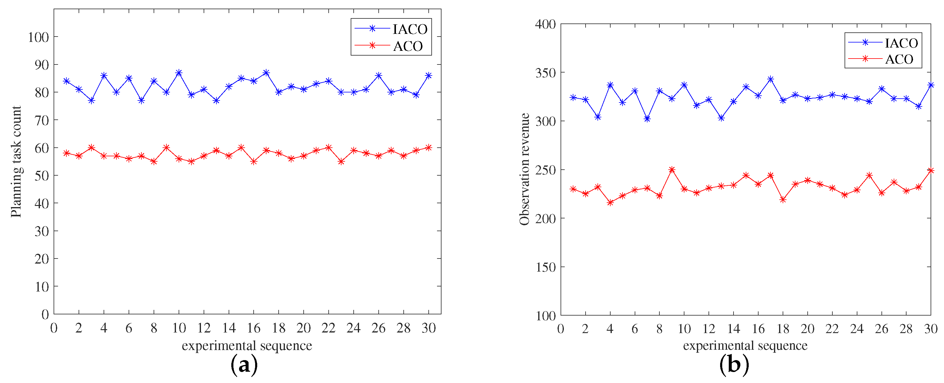
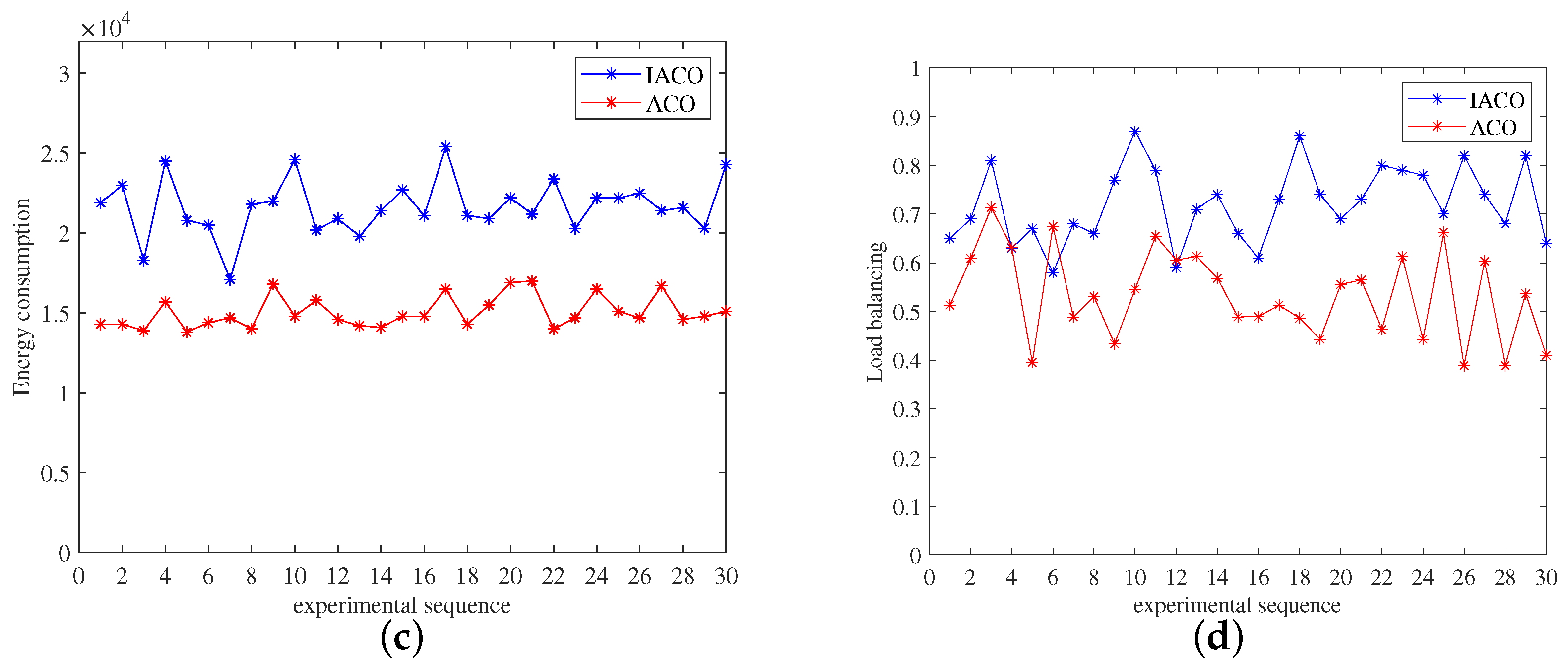
3.4. Simulation Experiment Analysis

This section aims to analyze the planning results of the improved ACO algorithm proposed in the article. Based on the simulation scenario set in Section 3.1, we selected the optimal parameter set analyzed in Section 3.2. The maximum number of iterations was 100 times. The objective function results corresponding to each iteration are shown in Figure 7, which displays the optimal and average objective function values in each iteration. When the number of iterations reached 62, the objective function value reached its peak at 238.219. However, when the number of iterations was 25, the result was 235.627. At this point, the objective function value was only 1.1% different from the optimal objective function value, but it could be achieved 37 iterations earlier. The average objective function value grew rapidly in the first 20 iterations, then slowly in the subsequent 80 iterations, fluctuating around 180. From the above analysis, it can be observed that this algorithm can reach the optimal function value quickly during iterations, and the curve of the average function value also performs well. This demonstrates the effectiveness of the pheromone update strategy and the heuristic factor proposed in this paper.

4. Discussion

With the rapid increase in the number of on-orbit satellites and user demand for dynamic Earth observation, solving the problem of coordinated task planning for multiple agile staring satellites has become the key to meeting user needs and fully utilizing on-orbit satellite resources. To address this issue, this article proposes an improved ACO algorithm for the solution of coordinated mission planning for multiple agile staring satellites. By considering the task interval time, task priority, and the length of time a task can start observation as heuristic information, the improved algorithm has obvious advantages over the traditional ACO algorithm. It can achieve more observation targets and improve observation returns, while also better balancing the load between various satellites, leading to a more reasonable and balanced use of satellite resources.

Figure 8 compares the improved ACO algorithm presented in this paper with the traditional ACO algorithm in terms of the number of planned tasks, observation revenue, energy consumption, and load balancing. Each metric is subjected to 30 sets of comparative experiments to illustrate the superiority of our improved ant colony algorithm over the traditional one.

In this study, we present the improved ACO algorithm, which considers more factors to optimize task planning than the traditional ACO algorithm. The traditional ACO algorithm only considers pheromone concentration and task transfer interval, whereas the improved algorithm adds the priority of the transferred task and the length of time for which observations can be started.

Upon examining Figure 8a in our experiment, it becomes evident that the improved ACO algorithm is capable of observing a greater number of tasks. This is because the changed algorithm takes into account the time interval of the tasks and the length of time for which observations can be started, providing observation opportunities for a larger number of tasks.

As depicted in Figure 8b, the observation gain value achieved by the improved ACO algorithm surpasses that of the traditional ACO algorithm. This superior performance is attributed to the algorithm’s ability to prioritize tasks, enabling high-priority tasks to be observed first. Concurrently, the algorithm’s expansion of the observation time window allows for a greater number of tasks to be observed. This strategic approach not only maximizes task observation but also prevents over-allocation or wastage of resources, thereby ensuring optimal efficiency.

Figure 8c presents a comparative analysis of the energy consumption between the improved ACO algorithm and the traditional ACO algorithm. As the number of planned tasks escalates, there is a corresponding increase in energy consumption. However, the improved algorithm, in a more realistic approach, calculates the minimum energy consumption required for attitude maneuver by taking into account the attitude transfer time. This is a significant improvement over the traditional algorithm, which simplifies energy consumption to a constant value calculation, thereby bringing the improved algorithm closer to practical application scenarios.

Figure 8d illustrates a comparison of the load balancing degree between the improved ACO algorithm and the traditional ACO algorithm. The improved algorithm ingeniously incorporates a load balancing index into the design of the objective function. This inclusion ensures an equitable distribution of tasks among satellites, thereby enhancing the overall system performance and observation efficiency.

In conclusion, the improved ACO algorithm enriches the mission planning process by incorporating heuristic information. This not only facilitates the observation of a greater number of missions but also optimizes the value of observed gains. Furthermore, it significantly improves load balancing and provides a more accurate calculation of attitude maneuver energy consumption. All these advancements contribute to better mission planning and resource management, thereby demonstrating the superiority and practicality of the improved algorithm.

Despite the significant advantages achieved through the improved ACO algorithm presented in this paper, particularly in the realm of collaborative mission planning for multi-agile satellite staring observation, there is still potential for further refinement. In real-world applications, weather fluctuations and cloud cover can greatly influence satellite observations. In practical scenarios, variations in weather and cloud cover can significantly impact satellite observations. Therefore, integrating the influence of factors such as cloud cover into satellite mission planning will be a critical focus of our future research.

5. Conclusions

In conclusion, the goal of this research is to optimize the utilization of on-orbit satellite resources for dynamic monitoring of densely distributed ground point targets. We have proposed an improved ant colony algorithm to solve the mission planning problem for multiple Agile Earth Observation Satellites (AEOSs) in stare observation mode. Our approach utilizes the field of view characteristics of agile stare satellites and applies the DBSCAN clustering algorithm to effectively handle dense point distribution, thereby addressing the challenges posed by observations in dense regions. The results of our experiments validate the effectiveness and feasibility of our approach in mission planning for multiple AEOSs in stare observation mode. By achieving these advances, our research can advance the state of the art in mission planning under satellite staring observation. It provides an effective solution for the rational and comprehensive utilization of satellite resources, enabling efficient monitoring of densely distributed ground point targets. The future track of using this approach involves its integration into operational satellite systems, further refinement based on real-world data, and potential application in other domains requiring resource optimization and target monitoring. Its added value lies in its ability to enhance mission planning efficiency, reduce resource consumption, and to improve the overall effectiveness of satellite-based monitoring systems.

References

1. Chen, X.; Reinelt, G.; Dai, G.; Spitz, A. A mixed integer linear programming model for multi-satellite scheduling. Eur. J. Oper. Res. 2019, 275, 694–707. [Google Scholar] [CrossRef]
2. Hou, A.Y.; Kakar, R.K.; Neeck, S.; Azarbarzin, A.A.; Kummerow, C.D.; Kojima, M.; Oki, R.; Nakamura, K.; Iguchi, T. The Global Precipitation Measurement Mission. Bull. Am. Meteorol. Soc. 2014, 95, 701–722. [Google Scholar] [CrossRef]
3. Dube, T.; Mutanga, O.; Adam, E.; Ismail, R. Intra-and-Inter Species Biomass Prediction in a Plantation Forest: Testing the Utility of High Spatial Resolution Spaceborne Multispectral RapidEye Sensor and Advanced Machine Learning Algorithms. Sensors 2014, 14, 15348–15370. [Google Scholar] [CrossRef]
4. Shakhmatov, E.; Belokonov, I.; Timbai, I.; Ustiugov, E.; Nikitin, A.; Shafran, S. SSAU Project of the nanosatellite SamSat-QB50 for monitoring the Earth’s thermosphere parameters. In Proceedings of the Scientific and Technological Experiments on Automatic Space Vehicles and Small Satellites, Amsterdam, The Netherlands, 31 May 2015; Volume 104, pp. 139–146. [Google Scholar] [CrossRef]
5. Zhang, X.; Wu, M.; Liu, W.; Li, X.; Yu, S.; Lu, C.; Wickert, J. Initial assessment of the COMPASS/BeiDou-3: New-generation navigation signals. J. Geod. 2017, 91, 1225–1240. [Google Scholar] [CrossRef]
6. Zacharias, N.; Dorland, B. The concept of a stare-mode astrometric space mission. Publ. Astron. Soc. Pac. 2006, 118, 1419–1427. [Google Scholar] [CrossRef]
7. Lemaitre, M.; Verfaillie, G.; Jouhaud, F.; Lachiver, J.M.; Bataille, N. Selecting and scheduling observations of agile satellites. Aerosp. Sci. Technol. 2002, 6, 367–381. [Google Scholar] [CrossRef]
8. Habet, D.; Vasquez, M.; Vimont, Y. Bounding the optimum for the problem of scheduling the photographs of an Agile Earth Observing Satellite. Comput. Optim. Appl. 2010, 47, 307–333. [Google Scholar] [CrossRef]
9. Xu, R.; Chen, H.; Liang, X.; Wang, H. Priority-based constructive algorithms for scheduling agile earth observation satellites with total priority maximization. Expert Syst. Appl. 2016, 51, 195–206. [Google Scholar] [CrossRef]
10. Mok, S.H.; Jo, S.; Bang, H.; Leeghim, H. Heuristic-Based Mission Planning for an Agile Earth Observation Satellite. Int. J. Aeronaut. Space Sci. 2019, 20, 781–791. [Google Scholar] [CrossRef]
11. Qiu, W.; Xu, C.; Ren, Z.; Teo, K.L. Scheduling and Planning Framework for Time Delay Integration Imaging by Agile Satellite. IEEE Trans. Aerosp. Electron. Syst. 2022, 58, 189–205. [Google Scholar] [CrossRef]
12. Du, B.; Li, S.; She, Y.; Li, W.; Liao, H.; Wang, H. Area targets observation mission planning of agile satellite considering the drift angle constraint. J. Astron. Telesc. Instrum. Syst. 2018, 4, 047002. [Google Scholar] [CrossRef]
13. Yu, Y.; Hou, Q.; Zhang, J.; Zhang, W. Mission scheduling optimization of multi-optical satellites for multi-aerial targets staring surveillance. J. Frankl. Inst.-Eng. Appl. Math. 2020, 357, 8657–8677. [Google Scholar] [CrossRef]
14. Cui, K.; Xiang, J.; Zhang, Y. Mission planning optimization of video satellite for ground multi-object staring imaging. Adv. Space Res. 2018, 61, 1476–1489. [Google Scholar] [CrossRef]
15. Ji, H.; Huang, D. A mission planning method for multi-satellite wide area observation. Int. J. Adv. Robot. Syst. 2019, 16, 1729881419890715. [Google Scholar] [CrossRef]
16. Vasquez, M.; Hao, J.K. A “logic-constrained” knapsack formulation and a tabu algorithm for the daily photograph scheduling of an earth observation satellite. Comput. Optim. Appl. 2001, 20, 137–157. [Google Scholar] [CrossRef]
17. Xhafa, F.; Herrero, X.; Barolli, A.; Takizawa, M. Using STK Toolkit for Evaluating a GA base Algorithm for Ground Station Scheduling. In Proceedings of the 2013 Seventh International Conference on Complex, Intelligent, and Software Intensive Systems (CISIS), New York, NY, USA, 3–5 July 2013; pp. 265–273. [Google Scholar] [CrossRef]
18. Tangpattanakul, P.; Jozefowiez, N.; Lopez, P. A multi-objective local search heuristic for scheduling Earth observations taken by an agile satellite. Eur. J. Oper. Res. 2015, 245, 542–554. [Google Scholar] [CrossRef]
19. Song, Y.; Ou, J.; Wu, J.; Wu, Y.; Xing, L.; Chen, Y. A cluster-based genetic optimization method for satellite range scheduling system. Swarm Evol. Comput. 2023, 79, 101316. [Google Scholar] [CrossRef]
20. Liu, X.; Laporte, G.; Chen, Y.; He, R. An adaptive large neighborhood search metaheuristic for agile satellite scheduling with time-dependent transition time. Comput. Oper. Res. 2017, 86, 41–53. [Google Scholar] [CrossRef]
21. Long, X.; Wu, S.; Wu, X.; Huang, Y.; Mu, Z. A GA-SA Hybrid Planning Algorithm Combined with Improved Clustering for LEO Observation Satellite Missions. Algorithms 2019, 12, 231. [Google Scholar] [CrossRef]
22. Lu, Z.; Shen, X.; Li, D.; Chen, Y. Integrated Imaging Mission Planning Modeling Method for Multi-Type Targets for Super-Agile Earth Observation Satellite. IEEE J. Sel. Top. Appl. Earth Observ. Remote Sens. 2022, 15, 4156–4169. [Google Scholar] [CrossRef]
23. Bianchessi, N.; Cordeau, J.F.; Desrosiers, J.; Laporte, G.; Raymond, V. A heuristic for the multi-satellite, multi-orbit and multi-user management of Earth observation satellites. Eur. J. Oper. Res. 2007, 177, 750–762. [Google Scholar] [CrossRef]
24. Kebin, G.; Guohua, W.U.; Jianghan, Z. Multi-Satellite Observation Scheduling Based on a Hybrid Ant Colony Optimization. Adv. Mater. Res. 2013, 765–767, 532–536. [Google Scholar] [CrossRef]
25. Song, Y.; Ou, J.; Suganthan, P.N.; Pedrycz, W.; Yang, Q.; Xing, L. Learning Adaptive Genetic Algorithm for Earth Electromagnetic Satellite Scheduling. IEEE Trans. Aerosp. Electron. Syst. 2023, 1–17. [Google Scholar] [CrossRef]
26. Chen, Y.; Xu, M.; Shen, X.; Zhang, G.; Lu, Z.; Xu, J. A Multi-Objective Modeling Method of Multi-Satellite Imaging Task Planning for Large Regional Mapping. Remote Sens. 2020, 12, 344. [Google Scholar] [CrossRef]
27. Liu, Y.; Chen, Q.; Li, C.; Wang, F. Mission planning for Earth observation satellite with competitive learning strategy. Aerosp. Sci. Technol. 2021, 118, 107047. [Google Scholar] [CrossRef]
28. Deng, X.; Dong, Y.; Xie, S. Multi-Granularity Mission Negotiation for a Decentralized Remote Sensing Satellite Cluster. Remote Sens. 2020, 12, 3595. [Google Scholar] [CrossRef]
29. Song, Y.; Wei, L.; Yang, Q.; Wu, J.; Xing, L.; Chen, Y. RL-GA: A Reinforcement Learning-based Genetic Algorithm for Electromagnetic Detection Satellite Scheduling Problem. Swarm Evol. Comput. 2023, 77, 101236. [Google Scholar] [CrossRef]
30. Ou, J.; Xing, L.; Yao, F.; Li, M.; Lv, J.; He, Y.; Song, Y.; Wu, J.; Zhang, G. Deep reinforcement learning method for satellite range scheduling problem. Swarm Evol. Comput. 2023, 77, 101233. [Google Scholar] [CrossRef]
31. He, C.; Dong, Y.; Li, H.; Liew, Y. Reasoning-Based Scheduling Method for Agile Earth Observation Satellite with Multi-Subsystem Coupling. Remote Sens. 2023, 15, 1577. [Google Scholar] [CrossRef]
32. Chen, Y.; Zhou, L.; Bouguila, N.; Wang, C.; Chen, Y.; Du, J. BLOCK-DBSCAN: Fast clustering for large scale data. Pattern Recognit. 2021, 109, 107624. [Google Scholar] [CrossRef]
33. Merkle, D.; Middendorf, M.; Schmeck, H. Ant colony optimization for resource-constrained project scheduling. IEEE Trans. Evol. Comput. 2002, 6, 333–346. [Google Scholar] [CrossRef]
34. Yang, X.S.; Deb, S. Cuckoo Search via Levey Flights. In Proceedings of the 2009 World Congress on Nature & Biologically Inspired Computing (NABIC 2009), New York, NY, USA, 9–11 December 2009; pp. 210–214. [Google Scholar] [CrossRef]
Figure 1. Schematic Representation of Dense Target Point Observation.
Remotesensing 15 05317 g001
Figure 2. Clustering results of target points in dense regions.
Remotesensing 15 05317 g002
Figure 3. Two cases of calculated attitude transfer time.
Remotesensing 15 05317 g003
Figure 4. Mission planning process based on heuristic ACO algorithm.
Remotesensing 15 05317 g004
Figure 5. Effect of different parameters on the results of the objective function. (a) Impact of varying ant numbers N on objective function value. (b) Impact of varying coefficient α on the objective function value. (c) Impact of varying coefficient β on the objective function value. (d) Impact of varying coefficient γ on the objective function value. (e) Impact of varying coefficient λ on the objective function value. (f) Impact of varying pheromone ranges on the objective function value.
Remotesensing 15 05317 g005
Figure 6. Objective function value analysis.
Remotesensing 15 05317 g006
Figure 7. Maximum and average objective values under optimal parameters.
Remotesensing 15 05317 g007
Figure 8. Comparative analysis between improved ACO algorithm and traditional ACO algorithm. (a) Planning task count. (b) Observation revenue. (c) Energy consumption. (d) Load balancing.
Remotesensing 15 05317 g008aRemotesensing 15 05317 g008b