Simulation-Based Self-Supervised Line Extraction for LiDAR Odometry in Urban Road Scenes

Abstract

LiDAR odometry is a fundamental task for high-precision map construction and real-time and accurate localization in autonomous driving. However, point clouds in urban road scenes acquired by vehicle-borne lasers are of large amounts, “near dense and far sparse” density, and contain different dynamic objects, leading to low efficiency and low accuracy of existing LiDAR odometry methods. To address the above issues, a simulation-based self-supervised line extraction in urban road scene is proposed, as a pre-processing for LiDAR odometry to reduce the amount of input and the interference from dynamic objects. A simulated dataset is first constructed according to the characteristics of point clouds in urban road scenes; and then, an EdgeConv-based network, named LO-LineNet, is used for pre-training; finally, a model transferring strategy is adopted to transfer the pre-trained model from a simulated dataset to real-world scenes without ground-truth labels. Experimental results on the KITTI Odometry Dataset and the Apollo SouthBay Dataset indicate that the proposed method can accurately extract reliable lines in urban road scenes in a self-supervised way, and the use of the extracted reliable lines as input for odometry can significantly improve its accuracy and efficiency in urban road scenes.

1. Introduction

As one of the crucial steps of Simultaneous Localization and Mapping (SLAM) technology, odometry, also named registration, estimates relative transformations between consecutive images or point clouds [1], which is vital to cultural heritage protection [2,3], autonomous driving [4,5,6], and mobile robots [7]. However, images captured by visual cameras is easily effected by lighting conditions and weather constraints. Compared with visual cameras, LiDAR can efficiently capture precise 3D geometric details of surroundings within a 360° field of view and can be minimally affected by lighting conditions and weather constraints [8], which is often equipped as an important sensor for odometry tasks [9].

However, urban road scenes are complex and of a wide range, and directly using vehicle-borne laser point clouds for odometry has several challenges: (1) the amount of the original point cloud is large, resulting that directly processing on points being inefficient. To improve the odometry efficiency, researchers attempted to convert point clouds into images, such as LO-Net [10], Delora [7], and EfficientLO-Net [9]. However, these projection-based methods inevitably result in the loss of original 3D information [11]; (2) the density of the original point cloud is “near dense and far sparse”, causing local features of points in two consecutive frames to be inconsistent, making it difficult to find accurate correspondences for point correspondence-based networks, such as DCP [12], DGR [13] and PointDSC [14]. To handle this issue, virtual correspondence-based networks, such as DeepVCP [6], LPD-Net [5], and RegTR [15], have been proposed, however, taking all points into consideration is time consuming, and keypoint-based methods require high repeatability [16]; (3) motions of some dynamic objects, such as vehicles, pedestrians, and tree leaves, are uncertain, and are not consistent with the motion of the vehicle-borne laser [11]. These points should not participate in the relative pose solving, and ought to be filtered out as early as possible in the processing chain. In a word, the above challenges lead to the inability of existing point-based odometry algorithms to meet the requirements of accurate and efficient simultaneous localization and mapping.

Compared with points, lines have obvious advantages in the odometry task. On the one hand, lines can provide position, direction, and length information, with higher descriptiveness, repetitiveness, and robustness [17,18]. PlückerNet [18] represents unordered lines as Plücker coordinates, and PointNet is first employed to learn line-wise features; then, the Sinkhorn solver is used to obtain the correspondencess; finally, the transformation matrix is estimated using the RANSAC algorithm. Experiments on both indoor and outdoor datasets show superiority of efficiency and accuracy. Xu et al. [19] first extracted lines by the method of Lu et al. [20] and classified them into three types according to their direction, and then constructed 2-line congruent sets (2LCS) with the RANSAC algorithm to achieve optimal transformation. It is more robust, with repetitive components, symmetrical structures, and limited overlap. On the other hand, for LiDAR odometry in urban road scenes, by extracting lines, dynamic objects, such as vehicles and pedestrians, even tree leaves, can be effectively filtered, avoiding their participation in the relative pose solving. In addition, the use of lines as input for odometry can effectively decrease the amount of input, consequently enhancing efficiency. However, existing traditional line extraction methods are not specific to certain line types, and tend to mistakenly extract the virtual lines caused by scanning lines; thus, they are not suitable to extract reliable lines defined in urban road scenes. Moreover, there is currently no labeled dataset of line extraction in urban road scenes for deep learning-based methods. Although we can utilize the existing semantic segmentation dataset to construct a line classification dataset, obtaining high-resolution intersection lines of building planes in semantic segmentation results requires a very fine level of granularity. Superline3D [21] pioneered a line extraction method based on a small synthetic dataset, which can effectively extract lines without the need for real annotated datasets.

To address the above issues, inspired by Superline3D [21], this paper proposes a simulation-based self-supervised line extraction for LiDAR odometry in urban road scenes. As shown in Figure 1, considering that there is no labeled dataset and the manual labeling is time-consuming, a simulated dataset with ground-truth labels is first constructed based on the characteristics of vehicle-borne laser point clouds in urban road scenes; secondly, local scale-invariant features are computed to eliminate the scale factor between the simulated dataset and the real scene, and a proposed LO-LineNet is trained on the simulated dataset with local scale-invariant features for pre-training; finally, a model transferring strategy is adopted to transfer the model from the simulated dataset to the real scenes to obtain accurate labels, with a RANSAC-based line fitting to filter noise. Our contributions are summarized below:

(1)

a heuristic simulated dataset construction strategy is proposed, with characteristics that are very similar to those of the real scenes;

(2)

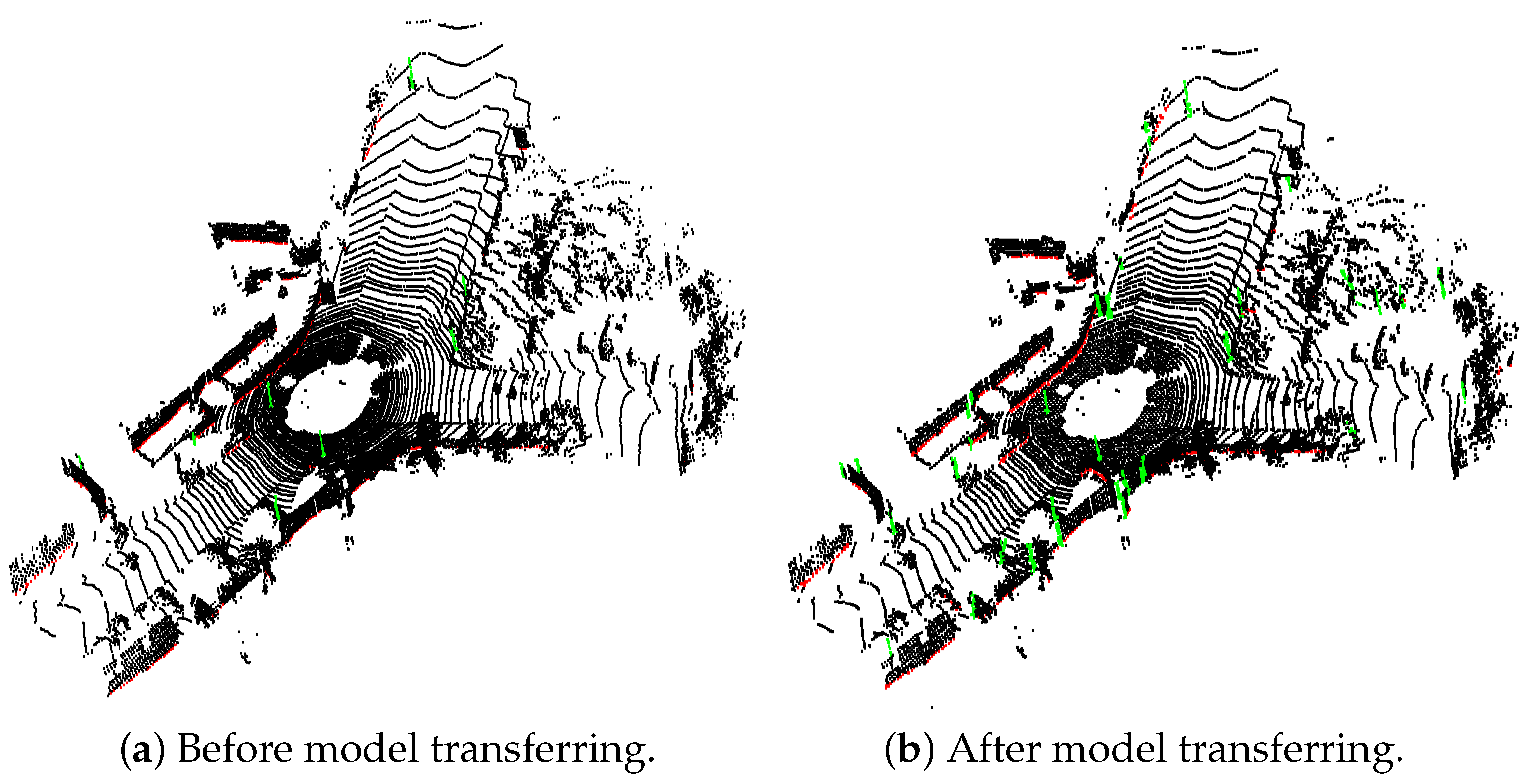
a model transferring strategy is adopted to transfer the model from the simulated dataset to real scans;

(3)

experiments on the KITTI Odometry Dataset and the Apollo SouthBay show that this method can effectively extract reliable lines in road scenes by model transferring on few simulated data;

(4)

experiments show that using the extracted lines as input for LiDAR odometry in urban road scenes can greatly improve its accuracy and efficiency, especially cimbined with deep learning-based networks.

2. Related Works

2.1. LiDAR Odometry

Due to the mentioned challenges of vehicle-borne laser point clouds in urban road scenes, traditional local feature descriptor-based methods and ICP-based [22] methods often perform poorly in both accuracy and efficiency. Recently, deep learning-based odometry networks have demonstrated promising performance on publicly available datasets. These networks can be classified into two distinct categories: 2D projection-based pose regression networks and point correspondence-based networks. The former inevitably loses the original 3D information [11]. The following mainly introduces point correspondence-based networks.

Lu et al. [6] proposed the first virtual correspondences-based registration network named DeepVCP. It used PointNet++ [23] to learn pointwise local features, selected keypoints through a point weighting layer, and finally generated virtual correspondences through a point generation layer. Similarly, Wei et al. [5] proposed a registration network named LPD-Registration. It enhanced structural information and correlation information through self-attention and cross-attention mechanisms, and generated K best correspondences through a virtual corresponding point generation module. These virtual correspondence-based methods directly estimate the virtual correspondences of keypoints without eliminating incorrect correspondences, achieving comparable registration accuracy and efficiency. DGR [13] first used FCGF [24] to learn pointwise features, and then evaluated confidences of matching relationships using a 6D convolutional neural network, finally estimating the pose parameters using a differentiable weighted Procrustes algorithm [25]. It is of high accuracy and strong adaptability. PREDATOR [26] can detect inliers/outliers of two point clouds and solve the relative transformation simultaneously. This method can still achieve high registration accuracy in low-overlap scenarios. To deal with the situations with insufficient overlap, or the presence of dynamic objects, Fischer et al. [27] proposed a network that operates directly on sparse keypoints. First, the keypoints are subject to different levels of feature extraction through a Pillar Encoder and a Positional Encoder. Then, multiple multi-head self-attention and cross-attention modules are used to integrate contextual information. Finally, a refinement transfer layer is employed to obtain the keypoint matching relationships. This method exhibits strong robustness even in high-speed scenes and when frames are lost. GeoTransformer [28] codes pair-wise distances and triplet-wise angles to learn geometric feature for robust superpoint matching, making it robust in low-overlap cases and invariant to rigid transformation. Wang et al. [1] proposed an oriented descriptors and local rotations-based registration framework. By incorporating the two elements into the entire registration process, it significantly improved the registration reliability and efficiency. To address the challenges posed by the significant dimensional differences, semantic gaps, and mutual interference caused by mixed features, Wang et al. [29] proposed a registration network called MFGNet that utilizes spatial coordinates and local features to guide the search for matching points. Unlike methods that directly use mixed features, MFGNet consists of two different matching matrix computations: coordinate matching matrix computation and feature matching matrix computation. These two branches independently learn to assign correct correspondences, and then their respective matching matrices are fused to obtain the final matching matrix. The rigid transformation parameters are subsequently solved using a differentiable SVD algorithm. This network achieves high registration accuracy while maintaining computational efficiency.

In general, point correspondence-based networks are robust to initial positions and can achieve high precision when the data quality is good. However, they mostly use points as the basic unit, which is of a large amount, and do not consider the interference of dynamic objects in urban road scenes, leading to low efficiency and accuracy.

2.2. Line Extraction

Current line extraction methods from point clouds can be mainly categorized into two types: (1) converting point clouds into images [20,30]; (2) analyzing the geometric or radiative features of point clouds to extract lines [31], such as curvature, normal and intensity. The following text introduces the two types.

Projection-Based Methods: Zhu and Hyyppä [30] used statistical analysis based on geometric information to extract power lines; the analysis is automated and computationally effective. Wang et al. [31] and Zhou et al. [32] first projected the point clouds of power transmission into 2D images, and then, 2D Hough transformation was used to extract power lines. This method can ensure the continuity of line segments to some extent. Lu et al. [20] proposed a fast line extraction method based on planes. Normal-based segmentation was first adopted to initially obtain the planes, and region growing was used to refine extracted planes; then, a 3D–2D projection was applied to ectract lines on 2D binary images via Least Square Fitting; finally, a 2D–3D projection was used to obtain the corresponding 3D line segments. However, these projection-based methods highly relied on projection transformation [33], inevitably leading to the missing of the lines that are perpendicular to the projection.

3D Line Extraction Methods: Fang et al. [34] separated road markings from road surface by an intensity-based k-means clustering, and then refined the results by normalized cuts with geometric features and spatial distributions. However, this method cannot handle partial solid line misextraction and missed extraction due to sparse density. Zhang et al. [35] came up with a multi-conditional GAN to extracted contours for outdoor scenes. Specifically, a parametric space-based framework and a guided learning framework were, respectively, used to reduce the point space and acquire the target distribution. However, this required a labeled dataset, and it was not end-to-end. Hu et al. [36] proposed a geometric feature enhanced line extraction method. Planes were first extracted by normal and curvature-based region growing and merging, and then line candidates were extracted by a 3D–2D projection, pretrained DexiNed [37] and MCMLSD [38] algorithm; finally, candidate lines were optimized by the hierarchical topology between contours and lines. It can filter out major miscellaneous and broken lines. Liu et al. [17] proposed a supervoxel segmentation based on Euclidean distance and normal vectors to extract feature lines. This method can simultaneously extract lines of three types with high accuracy. Zhao et al. [21] proposed the first self-supervised line segmentation named Superline3D. A synthetic dataset was first generated, and then a geometric adaptation strategy was adopted for automatic line labeling. However, the generated simulated dataset was significantly different from the real road scene dataset, and iterations were required for high accuracy. Jiang et al. [33] came up with a general 3D structural line extraction method from point clouds with a single building as input. Corner points were first extracted by an associative learning module, and then a graph neural network (GNN) was adopted to learn the curve connections. Experiments on outdoor building, indoor scene, and furniture point clouds verified the strength and efficacy. However, semantic segmentation is required to obtain instance-level buildings from raw point clouds.

To sum up, existing traditional line extraction methods can achieve high accuracy in some specific scenarios according to the geometric or radiative features. However, that makes it difficult to manually tune parameters for the complicated large-scale point clouds, and lines in specific types cannot be selectively detected. Moreover, for deep learning-based methods, there is no labeled dataset, and manual labeling is time-consuming.

3. Methodology

3.1. Simulated Dataset Construction

Generally speaking, lines in urban road scenes acquired by vehicle-borne laser can be divided into three categories [21]: (1) standalone pole objects, such as street lamps; (2) intersections of planes, such as intersections between buildings and the ground, and intersections between different faces of buildings; (3) virtual lines, formed by edge points across the scanning rings. Among them, lines of the first two types are relatively reliable in LiDAR odometry, so this paper aims to extract lines of the two types, which are defined as reliable lines.

In order to simulate these three types of lines in urban road scenes, as shown in Figure 2, four graphic primitives are used: (1) multiple circular rings to simulate the ground; (2) a vertical line to simulate a standalone pole object; (3) a plane to simulate a building facade; and (4) two perpendicular planes to simulate two perpendicular building facades. Then, since lines in different types are of different features, we label reliable lines into two categories: simulated independent pole objects are labeled as Category 1 (colored in green), simulated intersections between planes are labeled as Category 2 (colored in red), and the rests are labeled as Category 0 (colored in black).

To make the point cloud of the simulated ground closer to the real road scenes, each circular ring of the simulated ground is uniformly sampled with a fixed number, with the distance between each circular ring gradually increasing from inside to outside, so that the density is “near dense and far sparse”. Then, the point cloud of the simulated ground is clipped, and only points with an absolute value of the y coordinate less than 3 m are retained, forming a simulated road. As for the other three graphic primitives, they are first uniformly sampled according to a fixed density to generate simulated point clouds. To simulate the incomplete objects caused by occlusion in real scenes, 10% of the points are clipped for the three graphic primitives. Finally, the processed point clouds of three graphic primitives are placed on both sides of the simulated road.

Considering the noise in the real point cloud, all simulated points are effected by Gaussian noise with a mean of zero and a standard deviation of 0.01 mr on each axis. In addition, as shown in Figure 3, a portion of vegetation and vehicles from real scanning data, totaling 2000 points, are randomly cropped and combined to form the final simulated data. The final simulated dataset includes 1300 point clouds, 1000 for training and 300 for testing, with an approximate count of 13,000 points per point cloud.

3.2. Scale-Invariant Feature Computation

The main challenge of this method is the scale difference between real LiDAR point clouds and the simulated dataset. Similar to Superline3D [21], a scale-invariance feature $f_i$ is computed:

$$f_i=\frac{p-p_i}{∥p-p_i∥},i=1,2,\dots ,k.$$

(1)

In Equation (1), k nearest points $\left\{p_1,p_2,\dots ,p_k\right\}$ of point p are searched, and the scale-invariant local feature $f_i$ is calculated as a unit vector between p and its neighboring point $p_i$.

3.3. Network Architecture

We consider the reliable line extraction as a classification problem, and propose a network named LO-LineNet. As shown in Figure 4, the input of LO-LineNet is point clouds with scale-invariant features, and the LO-LineNet is composed of two modules: a feature encoder and a classification decoder.

Feature Encoder: in the first module, two EdgeConv [39] layers are first adopted to extract features of the k-nearest neighbors for each point. The EdgeConv is proficient in capturing neighborhood features, and we use the coordinate of point clouds as the nodes of the graph, and the scale-invariant features are as edges; then, two multi-head self-attention [40] layers are applied for information communication between their neighborhoods, so that attention can be focused on important points in their neighborhoods, reducing the effect of redundant points; finally, the original neighborhood features and self-attention features are aggregated and input into the third EdgeConv [39] layers to obtain pointwise local features sized N × 1024 (N is the amount of points) after a Maxpool layer.

Classification Decoder: in the decoder module, three basic convolution layers are adopted to compress the obtained feature vectors sized N × 1024 to a tensor sized N × 3. And then, through a Softmax layer, the probability of each point belonging to three categories is obtained (the sum of the probabilities of the three categories is 1). Finally, an Argmax layer is applied, the index with the highest probability are regarded as the category of the point. We use ReLU for activation, InstanceNorm for normalization.

3.4. Loss Function

The loss function L is a standard cross-entropy loss, expressed as follows:

$$L=-{\sum }_{i=0}^{c-1}{y}_{i}log\left(p_i\right),$$

(2)

where $p=[p_0,p_1,\dots ,p_{c-1}]$ is a probability distribution, and $p_i$ denotes the probability associated with the point belonging to the ith class; $y=[y_0,y_1,\dots ,y_{c-1}]$ is a one-hot encoding representation of the point label, and if the point belongs to the ith category, $y_i$ = 1; otherwise, $y_i$ = 0. c is the number of labels.

3.5. Model Transferring

Although the constructed simulated dataset has a huge gap compared with the complicated real road scenes, the features of lines in the two scenes have certain commonalities. Thus, a model transferring strategy is used to transfer the model from the simulated dataset to the real scenes.

As shown in Figure 1, the model transferring process includes three flows: pre-training flow, test flow and fine-tuning flow.

Pre-training Flow: for the predefined simulated dataset, scale-invariant features are first computed, and then, point clouds with scale-invariant features are input into the LO-LineNet to pre-train a scale-invariant classification model;

Test Flow: scale-invariant features of the real-world dataset are first computed, and then the real-world dataset with scale-invariant features are input into the the LO-LineNet trained on simulated dataset to directly predict the labels of the real-world dataset. Since LO-LineNet predicts the label of each point, labels may be discrete and misclassified. Finally, a distance and normal-based region growing algorithm and a RANSAC-based line fitting algorithm are used to filter discrete and misclassified labels (as shown in Figure 5). The point cloud of the remaining labels of each cluster is regarded as reliable lines.

Fine-tuning Flow: in this flow, the reliable lines of real-world dataset obtained from the test flow are taken as the groundtruth, and then the pre-trained Lo-LineNet is retrained on real-world dataset guided by groundtruth, which is named a fine-tuning flow. After that, a model suitable for real-world scenarios is obtained. It is worth noting that we only adopt the fine tuning one time to automatically generate labels with high accuracy.

4. LiDAR Odometry

The method aims to extract reliable lines in urban road scenes for accurate and efficient LiDAR odometry, as it can reduce the amount of points and the interference of dynamic objects. Most notably, our method can finally output two representations of reliable lines: one is the original reliable lines represented as points, and the other is the fitted line segments represented as vectors; we only use the first representations in the following experiments, as the existing odometry methods or networks, such as ICP [22], GICP [41], GeoTransformer [28] and RegTR [15], only support input in the form of points.

The diagram of using extracted reliable lines as input for LiDAR odometry is shown in Figure 6. The original point clouds of the source and the target are first preprocessed by our LO-LineNet to extract reliable lines in urban road scenes; then, odometry methods or networks are applied to obtain the relative pose between the source and the target; finally, the sources are aligned to the target with the relative pose.

5. Dataset, Experimental Setting, and Metrics

Dataset: the KITTI Odometry Dataset [42] and the Apollo SouthBay Dataset [43] are used for experiments, which are acquired by vehicles driven at varying speeds (from 30 km/h to 100 km/h) in varying environments (highway, urban, country, and the combaination of urban and country). It is noteworthy that the driving distances of the Apollo SouthBay Dataset are much longer than those of the KITTI Odometry Dataset. Details of the two datasets are listed in

Table 1. Details of the KITTI Odometry Dataset.

Sequence	00	01	02	03	04	05	06	07	08	09	10
Distances	3714	4268	5075	563	397	2223	1239	695	3225	1717	919
Frame	4541	1101	4661	801	271	2761	1101	1101	4071	1591	1201
Max speed	46	96	49	31	56	48	51	39	43	52	51
Environment	Urban	Highway	Mixed	Country	Country	Urban	Urban	Urban	Mixed	Mixed	Mixed

“Frame” means the the number of point cloud frames in each sequence. “Mixed” means a combination of urban and country. The unit of “Distance” and “Max speed” are, respectively, meter and kilometer/hour.

and

Table 2. Details of the Apollo SouthBay Dataset.

Route	Baylands to Seafood		Mathilda AVE		Columbia Park		San Jose Downtown			Highway 237
Sequence	00	01	02	03	04	05	06	07	08	09	10
Distance	4435	6254	9990	9741	8825	14,675	3420	6285	3204	9695	12,175
Frame	6443	7538	10,903	11,846	14,014	20,801	9765	16,596	9868	4701	5677
Max speed	74	68	67	74	44	48	37	45	37	105	100
Environment	Highway	Highway	Highway	Highway	Urban	Urban	Urban	Urban	Urban	Highway	Highway

“Frame” means the the number of point cloud frames in each sequence. The unit of “Distance” and “Max speed” are, respectively, meter and kilometer/hour.

, respectively.

Experimental Setting: for model pre-training, LO-LineNet is initially trained on the simulated dataset for 50 epochs; then, the pre-trained LO-LineNet is trained on the KITTI Odometry Dataset for other 50 epochs for model finetuning. Sequences 00–05 in the KITTI Odometry Dataset are used for training, and sequences 06–07 are used for validation. Each point cloud is sampled with a 0.3 m voxel size, with approximately 20,000 points. All sequences of the Apollo SouthBay Dataset are used for testing to verify the generalization of the proposed method.

Training Details: the whole network is implemented in pytorch with an Adam optimizer. For both model pre-training and model transferring processes, the initial learning rate is configured as 0.001 and decreased by 50% every 10 epochs. The batchsize of the pre-training process it set to four, and the batchsize of model transferring process is set to onr. The whole network is trained on a NVIDIA TITAN RTX GPU.

6. Experimental Results

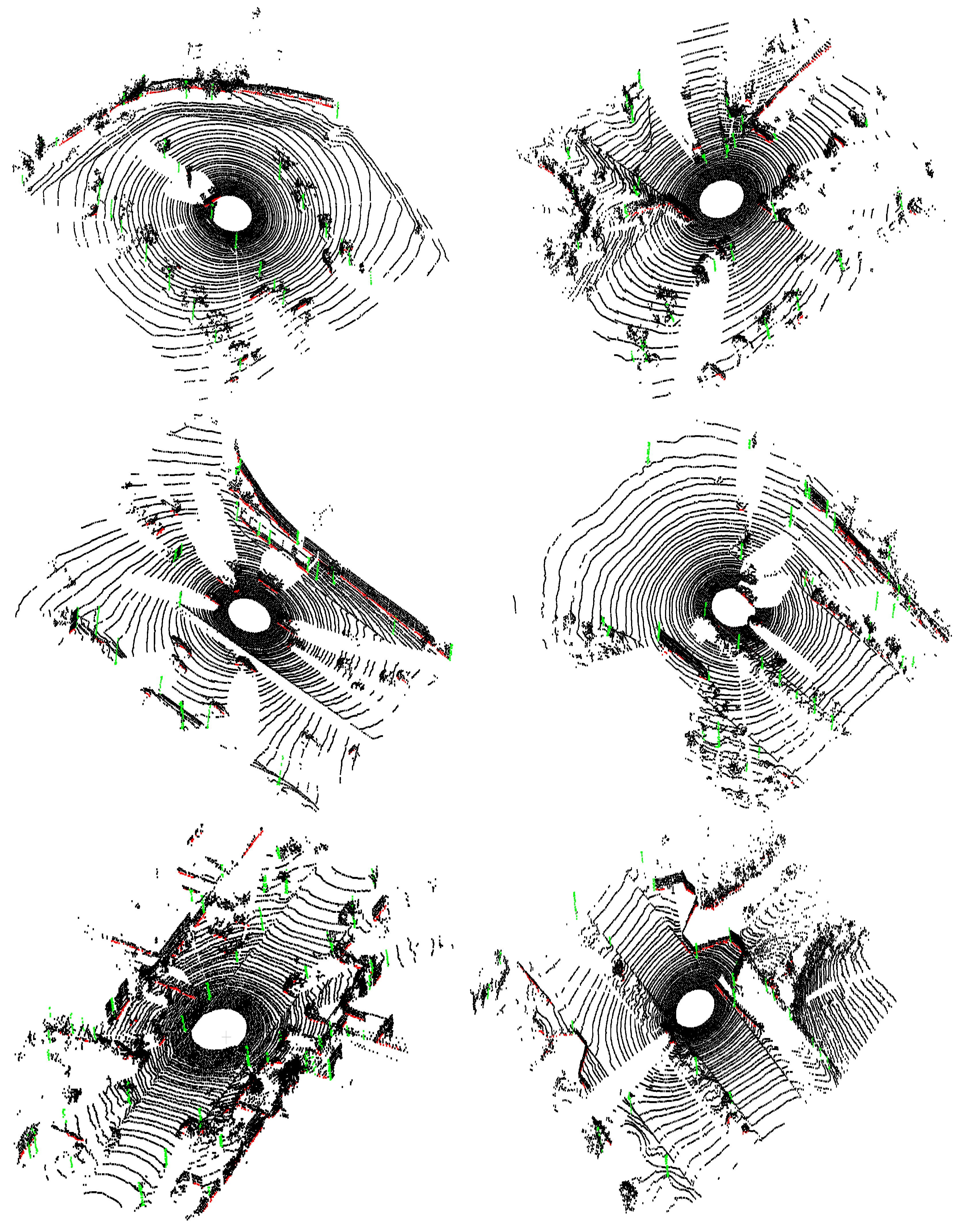
6.1. Results of Reliable Line Extraction

For a real dataset, as it lacks ground truth of reliable lines, only qualitative evaluations are conducted in this section. To facilitate a visual comparison, randomly selected results in the KITTI Odometry dataset of 3dLineDetection [20], Superline3D [21] and our LO-LineNet are presented in Figure 7. Results of dLineDetection [20] and Superline3D [21] are obtained by the execution of the authors’ published codes.

From Figure 7, it is obvious that (1) 3dLineDetection missed all pole-like objects. This is because 3dLineDetection is a projection-based method. Pole-like objects are perpendicular to the projection direction. After vertical projection, pole-like objects become a point on a projection plane. Additionally, 3dLineDetection tended to detect virtual lines formed by the scanning rings as reliable lines. This is because after projection, the scan lines approximate straight lines at the edge of the scenes; (2) Superline3D [21] mistakenly detects the points near intersections as well, especially the intersection of planes, resulting in extracted lines having a certain width. This is due to the fact that it categorizes the intersection of planes and rod-shaped objects as one type to extraction. The pole-like object has a certain width and the network learns this feature through training, leading to the detection of nearby points when detecting plane intersections. After iteration, the extracted plane intersection lines become wider and wider. On the other hand, it often suffers from more severe detection deficiencies, especially when it comes to standalone pole objects in the edge of the scene. This is due to the fact that during the model transferring process, the learned features are lines with a certain width, while the density of pole-like objects at the scene edges is relatively sparse, resulting in missing data; (3) our LO-LineNet can accurately extract intersection of planes and mostly all pole-like objects in the scene, owing to the novel simulation strategy considering common line categories in real scenes and dividing them into different categories based on their characteristics and the model transferring strategy.

6.2. Effect of Model Transferring

Model transferring is the core component of the method, supposed to transfer the model from the simulated dataset to real scenes, as the features of lines in the two scenes have certain commonalities. To verify the feasibility of this strategy transferring from a small simulated dataset to complicated real scenes, we record reliable line extraction results before model transferring and after model transferring.

As shown in Figure 8, direct usage of the model learned from the simulated dataset to predict the real dataset can only extract some lines whose characteristics are very similar to those of the simulated data, especially pole-like objects. This is because the standalone pole-like objects defined in the simulation dataset are too idealized, simulated by only a straight line perpendicular to the ground. When it comes to tree trunks with some noise around or streetlights in the scene edge, the extraction often fails without transferring. However, after model transferring, more standalone pole-like objects, such as streetlights, billboards, especially tree trunks, are detected. This is because, through model transferring, the features learned on the simulated dataset are fine tuned to better align with the characteristics of the real scenes, which shows the feasibillity of the strategy of transferring the model from a small simulated dataset to real scenes.

6.3. Generalization on Unseen Dataset

To test the generalization of the proposed method on the unseen dataset, we use the model transferred on the KITTI Odometry Dataset to directly predict the labels of the Apollo SouthBay Dataset without any fine-tuning. Similar to the pre-processing of the KITTI Odometry Dataset, each point cloud in the Apollo SouthBay Dataset is down-sampled with a 0.3 m voxel size, with approximately 20,000 points. It worth noting that all sequences of the Apollo SouthBay Dataset are used for testing to verify the generalization of the proposed method.

Figure 9 depicts the reliable line extraction results of the Apollo SouthBay Dataset. It worth noting that the Apollo SouthBay Dataset is more complex, and there are more pole-like objects icompared to the KITTI Odometry Dataset, and the intersectioin of planes is quite different from that of the KITTI Odometry Dataset in the training process. This brings a big challenge for our methods. However, it is obvious in Figure 9 that reliable lines in the Apollo SouthBay Dataset, regardless of whether the intersections are of planes or pole-like objects, still can be accurately extracted without any model finetuning. This is owing to the model transferring strategy. Through model transferring, the common characteristics of reliable lines between the simulated dataset and the real datasets are strengthened, such as the intersections of planes and independent features of pole-like objects. Although the Apollo SouthBay Dataset and the KITTI Odometry Dataset are different, the characteristics of the reliable lines in the two datasets are very similar. In addition, the scale-invariant features can eliminate the influence of inconsistent scales between the two datasets. Thus, good performances on the Apollo SouthBay Dataset can be obtained, which shows our method has good generalization.

6.4. Accuracy of LiDAR Odometry

Since only qualitative evaluations are conducted on reliable line extraction, in this section, we indirectly reflect the quality of line extraction results by evaluating the accuracy of LiDAR odometery using our LO-LineNet as a preprocessing to assess the feasibility and superiority of our LO-LineNet for subsequent LiDAR odometry. A series of experiments are conducted on the KITTI Odometry Dataset and the Apollo SouthBay Dataset. Official metrics $t_{rel}$, $r_{rel}$ computed by the odometer evaluation toolkit officially provided by KITTI [42] are adopted to evaluate the accuracy of rotation and translation in LiDAR odometry. Traditional methods like ICP [22], GICP [41] and LOAM [44], and deep learning-based methods like GeoTransformer [28] and RegTR [15] are used for comparison.

6.4.1. Accuracy of the KITTI Odometry Dataset

Table 3. The LiDAR odometry accuracy on the KITTI Odometry Dataset.

Method	Metrics	00	01	02	03	04	05	06	07	08	09	10	Average
Full LOAM [44]	$t_{rel}$	0.78	1.43	0.92	0.86	0.71	0.57	0.65	0.63	1.12	0.77	0.79	0.84
	$r_{rel}$	0.53	0.55	0.55	0.65	0.50	0.38	0.39	0.50	0.44	0.48	0.57	0.50
Full A-LOAM	$t_{rel}$	0.76	1.97	4.53	0.93	0.62	0.48	0.61	0.43	1.06	0.73	1.02	1.19
	$r_{rel}$	0.31	0.50	1.45	0.49	0.39	0.25	0.28	0.26	0.32	0.31	0.40	0.45
A-LOAM ${}^{†}$	$t_{rel}$	4.08	3.31	7.33	4.31	1.60	4.09	1.03	2.89	4.82	5.76	3.61	3.89
	$r_{rel}$	1.69	0.92	2.51	2.11	1.13	1.68	0.52	1.80	2.08	1.85	1.76	1.64
CLS [45]	$t_{rel}$	2.11	4.22	2.29	1.63	1.59	1.98	0.92	1.04	2.14	1.95	3.46	2.12
	$r_{rel}$	0.95	1.05	0.86	1.09	0.71	0.92	0.46	0.73	1.05	0.92	1.28	0.91
Velas et al. [46]	$t_{rel}$	3.02	4.44	3.42	4.94	1.77	2.35	1.88	1.77	2.89	4.94	3.27	3.15
	$r_{rel}$	NA	NA	NA	NA	NA	NA	NA	NA	NA	NA	NA	NA
LO-Net [6]	$t_{rel}$	1.47	1.36	1.52	1.03	0.51	1.04	0.71	1.70	2.12	1.37	1.80	1.33
	$r_{rel}$	0.72	0.47	0.71	0.66	0.65	0.69	0.50	0.89	0.77	0.58	0.93	0.69
ICP-po2pl [47]	$t_{rel}$	3.80	13.53	9.00	2.72	2.96	2.29	1.77	1.55	4.42	3.95	6.13	4.74
	$r_{rel}$	1.73	2.58	2.74	1.63	2.58	1.08	1.00	1.42	2.14	1.71	2.60	1.93
ICP-po2po [22]	$t_{rel}$	6.88	11.21	8.21	11.07	6.64	3.97	1.95	5.17	10.04	6.92	8.91	7.36
	$r_{rel}$	2.99	2.58	3.39	5.05	4.02	1.93	1.59	3.35	4.93	2.89	4.74	3.41
ICP-po2po * [22]	$t_{rel}$	6.27	31.16	8.83	4.73	7.28	3.98	5.44	5.09	9.31	6.32	8.38	8.80
	$r_{rel}$	2.76	3.18	3.15	4.26	4.88	1.83	1.97	2.27	3.07	2.30	3.64	3.03
GICP [41]	$t_{rel}$	1.29	4.39	2.53	1.68	3.76	1.02	0.92	0.64	1.58	1.97	1.31	1.92
	$r_{rel}$	0.64	0.91	0.77	1.08	1.07	0.54	0.46	0.45	0.75	0.77	0.62	0.73
GICP * [41]	$t_{rel}$	2.96	19.77	3.59	2.80	3.59	2.23	2.31	1.82	3.33	4.25	2.88	4.50
	$r_{rel}$	1.61	2.16	2.07	1.86	2.07	0.92	1.32	1.24	1.46	1.52	1.89	1.65
GeoTransformer [28]	$t_{rel}$	2.20	3.23	7.42	4.99	3.30	2.11	3.00	2.52	2.52	3.58	3.29	3.47
	$r_{rel}$	0.80	0.90	1.62	1.46	0.48	0.88	1.21	2.32	0.96	1.24	1.39	1.21
GeoTransformer * [28]	$t_{rel}$	2.55	2.85	2.99	1.96	1.58	2.71	1.16	2.15	3.94	5.74	4.18	2.89
	$r_{rel}$	1.42	2.29	1.26	0.98	0.94	1.46	0.71	1.40	1.83	5.23	1.77	1.76
RegTR [15]	$t_{rel}$	2.23	5.03	3.19	1.92	2.40	3.24	1.51	11.33	5.13	7.42	5.55	4.45
	$r_{rel}$	1.10	1.40	1.21	0.82	0.88	1.42	0.79	2.06	3.78	3.00	2.93	1.76
RegTR * [15]	$t_{rel}$	1.46	2.29	1.55	1.31	0.48	0.99	1.03	1.13	2.04	2.36	1.86	1.50
	$r_{rel}$	0.77	0.61	0.65	0.73	0.39	0.51	0.50	0.95	0.94	0.92	0.88	0.71

“†” means method without mapping, “*” means using extracted lines as input. ICP-po2po * [22] and GICP * [41] are executed through open3d. Results of GeoTransformer [28] and RegTR [15] were obtained by the execution of the authors’ published code. Other results are cited from [9]. Best results displayed in bold.

lists the odometry accuracy of typical traditional methods and deep learning networks in the KITTI Odometry Dataset. It is noteworthy that for the deep learning methods, we use sequences 00–06 in the KITTI Odometry Dataset as training sets and sequences 07–10 as testing sets.

It is obvious that, for ICP [22] and GeoTransformer [28], using extracted reliable lines as input for LiDAR odometry can significantly improve accuracy in some sequences, while for RegTR [15], using extracted lines as input achieves higher accuracy in all sequences compared to using all points as input. This is because RegTR [15] is a virtual correspondence-based network, which can handle the problem of correspondences in two consecutive frames to be inconsistent due to irregular point cloud density, while ICP [22] and GeoTransformer [28] both highly rely on the accurate correspondences. It noteworthy that in Sequence 04, RegTR [15] with extracted reliable lines as input, achieves the highest accuracy in both rotation and translation, even compared to Full LOAM [44] and Full A-LOAM, showing the superiority of virtual correspondence-based network with the extracted reliable lines as input. However, for GICP * [41], using reliable lines as input did not improve the accuracy of the odometery; it decreased in most sequences because of the global optimization. Furthermore, for traditional methods, like ICP * [22] and GICP * [41], using reliable lines as odometry input results in poor performances in highway scenes, as there are few reliable lines after extraction, such as Sequence 01. Surprisingly, for deep learning-based methods, like GeoTransformer * [28] and RegTR * [15], using reliable lines as odometry input still results in higher accuracy in Sequence 01 such as with highway scenes than when using all points as input, which demonstrates an enormous potential of deep learning-based methods.

6.4.2. Accuracy of the Apollo SouthBay Dataset

Table 4. The LiDAR odometry accuracy on the Apollo SouthBay Dataset.

Method	Metrics	Baylands ToSeafood	MathildaAVE	ColumbiaPark	SanJose Downtown	Highway237	Average
ICP-po2pl [47]	$t_{rel}$	NA	NA	NA	NA	NA	7.75
	$r_{rel}$	NA	NA	NA	NA	NA	1.20
NDT-P2D [48]	$t_{rel}$	NA	NA	NA	NA	NA	52.70
	$r_{rel}$	NA	NA	NA	NA	NA	9.40
Full LOAM [44]	$t_{rel}$	NA	NA	NA	NA	NA	5.93
	$r_{rel}$	NA	NA	NA	NA	NA	0.26
Xu et al. [49] ${}^{†}$	$t_{rel}$	NA	NA	NA	NA	NA	6.42
	$r_{rel}$	NA	NA	NA	NA	NA	1.65
Xu et al. [49]	$t_{rel}$	NA	NA	NA	NA	NA	2.25
	$r_{rel}$	NA	NA	NA	NA	NA	0.25
RSLO ${}^{†}$ [50]	$t_{rel}$	NA	NA	NA	NA	NA	5.99
	$r_{rel}$	NA	NA	NA	NA	NA	1.58
RSLO [50]	$t_{rel}$	NA	NA	NA	NA	NA	2.17
	$r_{rel}$	NA	NA	NA	NA	NA	0.24
ICP-po2po [22]	$t_{rel}$	NA	NA	NA	NA	NA	22.80
	$r_{rel}$	NA	NA	NA	NA	NA	2.35
ICP-po2po * [22]	$t_{rel}$	35.27	15.30	5.31	7.89	28.50	18.45 (6.60)
	$r_{rel}$	4.63	5.45	1.59	2.62	6.80	4.21 (2.10)
GICP [41]	$t_{rel}$	NA	NA	NA	NA	NA	4.55
	$r_{rel}$	NA	NA	NA	NA	NA	0.76
GICP * [41]	$t_{rel}$	16.96	12.16	5.63	5.91	12.02	10.53 (5.77)
	$r_{rel}$	3.29	3.37	2.08	2.53	1.98	2.65 (2.30)
GeoTransformer [28]	$t_{rel}$	26.83	16.78	4.82	8.44	9.65	13.30
	$r_{rel}$	19.45	3.18	1.77	1.51	1.79	5.54
GeoTransformer * [28]	$t_{rel}$	25.21	12.00	3.76	4.59	35.06	16.12 (4.17)
	$r_{rel}$	15.49	4.74	1.53	1.62	18.87	8.45 (1.57)
RegTR [15]	$t_{rel}$	63.07	61.52	31.56	75.21	71.26	60.52
	$r_{rel}$	16.89	17.63	11.46	25.43	11.93	16.66
RegTR * [15]	$t_{rel}$	14.11	3.86	2.44	2.59	12.06	7.01 (2.51)
	$r_{rel}$	3.03	1.06	0.90	0.89	1.55	1.48 (0.89)

“†” means methods without mapping, “*” means using extracted lines as input. ICP * [22] and GICP * [41] are executed through open3d. Results of GeoTransformer [28] and RegTR [15] were obtained by the execution of the authors’ published code. Other results are cited from [50]. Best results displayed in bold. The average accuracy of the ColumbiaPark and the SanJoseDowntown is listed inside the brackets.

presents the odometry accuracy of typical traditional methods and deep learning networks applied to the Apollo SouthBay Dataset. It is noteworthy that, for deep learning-based methods, like GeoTransformer [28] and RegTR [15], we directly employed the odomoetry models trained on the KITTI Odometry Dataset to directly predict the poses of the Apollo SouthBay Dataset without any fine tuning.

It is clear that the accuracy of all methods, regardless of whether the methods are traditional or deep learning-based, are much lower than the accuracy of the the KITTI Odometry Dataset, which is due to the complexity and long distances of the Apollo SouthBay Dataset. Additionally, for ICP [22] and GeoTransformer [28], especially RegTR [15], the accuracy of using extracted reliable lines as odometry input can exceed that of using all points as input on urban sequences (such as ColumbiaPark and SanJoseDowntown), while using lines as odometry input tends to fail on highway scenarios with few reliable lines (such as BaylandsToSeafood and Highway237). Similarly, using reliable lines as input for GICP * [41] does not work. On the other hand, RegTR [15] with all points as input has bad generalization, fails in all sequences, even in urban scenes, while RegTR [15] with extracted lines as input still shows good performance. These results indicate that the use of the extracted lines as odometry input can significantly improve the generalization of the virtual point correspondence-based methods.

6.5. Running Memory and Efficiency of LiDAR Odometry

To evaluate the superiority of using extracted lines as inputs for odometry in terms of running memory and efficiency, we collected statistics on the number of points, the average GPU running memory in the training, and the average runtime per frame in the testing before and after extraction.

Running Memory:

Table 5. Comparison of the number of points and the running memory.

	Number of Points	Running Memory
before extraction	20,000	20,000 MiB
after extraction	1000	2000 MiB

lists a comparison of the number of points and the running memory before extraction and after extraction. Although the number of points after extraction varies with different scenes, generally, it can significantly decrease points by more than 90%, from 20,000 to 1000. This can effectively reduce most of the interference points in the scenes. The decrease in the number of inputs directly results in a substantial decrease in the GPU running memory by approximately 90% in the training, from 20,000 MiB to 2000 MiB, which allows the conduct of the odometry training process on GPUs with smaller memory capacity.

Efficiency: Figure 10 illustrates the efficiency comparison among four methods, ICP [22], GICP [41], GeoTransformer [28] and RegTR [15]. It shows that (1) when using all points as input, deep learning methods (like GeoTransformer [28] and RegTR [15]) exhibit a considerable advantage over traditional methods (such as ICP [22] and GICP [41]) in efficiency, about 100 times, showing the great potential of deep learning menthods; (2) for the same method, using extracted reliable lines as input can significantly improve odometry efficiency, about 1000 times for traditional methods, and about 2∼3 times for deep learning-based methods. It worth noting that the processing time of the four methods with using extracted reliable lines as input includes the extraction time.

7. Conclusions

To handle the issue of point clouds in urban road scenes presenting in large amounts, irregular density, and different dynamic objects, leading to low odometry efficiency and accuracy, this paper proposes a simulation-based self-supervised line extraction for LiDAR odometry to reduce the amount of input and interference from dynamic objects. Experiments demonstrate that the proposed method yields substantial advancements in both accuracy and efficiency of odometry. However, currently, the extracted lines are only being input as points into the odometry networks. On the other hand, the proposed method may fail in scenes with fewer reliable lines, such as highway scenarios. In the future, we will explore direct inputting of the lines as a vector into a network to effectively solve the problem of near density and far sparsity of lines, and research feasible solutions for high-speed scenarios.

References

1. Wang, H.; Liu, Y.; Hu, Q.; Wang, B.; Chen, J.; Dong, Z.; Guo, Y.; Wang, W.; Yang, B. RoReg: Pairwise Point Cloud Registration With Oriented Descriptors and Local Rotations. IEEE Trans. Pattern Anal. Mach. Intell. 2023, 45, 10376–10393. [Google Scholar] [CrossRef]
2. Balsa-Barreiro, J.; Fritsch, D.; Bebis, G.; Boyle, R.; Parvin, B.; Koracin, D.; Pavlidis, I.; Feris, R.; McGraw, T.; Elendt, M.; et al. Generation of 3D/4D Photorealistic Building Models. The Testbed Area for 4D Cultural Heritage World Project: The Historical Center of Calw (Germany). Adv. Vis. Comput. 2015, 9474, 361–372. [Google Scholar] [CrossRef]
3. Balsa-Barreiro, J.; Fritsch, D. Generation of visually aesthetic and detailed 3D models of historical cities by using laser scanning and digital photogrammetry. Digit. Appl. Archaeol. Cult. Herit. 2018, 8, 57–64. [Google Scholar] [CrossRef]
4. Liu, S.; Wang, T.; Zhang, Y.; Zhou, R.; Dai, C.; Zhang, Y.; Lei, H.; Wang, H. Rethinking of learning-based 3D keypoints detection for large-scale point clouds registration. Int. J. Appl. Earth Obs. Geoinf. 2022, 112, 102944. [Google Scholar] [CrossRef]
5. Wei, H.; Qiao, Z.; Liu, Z.; Suo, C.; Yin, P.; Shen, Y.; Li, H.; Wang, H. End-to-End 3D Point Cloud Learning for Registration Task Using Virtual Correspondences. In Proceedings of the 2020 IEEE/RSJ International Conference on Intelligent Robots and Systems (IROS), Las Vegas, NV, USA, 24 October 2020–24 January 2021; pp. 2678–2683. [Google Scholar] [CrossRef]
6. Lu, W.; Wan, G.; Zhou, Y.; Fu, X.; Yuan, P.; Song, S. DeepVCP: An End-to-End Deep Neural Network for Point Cloud Registration. In Proceedings of the 2019 IEEE/CVF International Conference on Computer Vision (ICCV), Seoul, Republic of Korea, 27 October–2 November 2019; pp. 12–21. [Google Scholar] [CrossRef]
7. Nubert, J.; Khattak, S.; Hutter, M. Self-supervised Learning of LiDAR Odometry for Robotic Applications. In Proceedings of the 2021 IEEE International Conference on Robotics and Automation (ICRA), Xi’an, China, 30 May–5 June 2021; pp. 9601–9607. [Google Scholar] [CrossRef]
8. Mi, X.; Yang, B.; Dong, Z. Fast Visibility Analysis and Application in Road Environment with Mobile Laser Scanning Data. Geomat. Inf. Sci. Wuhan Univ. 2020, 45, 258–264. [Google Scholar] [CrossRef]
9. Wang, G.; Wu, X.; Jiang, S.; Liu, Z.; Wang, H. Efficient 3D Deep LiDAR Odometry. IEEE Trans. Pattern Anal. Mach. Intell. 2023, 45, 5749–5765. [Google Scholar] [CrossRef] [PubMed]
10. Li, Q.; Chen, S.; Wang, C.; Li, X.; Wen, C.; Cheng, M.; Li, J. LO-Net: Deep Real-Time Lidar Odometry. In Proceedings of the 2019 IEEE/CVF Conference on Computer Vision and Pattern Recognition (CVPR), Long Beach, CA, USA, 15–20 June 2019; pp. 8465–8474. [Google Scholar] [CrossRef]
11. Wang, G.; Wu, X.; Liu, Z.; Wang, H. PWCLO-Net: Deep LiDAR Odometry in 3D Point Clouds Using Hierarchical Embedding Mask Optimization. In Proceedings of the 2021 IEEE/CVF Conference on Computer Vision and Pattern Recognition (CVPR), Nashville, TN, USA, 20–25 June 2021; pp. 15905–15914. [Google Scholar] [CrossRef]
12. Wang, Y.; Solomon, J. Deep Closest Point: Learning Representations for Point Cloud Registration. In Proceedings of the 2019 IEEE/CVF International Conference on Computer Vision (ICCV), Seoul, Republic of Korea, 27 October–2 November 2019; pp. 3522–3531. [Google Scholar] [CrossRef]
13. Choy, C.; Dong, W.; Koltun, V. Deep Global Registration. In Proceedings of the 2020 IEEE/CVF Conference on Computer Vision and Pattern Recognition (CVPR), Seattle, WA, USA, 13–19 June 2020; pp. 2511–2520. [Google Scholar] [CrossRef]
14. Bai, X.; Luo, Z.; Zhou, L.; Chen, H.; Li, L.; Hu, Z.; Fu, H.; Tai, C.L. PointDSC: Robust Point Cloud Registration using Deep Spatial Consistency. In Proceedings of the 2021 IEEE/CVF Conference on Computer Vision and Pattern Recognition (CVPR), Nashville, TN, USA, 20–25 June 2021; pp. 15854–15864. [Google Scholar] [CrossRef]
15. Yew, Z.J.; Lee, G.H. REGTR: End-to-end Point Cloud Correspondences with Transformers. In Proceedings of the 2022 IEEE/CVF Conference on Computer Vision and Pattern Recognition (CVPR), New Orleans, LA, USA, 18–24 June 2022; pp. 6667–6676. [Google Scholar] [CrossRef]
16. Sun, J.; Shen, Z.; Wang, Y.; Bao, H.; Xiaowei, Z. LoFTR: Detector-Free Local Feature Matching with Transformers. In Proceedings of the 2021 IEEE/CVF Conference on Computer Vision and Pattern Recognition (CVPR), Nashville, TN, USA, 20–25 June 2021; pp. 8922–8931. [Google Scholar] [CrossRef]
17. Liu, L.; Xiao, J.; Wang, Y.; Lu, Z.; Wang, Y. A Novel Rock-Mass Point Cloud Registration Method Based on Feature Line Extraction and Feature Point Matching. IEEE Trans. Geosci. Remote Sens. 2022, 60, 1–17. [Google Scholar] [CrossRef]
18. Liu, L.; Li, H.; Yao, H.; Zha, R. PlückerNet: Learn to Register 3D Line Reconstructions. In Proceedings of the 2021 IEEE/CVF Conference on Computer Vision and Pattern Recognition (CVPR), Nashville, TN, USA, 20–25 June 2021; pp. 1842–1852. [Google Scholar] [CrossRef]
19. Xu, E.; Xu, Z.; Yang, K. Using 2-Lines Congruent Sets for Coarse Registration of Terrestrial Point Clouds in Urban Scenes. IEEE Trans. Geosci. Remote. Sens. 2022, 60, 1–18. [Google Scholar] [CrossRef]
20. Lu, X.; Liu, Y.; Li, K. Fast 3D Line Segment Detection From Unorganized Point Cloud. arXiv 2019, arXiv:1901.02532. [Google Scholar]
21. Zhao, X.; Yang, S.; Huang, T.; Chen, J.; Ma, T.; Li, M.; Liu, Y. SuperLine3D: Self-supervised Line Segmentation and Description for LiDAR Point Cloud. In Proceedings of the ECCV, 17th European Conference, Tel Aviv, Israel, 23–27 October 2022; Volume 13669, pp. 263–279. [Google Scholar] [CrossRef]
22. Besl, P.; McKay, N.D. A method for registration of 3-D shapes. IEEE Trans. Pattern Anal. Mach. Intell. 1992, 14, 239–256. [Google Scholar] [CrossRef]
23. Qi, C.R.; Yi, L.; Su, H.; Guibas, L.J. PointNet++: Deep Hierarchical Feature Learning on Point Sets in a Metric Space. In Proceedings of the 31st International Conference on Neural Information Processing Systems, NeurIPS. Long Beach, CA, USA, 4–9 December 2017; pp. 5099–5108. [Google Scholar]
24. Choy, C.; Park, J.; Koltun, V. Fully Convolutional Geometric Features. In Proceedings of the 2019 IEEE/CVF International Conference on Computer Vision (ICCV), Seoul, Republic of Korea, 27 October–2 November 2019; pp. 8957–8965. [Google Scholar] [CrossRef]
25. Yuan, W.; Eckart, B.; Kim, K.; Jampani, V.; Fox, D.; Kautz, J. DeepGMR: Learning Latent Gaussian Mixture Models for Registration. In Proceedings of the ECCV, 16th European Conference, Glasgow, UK, 23–28 August 2020; pp. 733–750. [Google Scholar] [CrossRef]
26. Huang, S.; Gojcic, Z.; Usvyatsov, M.; Wieser, A.; Schindler, K. PREDATOR: Registration of 3D Point Clouds with Low Overlap. In Proceedings of the 2021 IEEE/CVF Conference on Computer Vision and Pattern Recognition (CVPR), Nashville, TN, USA, 20–25 June 2021; pp. 4265–4274. [Google Scholar] [CrossRef]
27. Fischer, K.; Simon, M.; Ölsner, F.; Milz, S.; Groß, H.M.; Mäder, P. StickyPillars: Robust and Efficient Feature Matching on Point Clouds using Graph Neural Networks. In Proceedings of the 2021 IEEE/CVF Conference on Computer Vision and Pattern Recognition (CVPR), Nashville, TN, USA, 20–25 June 2021; pp. 313–323. [Google Scholar] [CrossRef]
28. Qin, Z.; Yu, H.; Wang, C.; Guo, Y.; Peng, Y.; Xu, K. Geometric Transformer for Fast and Robust Point Cloud Registration. In Proceedings of the 2022 IEEE/CVF Conference on Computer Vision and Pattern Recognition (CVPR), New Orleans, LA, USA, 18–24 June 2022; pp. 11133–11142. [Google Scholar] [CrossRef]
29. Wang, H.; Liu, X.; Kang, W.; Yan, Z.; Wang, B.; Ning, Q. Multi-features guidance network for partial-to-partial point cloud registration. Neural Comput. Appl. 2022, 34, 1623–1634. [Google Scholar] [CrossRef]
30. Zhu, L.; Hyyppä, J. Fully-Automated Power Line Extraction from Airborne Laser Scanning Point Clouds in Forest Areas. Remote Sens. 2014, 6, 11267–11282. [Google Scholar] [CrossRef]
31. Wang, Y.; Chen, Q.; Liu, L.; Zheng, D.; Li, C.; Li, K. Supervised Classification of Power Lines from Airborne LiDAR Data in Urban Areas. Remote Sens. 2017, 9, 771. [Google Scholar] [CrossRef]
32. Zhou, R.; Jiang, W.; Jiang, S. A Novel Method for High-Voltage Bundle Conductor Reconstruction from Airborne LiDAR Data. Remote Sens. 2018, 10, 2051. [Google Scholar] [CrossRef]
33. Jiang, T.; Wang, Y.; Zhang, Z.; Liu, S.; Dai, L.; Yang, Y.; Jin, X.; Zeng, W. Extracting 3-D Structural Lines of Building From ALS Point Clouds Using Graph Neural Network Embedded With Corner Information. IEEE Trans. Geosci. Remote. Sens. 2023, 61, 1–28. [Google Scholar] [CrossRef]
34. Fang, L.; Huang, Z.; Luo, H.; Chen, C. Solid Lanes Extraction from Mobile Laser Scanning Point CLouds. Acta Geod. Cartogr. Sin. 2019, 48, 960–974. [Google Scholar]
35. Zhang, W.; Chen, L.; Xiong, Z.; Zang, Y.; Li, J.; Zhao, L. Large-scale point cloud contour extraction via 3D guided multi-conditional generative adversarial network. ISPRS J. Photogramm. Remote Sens. 2020, 164, 97–105. [Google Scholar] [CrossRef]
36. Hu, Z.; Chen, C.; Yang, B.; Wang, Z.; Ma, R.; Wu, W.; Sun, W. Geometric feature enhanced line segment extraction from large-scale point clouds with hierarchical topological optimization. Int. J. Appl. Earth Obs. Geoinf. 2022, 112, 102858. [Google Scholar] [CrossRef]
37. Soria, X.; Riba, E.; Sappa, A. Dense Extreme Inception Network: Towards a Robust CNN Model for Edge Detection. In Proceedings of the 2020 IEEE Winter Conference on Applications of Computer Vision (WACV), Snowmass, CO, USA, 1–5 March 2020; pp. 1912–1921. [Google Scholar] [CrossRef]
38. Almazàn, E.J.; Tal, R.; Qian, Y.; Elder, J.H. MCMLSD: A Dynamic Programming Approach to Line Segment Detection. In Proceedings of the 2017 IEEE/CVF Conference on Computer Vision and Pattern Recognition (CVPR), Honolulu, HI, USA, 21–26 July 2017; pp. 5854–5862. [Google Scholar] [CrossRef]
39. Wang, Y.; Sun, Y.; Liu, Z.; Sarma, S.E.; Bronstein, M.M.; Solomon, J.M. Dynamic Graph CNN for Learning on Point Clouds. ACM Trans Graph. 2019, 38, 1–12. [Google Scholar] [CrossRef]
40. Vaswani, A.; Shazeer, N.; Parmar, N.; Uszkoreit, J.; Jones, L.; Gomez, A.N.; Kaiser, L.; Polosukhin, I. Attention is All you Need. In Proceedings of the 31st International Conference on Neural Information Processing Systems, NeurIPS, Long Beach, CA, USA, 4–9 December 2017; pp. 5998–6008. [Google Scholar]
41. Segal, A.; Hähnel, D.; Thrun, S. Generalized-ICP. In Proceedings of the RSS, University of Washington, Seattle, WA, USA, 28 June–1 July 2009. [Google Scholar] [CrossRef]
42. Geiger, A.; Lenz, P.; Urtasun, R. Are we ready for autonomous driving? The KITTI vision benchmark suite. In Proceedings of the 2012 IEEE/CVF Conference on Computer Vision and Pattern Recognition (CVPR), Providence, RI, USA, 16–21 June 2012; pp. 3354–3361. [Google Scholar] [CrossRef]
43. Lu, W.; Zhou, Y.; Wan, G.; Hou, S.; Song, S. L3-net: Towards learning based lidar localization for autonomous driving. In Proceedings of the 2019 IEEE/CVF Conference on Computer Vision and Pattern Recognition (CVPR), Long Beach, CA, USA, 15–20 June 2019; pp. 6389–6398. [Google Scholar] [CrossRef]
44. Zhang, J.; Singh, S. Low-drift and real-time lidar odometry and mapping. Auton. Robot. 2017, 41, 401–416. [Google Scholar] [CrossRef]
45. Velas, M.; Spanel, M.; Herout, A. Collar Line Segments for fast odometry estimation from Velodyne point clouds. In Proceedings of the 2016 IEEE International Conference on Robotics and Automation (ICRA), Stockholm, Sweden, 16–21 May 2016; pp. 4486–4495. [Google Scholar] [CrossRef]
46. Velas, M.; Spanel, M.; Hradis, M.; Herout, A. CNN for IMU assisted odometry estimation using velodyne LiDAR. In Proceedings of the 2018 IEEE International Conference on Autonomous Robot Systems and Competitions (ICARSC), Torres Vedras, Portugal, 25–27 April 2018; pp. 71–77. [Google Scholar] [CrossRef]
47. Low, K.L. Linear Least-Squares Optimization for Point-to-Plane ICP Surface Registration; University of North Carolina: Chapel Hill, NC, USA, 2004. [Google Scholar]
48. Todor, S.; Martin, M.; Henrik, A.; Achim, J.L. Fast and accurate scan registration through minimization of the distance between compact 3D NDT representations. Int. J. Robot. Res. 2012, 31, 1377–1393. [Google Scholar] [CrossRef]
49. Xu, Y.; Huang, Z.; Lin, K.; Zhu, X.; Shi, J.; Bao, H.; Zhang, G.; Li, H. SelfVoxeLO: Self-supervised LiDAR Odometry with Voxel-based Deep Neural Networks. In Proceedings of the 4th Conference on Robot Learning, PMLR, Cambridge, MA, USA, 16–18 November 2020; Volume 155, pp. 115–125. [Google Scholar]
50. Xu, Y.; Lin, J.; Shi, J.; Zhang, G.; Wang, X.; Li, H. Robust Self-Supervised LiDAR Odometry Via Representative Structure Discovery and 3D Inherent Error Modeling. IEEE Robot. Autom. Lett. 2022, 7, 1651–1658. [Google Scholar] [CrossRef]
Figure 1. Workflow of the simulation-based self-supervised line extraction. The simulation-based self-supervision is achieved by model transferring, including three flows: pre-training flow, test flow and fine-tune flow, which is explained in Section 3.5 in detail.
Remotesensing 15 05322 g001
Figure 2. Four graphic primitives. (a) multiple circular rings simulate the ground; (b) a vertical line simulates an independent pole object; (c) a plane simulates an intersection between a building and the ground; (d) two perpendicular planes simulate intersections between building planes.
Remotesensing 15 05322 g002
Figure 3. A simulated point cloud with groundtruth labels. Points of simulated independent pole objects are labeled as Category 1, colored in green; points of simulated intersections between planes are labeled as Category 2, colored in red; and the rest are labeled as Category 0 (colored in black).
Remotesensing 15 05322 g003
Figure 4. Diagram of LO-LineNet.
Remotesensing 15 05322 g004
Figure 5. Clustering and fitting results. Original predicted reliable lines are colored in black, while clustering and fitting lines are colored in red.
Remotesensing 15 05322 g005
Figure 6. Diagram of using extracted reliable lines as input for LiDAR odometry, where odometry can be achieved by traditional methods or deep learning-based networks.
Remotesensing 15 05322 g006
Figure 7. Line extraction results of the KITTI Odometry Dataset. In 3dLineDetection [20] (a) and Superline3D [21] (b), all lines are colored in red; in our LO-LineNet (c), intersections of planes are colored in red, while pole-like objects are colored in green.
Remotesensing 15 05322 g007
Figure 8. Extraction results before and after model transferring.
Remotesensing 15 05322 g008
Figure 9. Line extraction results of the Apollo SouthBay Dataset. Intersections of planes are colored in red, while pole-like objects are colored in green.
Remotesensing 15 05322 g009
Figure 10. Comparison of processing time for four methods.
Remotesensing 15 05322 g010