Article

An Inverse-Occurrence Sampling Approach for Urban Flood Susceptibility Mapping

1
School of Geography and Planning, Sun Yat-sen University, Guangzhou 510006, China
2
China Water Resources Pearl River Planning, Surveying & Designing Co., Ltd., Guangzhou 510611, China
*
Author to whom correspondence should be addressed.
Remote Sens. 2023, 15(22), 5384; https://doi.org/10.3390/rs15225384
Submission received: 6 September 2023 / Revised: 10 November 2023 / Accepted: 14 November 2023 / Published: 16 November 2023
(This article belongs to the Section Urban Remote Sensing)

Abstract

:
Data-driven flood susceptibility modeling is an efficient way to map the spatial distribution of flood likelihood. The quality of the flood susceptibility model relies on the learning technique and the data used for learning. The performance of learning techniques has been extensively examined. However, to date, the impact of data sampling strategies has received limited attention. Random sampling is widely favored because of its ease of use. It treats flood-related data as tabular and excludes their spatial dimensions. Flood occurrence is typically uneven over space. Therefore, non-flood sampling should not be completely random. To represent the impact of the spatial dimension, this study proposed a new sampling approach based on spatial dependence, called inverse-occurrence sampling. It selects more non-flood data in low-risk areas than in high-risk areas. The new sampling approach was compared with random and stratified sampling, using six machine learning techniques in two urban areas in Guangzhou, China, with distinct flood mechanisms, that is, Tianhe (flood density 1.5/km2, clustered distribution, average slope 9.02°, downtown district) and Panyu (flood density 0.15/km2, random distribution, average slope 4.55°, suburban district). Learning techniques include support vector machine (SVM), random forest (RF), artificial neural networks (ANNs), convolutional neural networks (CNNs), CNN-SVM, and CNN-RF. The main findings of this study were as follows: (1) Sampling approaches had a greater impact on model performance than learning techniques in terms of area under the receiver operating characteristic curve (AUC). The AUC variations caused by learning techniques ranged from 0.04 to 0.09. Meanwhile, the AUC variations caused by sampling approaches were between 0.15 and 0.22, all larger than 0.1. (2) The new sampling approach outperformed that of the other two sampling approaches for high average AUC values and small AUC variations. The outperformance is robust in regard to multiple learning techniques and different flooding mechanisms. AUCs in the inverse group had a narrower range (0.14–0.18 in Tianhe and 0.35–0.39 in Panyu) than in the random group (0.24–0.28 in Tianhe and 0.43–0.53 in Panyu) and the stratified group (0.23–0.30 in Tianhe and 0.42–0.48 in Panyu). (3) The most accurate learning technique for AUC was CNN-RF, followed by SVM, CNN-SVM, RF, CNN, and ANN. (4) ANN- and CNN-based models tended to produce polarized patterns in flood susceptibility maps, contradicting the ascending order of flood density with increasing susceptibility levels. Flood density outliers tended to appear in the models derived using RF and CNN-RF. Finally, the newly proposed sampling approach is suggested to be applied to flood susceptibility mapping to reflect the impact of spatial dependence.

Graphical Abstract

1. Introduction

Floods occur when the drainage capacity is inadequate (pluvial floods), excess runoff in the river course overflows from levees (fluvial floods), or storm surges invade inland regions (coastal floods). Floods accounted for 44% of all disaster events recorded between 2000 and 2019, affecting 1.6 billion people worldwide [1]. With global warming, the frequency and intensity of extreme weather events are projected to increase, leading to increased surface runoff and flood risks [2]. This risk could be further amplified by the growing exposure to floods in the context of population growth and economic development. A recent global study using high-resolution data showed that human settlements worldwide, ranging from villages to megacities, have expanded continuously and rapidly into present-day flood zones since 1985 [3]. Without prompting effective remedies such as a low-carbon circular economy and intelligent emergency management [4], floods are likely to undermine the hard-won economic growth and development attained over time, as well as poverty eradication [5].
Flood susceptibility mapping (FSM) is an easy-to-use tool for flood risk management. In recent years, the application of data-driven models in FSM has emerged and developed rapidly. The FSM provides the spatial distribution of flood likelihood in terms of values between 0 and 1. These are regularly classified into multiple risk levels for visualization. There are two groups of approaches to creating an FSM, namely physical-based hydrodynamic models and data-driven models. The hydrodynamic model can derive responses to various rainfall scenarios represented by water velocity, water depth, flooded area, and inundated hours. However, these detailed flood responses are conducted at the expense of time-consuming model establishment and costly acquisition of fine data such as hydrological data, flood field surveys, high-resolution topography, and underground drainage pipes. Absence of fine-scale data is the primary hindrance to the practical application of hydrodynamic models. The rapid development of Earth observation systems has produced easily accessible land surface data on a global or regional scale by linking spectral responses to landscapes. Machine learning techniques have shown considerable power in fitting nonlinear relationships. Advances in data availability and learning techniques have contributed to the application of data-driven models in FSM.
Data-driven approaches directly connect conditioning factors to flood occurrence. This is conducted with the expectation that models will be able to distinguish floods from non-flood sites and predict flood-prone areas in the future. Performance comparisons of data-driven approaches have been conducted extensively for (1) statistical models such as frequency ratio [6,7,8], certainty factor [9], weight of evidence [10,11], and logistic regression [12,13]; (2) multi-criteria decision analysis (MCDA) methods such as analytic hierarchy process (AHP) [14,15], analytic network process (ANP) [16,17], and technique for order of preference by similarity to ideal solution (TOPSIS) [18,19]; and (3) machine learning models such as random forest (RF) [20,21,22,23], support vector machines (SVMs) [24,25,26], artificial neural networks (ANNs) [27], maximum entropy [21], and naive Bayes trees [28,29]. Deep learning models have been deployed to map flood susceptibility across multiple regions, including convolutional neural networks (CNNs) [30,31,32,33,34], deep belief networks (DBNs) [35], and long short-term memory (LSTM) [36].
The predictive power of the data-driven model depends on the learning technique and the data used for the process. In this context, there are some concerns regarding data acquisition and sampling approaches. This leads us to question whether it is valid to use a point/pixel to represent a flooded area as a polygon [37]. The resulting bias is determined by the size difference between the pixel area and actual flooded area. When the difference is substantial, it has been suggested that multiple points inside the flood extent should be extracted. This operation can overcome the data-sparse problem [38], improve feature diversity, and reduce biases caused by arbitrariness in single-point geocoding. An alternative approach that increases the number of positive samples is to estimate potentially inundated areas based on the spatial distributions of elevation and natural waters [39]. The ratio of flood to non-flood samples has an impact on the model performance, despite the prevalence setting in recent studies being 1:1. Considering the imbalance between flood and non-flood samples, increasing the number of negative samples could slightly increase the model performance [40]. Resampling algorithms affect model performance with or without replacement. Models perform more effectively with the bootstrapping algorithm with replacement than without it [41]. In addition to selecting replacement, increasing the sampling times [41,42,43] can create sufficient classifiers from which the best or mean value is used in the final susceptibility mapping. This naive strategy requires considerable computational resources.
Hidden information in non-flood data has not been fully explored, particularly in terms of spatial dimensions. The non-flood points are randomly selected from previous studies. However, the spatial distribution of floods and non-floods is not random, because of the spatial dependence of the conditioning factors. According to the First Law of Geography [44], “everything is related to everything else, but near things are more related than distant things”. Therefore, a non-flood pixel close to a flood site is inclined to have characteristics that trigger floods rather than mitigate them. Owing to spatial dependence, it is important to select fewer non-flood points in areas where the flood density is higher than the average. However, the randomly selected non-flood samples did not reflect the impact of the spatial dimension.
To represent the impact of spatial dimensions, this study proposed a new sampling approach based on spatial dependence, called as inverse-occurrence sampling. It selects more non-flood data in low-risk areas than in high-risk areas. The main research question was whether the new sampling approach reflecting the spatial dimension can outperform the widely favored random sampling approach, which neglects the impact of the spatial dimension. The new sampling method was compared with two commonly used approaches, namely random and stratified sampling. To fully test the performance of the three sampling approaches, a comparison was conducted using six machine learning techniques (SVM, RF, ANN, CNN, CNN-SVM, and CNN-RF) in two urban areas with different flood densities, flood distributions, natural environments, socioeconomic conditions, and flood mechanisms. This study assessed the interaction between data sampling, machine learning, and flood mechanisms and provided a detailed evaluation of flood susceptibility map quality. Uncertainties, limitations, benefits, and future research directions were also explored.

2. Materials and Methods

2.1. Study Area

Guangzhou is the capital city of Guangdong Province, China, with an area of 7434.40 km2 and a population of 18.81 million at the end of 2021 (Figure 1a). The proposed sampling strategy was tested in two districts of Guangzhou, that is, Tianhe (Figure 1b), and Panyu (Figure 1c), which have different natural and socioeconomic conditions. Tianhe in downtown Guangzhou is characterized by a topography that is higher in the north and lower in the south (average slope of 9.02°). It is highly developed and has experienced frequent urban floods in recent years. Panyu, a suburban district of Guangzhou, is in the Pearl River Delta network. It has relatively flat terrain, with an average slope of 4.55°. To date, the number of reported flood events in Panyu has been lower than in Tianhe.

2.2. Dataset

2.2.1. Flood Inventory

The flood inventory used in this study has two sources, that is, field survey data from the Guangzhou Bureau of Water Authority and social media posts from Weibo. This is one of the largest public social media platforms in China, with 530 million users currently active. In contrast with field survey data, which are highly accurate, flood reports from social media posts have some limitations, including data noise, ambiguity of geographical names, and sometimes fake news. Therefore, we used the posts from the official account “Guangzhou Traffic Police” (https://weibo.com/gzjj2011, accessed on 1 July 2020), which issues real-time flood-related traffic information during rainfall events.
A Conditional Random Field model was built to identify geographical names. One thousand randomly selected posts were split into training (80%) and test (20%) sets. The model performance was measured according to the accuracy, recall, and F-score, which were 96.0%, 92.78%, and 94.54%, respectively. The model was then applied to identify geographical names in the flood-related posts that were extracted using the keywords “flood” and “inundation” in Chinese. To ensure data quality, all the geographical names related to flood events and their corresponding original posts were manually checked. The flood reports from the two sources were combined to create a flood inventory dataset of 238 flood records in Tianhe and 80 records in Panyu, which were geocoded into shape files for further analysis.
The two study areas showed significant differences in flood density and spatial cluster patterns (Table 1). The flood density in Tianhe was ten times larger than that in Panyu. The spatial cluster pattern was measured using the average nearest neighbor analysis, which sets a null hypothesis that flood points are randomly distributed. The p-values were 0.00 and 0.41 for Tianhe and Panyu, respectively. Therefore, the flood records in Tianhe have a more spatially clustered pattern than those in Panyu.

2.2.2. Conditioning Factors

In machine learning models for flood susceptibility estimation, another prerequisite dataset is flood conditioning factors, which have different dimensions and spatial resolutions. Based on a literature review and data availability, we selected 12 conditioning factors, that is, elevation, relative elevation (RE), standard deviation of elevation (STDE), slope, distance to depression (DD), normalized difference vegetation index (NDVI), normalized difference built-up index (NDBI), impervious surface percentage (ISP), rainfall, topographic wetness index (TWI), stream power index (SPI), and distance to river (DR). The original data used to derive the 12 factors are listed in Table 2.
Regarding flood mechanisms, 12 conditioning factors can be classified into three categories, namely topographical factors, including elevation, RE, STDE, slope, and DD; land cover-related factors, that is, NDVI, NDBI, and ISP; and hydrological factors, namely rainfall, TWI, SPI, and DR.
Topography plays a key role in flood formation by influencing runoff generation, runoff direction, runoff velocity, surface depression, and deployment of underground drainage pipes. The elevation was extracted directly from the ASTER GDEM with a 30 m resolution. The slope was calculated based on the DEM, using surface tools in the spatial analysis toolbox of ArcMap. Relative elevation is the difference between the maximum and minimum elevations in the 3 × 3 neighborhood of the target grid, which describes the magnitude of the local topographical relief. The HSTD is the standard deviation of elevations in the target neighborhood, representing the variation in local topography. The RE and HSTD were calculated using neighborhood tools in the spatial analysis toolbox of ArcMap 10.2. The DD was mapped using the Euclidean distance between a single cell and the nearest depression. The depression was derived by subtracting the original DEM from the filled DEM. The classified topographical factors are shown in Figure 2a–e.
Land cover data can reflect the potential for runoff generation and the possible impact of floods. NDVI is defined as follows:
N D V I = N I R R N I R + R
where NIR and R denote the reflectivity of the near-infrared and red bands, respectively. NDBI is given as follows:
N D B I = M I R N I R M I R + N I R
where MIR and NIR are the reflectivities of the mid-infrared and near-infrared bands, respectively. Landsat 8 imagery was used to obtain the NDVI and NDBI. The ISP, the percentage of impervious surfaces, was extracted from the SinoLC-1 Dataset. Factors related to land cover are shown in Figure 2f–h.
Rainfall, TWI, SPI, and DR are the indices that are widely used to represent the impacts of hydrological processes. Mean precipitation (1991–2020) was obtained from the Institute of Mountain Hazards and Environment, Chinese Academy of Sciences. TWI is defined as follows:
T W I = l n [ a / tan ( b ) ]
where a is the local upslope area draining through a certain point per unit contour length, and b is the local slope in radians. Using the same parameters, the SPI is given as follows:
S P I = l n [ a tan b ]
The distance to the river was mapped using the Euclidean distance between a single cell and the stream network. The hydrological factors are shown in Figure 2i–l.
All the conditioning factors were then resampled to new datasets of 30 m resolution to facilitate the data preparation of the susceptibility model. The flood inventory was transformed into a new binary raster dataset with the same resolution, where 1 and 0 were assigned to grids containing flood points and background grids, respectively.

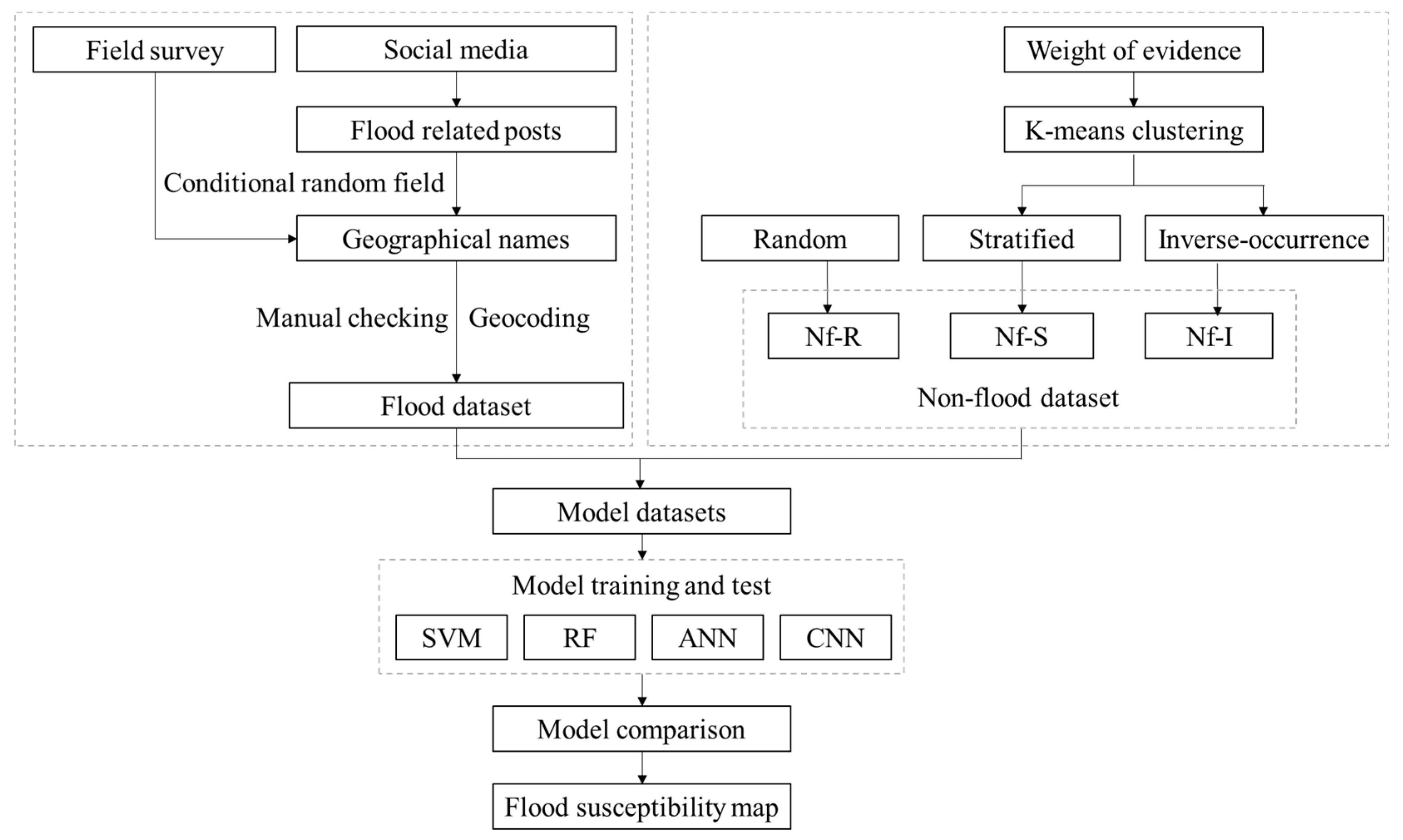
2.3. Research Framework

A flowchart of the study is shown in Figure 3. A flood inventory was built using two sources, that is, field surveys and social media. Flood records were geocoded and manually checked to ensure accuracy of flood data. For the non-flood data, random sampling was applied directly, assuming that each non-flood record had the same probability of selection. Before sampling was conducted using the stratified and inverse-occurrence approaches, all non-flood records were clustered using k-means clustering based on weight of evidence (WOE). WOE is an indicator of the connection between flood records and conditioning factors. The larger the WOE value for a subset of a conditioning factor, the stronger the subset’s linkage to flooding. Therefore, clusters derived from the WOE have a clear connection with flood probability. Subsequently, datasets composed of flood and non-flood data were input into learning models, including SVM, RF, ANN, and CNN, to produce a flood susceptibility map. For each sampling approach, 100 groups of non-flood data were used. In each group, the flood and non-flood data were divided into training (70%) and testing (30%) ten times. An average area under the receiver operating characteristic curve (AUC) for one thousand runs was used to measure the performance of the sampling approach. The most suitable models were then used to create susceptibility maps.

2.4. Non-Flood Sampling Approach

2.4.1. Random Sampling

Random sampling is a commonly used strategy for flood susceptibility mapping. Each raster grid in the study area was assumed to have the same probability of not being flooded. Therefore, non-flood points with the same number of flood points were randomly selected over the entire study area, except for the grids representing reported flood events.

2.4.2. Stratified Sampling

If the total population for sampling has significant heterogeneity among the subpopulations, it is necessary to divide the population into multiple groups that generally have maximum inter-group differences and minimum in-group differences. The number of samples extracted from a given group was then determined by the proportion of the group in the total population, such as that weighted by area. The samples extracted from distinct groups were combined to create a stratified sample. The study area was initially clustered into five groups, G1, G2, G3, G4, and G5, based on all conditioning factors, using the k-means method. This is an unsupervised classification approach that creates clusters that share similarities and are dissimilar to another cluster. Non-flood samples were generated from the five clusters in an area-weighted manner. The number of non-flood samples in Group i is calculated as follows:
M n f ( i ) = M n f × S i / i = 1 5 S i
where M n f ( i ) and S i are the number of non-flood samples and area in subpopulation i, respectively; and M n f denotes the total number of non-flood samples.

2.4.3. Inverse-Occurrence Sampling

Floods do not occur randomly over space as phenomena primarily caused by rainfall. Fluvial flooding generally affects areas surrounding river courses, whereas pluvial floods exhibit more scattered patterns [45]. Pluvial flooding can occur because of multiple factors, such as heavy rainfall, rapidly increasing impermeable surfaces, improper drainage design, pipe clogging, and local depressions. Although they have a globally sparse pattern, spatial clusters of pluvial flood events have been exemplified in case studies [46,47]. The spatial dependence of flood events is an example of the First Law of Geography. Inspired by this law, we proposed an empirical sampling strategy based on the assumption that there are more non-flood points in areas where flood events rarely occur, and vice versa. The number of non-flood samples is inversely proportional to the number of historical flood reports for each subpopulation.
The number of non-flood samples in group i is calculated as follows:
M n f ( i ) = M n f × ( M f M f ( i ) ) / i = 1 5 ( M f M f ( i ) )
where M n f ( i ) and M n f are the numbers of non-flood samples in subpopulation i and the total population, respectively; and M f ( i ) and M f denote the numbers of flood reports for subpopulation i and the total population, respectively.

2.4.4. Sampled Non-Flood Data

The two study areas were classified into five different regions (clusters), using the k-means method, and the results are presented in Table 3. The number of sampled non-flood data points in the inverse group increased as the number of flood reports decreased. However, in the stratified group, there was no clear increase or decrease in flood reports.

2.5. Learning Technique

All learning models are coded in Python 3, and hyperparameters are determined by a five-fold cross validation.

2.5.1. Support Vector Machine (SVM)

SVM is one of the most popular supervised learning algorithms. The goal is to create the most suitable hyperplane that can divide the target n-dimensional space into different classes, primarily for binary classification. The regularization factors (c) and gamma (g) were optimized using a grid-search approach on the two-dimensional plane of the two parameters. The dataset, including the flood and non-flood samples, was split into five subsets. Cross-validation was applied to assess the performance of the given c and g. After searching the entire c-g plane, the group of c (10) and g (0.0005) with the best performance was selected for the SVM model. The kernel used in this mode is a Radial Basis Function.

2.5.2. Random Forest (RF)

Random forest is an ensemble machine learning model based on multiple decision trees capable of solving classification and regression problems. This is a bagging method in which multiple random samples of data are trained independently to derive weak models. The average or most of the predictions from these weak models produced more accurate estimates. In addition to data bagging, the RF uses feature bagging to create an uncorrelated forest. Therefore, it is relatively easy for random forest to evaluate feature importance using indices such as the Gini importance and the mean decrease in impurity. Random forests have been applied to a wide range of tasks, including computer vision, finance, e-commerce, and natural hazard susceptibility analyses, yielding robust results with high accuracy. By testing multiple sets of parameter values, the optimal combination of parameters for RF was obtained, including the number of trees in the forest (200), maximum depth of trees (7), minimum number of samples required at a leaf node (5), and number of features for the best split (5).

2.5.3. Artificial Neural Network (ANN)

An ANN is a commonly used machine learning method. It comprises an input layer, one or more hidden layers, and an output layer. A training ANN was used to adjust the weights of the links connecting nodes in neighboring layers, using labeled data. In this study, two hidden layers with 400 and 450 neurons were used. The activation function is a rectified linear unit. Adam was used as the solver for the weight optimization. The maximum number of iterations, learning rate, and batch size were 1000, 0.0015, and 10, respectively.

2.5.4. Convolutional Neural Networks (CNNs)

CNNs are widely used for classification, computer vision tasks, and flood susceptibility mapping. Manual feature extraction is no longer required in a CNN; instead, linear algebra is used to identify patterns at the cost of increased computational demands. A classic CNN consists of a convolutional layer, pooling layer, and fully connected layer. The features created by the convolutional layer are input into the pooling layer for down-sampling to reduce complexity. The fully connected layer then performs classification based on the features extracted by the previous layers. We also replaced the fully connected layer with an SVM and RF for classification, resulting in three CNN models.
The feature extraction layers include a convolutional layer (output dimension, 20; kernel, 3; and padding, 1), Relu activation layer, 2 × 2 pooling layer, Relu activation layer, and fully connected layer (output dimension, 1). The classification layer is the same as that in the ANN. Adagrad was used for model optimization. The maximum number of iterations, learning rate, and batch size were 1000, 0.0015, and 10, respectively.

2.6. Model Assessment

The AUC is calculated by plotting the true-positive rate against the false-positive rate at various threshold settings. It was used to measure the predictive performance of different flood susceptibility models.

3. Results

3.1. Sampling Approach Comparison

For each machine learning method, each sampling approach was repeated 100 times with replacement, that is, bootstrapping, to create a non-flood dataset. Each sample, including flood and non-flood data, was divided ten times into a training set (70%) and a test set (30%). Therefore, there were 1000 model runs for a specific combination of learning techniques and sampling approaches, resulting in 1000 AUCs. Box plots of the AUCs for all combinations with three sampling approaches and six learning methods for Tianhe and Panyu are shown in Figure 4.
In the first case, Tianhe, the inverse-occurrence sampling significantly outperformed the other two sampling approaches, not only in terms of the AUC value but also in model robustness. In the inverse group, the mean AUC is at the level of 0.9, whereas, in random and stratified groups, they are at the level of 0.7. The AUC range in the inverse group was narrower than those in the other two groups. The AUC range is defined as the maximum AUC minus minimum AUC. The AUC ranges in the inverse group for SVM, RF, ANN, CNN, CNN-SVM, and CNN-RF were 0.15, 0.14, 0.16, 0.18, 0.15, and 0.14, respectively. The AUC ranges in the random group were 0.25, 0.28, 0.26, 0.25, 0.24, and 0.25 for SVM, RF, ANN, CNN, CNN-SVM, and CNN-RF, respectively. The AUC ranges in the stratified groups for SVM, RF, ANN, CNN, CNN-SVM, and CNN-RF were 0.23, 0.28, 0.30, 0.29, 0.24, and 0.23, respectively. This suggests that flood susceptibility models using inverse-occurrence sampling had the most stable performance.
The performances of the sampling approaches in the second case, Panyu, were consistent with those in the first case. However, the two study areas have different characteristics in terms of flood density, flood distribution, natural environment, and socioeconomic conditions. In the inverse group, the mean AUC is at the level of 0.8, whereas, in the random and stratified groups, they are at the level of 0.75. The AUC ranges in the inverse group for the SVM, RF, ANN, CNN, CNN-SVM, and CNN-RF were 0.36, 0.36, 0.39, 0.37, 0.35, and 0.38, respectively. The AUC ranges in the random group for the SVM, RF, ANN, CNN, CNN-SVM, and CNN-RF were 0.49, 0.53, 0.47, 0.43, 0.46, and 0.46, respectively. The AUC ranges in the stratified groups for SVM, RF, ANN, CNN, CNN-SVM, and CNN-RF were 0.42, 0.46, 0.48, 0.43, 0.47, and 0.46, respectively.

3.2. Learning Technique Comparison

The mean AUCs of all six machine learning techniques are listed in Table 4. To compare the performance of the learning techniques, the ranks of the learning techniques in accordance with the mean AUC were averaged for each case. In the first case, Tianhe’s CNN-RF was the most effective, followed by CNN-SVM, CNN, SVM, RF, and ANN. In the second case, Panyu exhibited the most accurate for SVM, followed by CNN-RF, RF, CNN-SVM, CNN, and ANN. Combining the two cases with distinct flood mechanisms, we found that CNN-RF was the most robust learning technique. This was followed by SVM, CNN-SVM, and RF. Although most learning approaches have different rankings in the two cases, the ANN had the least accurate performance in both cases.

3.3. Interaction between Sampling Approach and Learning Technique

The interaction between the sampling approach and learning technique determines the predictive power of the data-driven model. The larger the influence of a factor on the model performance, the larger the variation in the AUC. The variations in the AUC, which are represented by the maximum AUC minus the minimum AUC, in the sampling and learning groups are presented in Table 4. When the sampling approaches were considered as baselines, the variations caused by the learning techniques ranged from 0.0416 to 0.0930, all of which were smaller than 0.1. When the learning techniques were set as baselines, the variations caused by the sampling approaches were between 0.1487 and 0.2165, all of which were larger than 0.1. Therefore, it can be concluded that the sampling approach has a stronger influence on model performance than the learning technique. This conclusion applies to two urban areas with different flood densities, flood distributions, natural environments, and socioeconomic conditions. This includes Tianhe, with a flood density of 1.5/km2, clustered distribution, and an average slope of 9.02° in the downtown district; and Panyu, with a flood density of 0.15/km2, random distribution, and average slope of 4.55° in the suburban district.

3.4. Flood Mechanisms

In addition to data bagging, the RF uses feature bagging to create an uncorrelated forest. Therefore, in random forests, it was convenient to assess the feature importance, which is typically measured using the Gini index. In a model run, a feature was counted if its Gini index was greater than 0.1. The number of model runs in which the Gini index was ≥0.1 was counted for all twelve features in Tianhe and Panyu (Table 5). The top five features were the same in the two study areas, but in different orders. The impervious surface percentages ranked first in both cases and were larger than 0.1 in every model run. Although the newly proposed index, distance to depression, was derived using a global DEM, it ranked fifth in both cases, showing its ability to explain food mechanisms in urban districts. The spatial heterogeneity of the flood mechanism was observed in two studies. Only five features had nonzero counts in Tianhe, whereas all twelve features had at least one count in Panyu. This suggests that the floods in Panyu have more complex mechanisms than those in Tianhe. This was likely related to the relatively low flood density in Panyu (0.15) and the randomness of its spatial distribution. As shown in Table 1, the p-value for the average nearest-neighbor analysis of flood records in Panyu was 0.41. The assumption of a random flood distribution cannot be rejected at a confidence level of 95%.

3.5. Flood Susceptibility

3.5.1. Flood Density Order

Each flood susceptibility map is divided into five levels, using equal intervals: very low (0–0.2), low (0.2–0.4), moderate (0.4–0.6), high (0.6–0.8), and very high (0.8–1). The flood density in the lower-susceptibility group should be lower than that in the higher-susceptibility group. Therefore, the flood density increased in ascending order, from very low to very high. The ascending pattern was checked for all 36 best maps, comprising two study areas, three sampling approaches, and six learning techniques. The results are listed in Table 6. There were six exceptions in the ANN- and CNN-based models. This can be attributed to overfitting in the two kinds of models, leading to large areas at the very low and very high levels, as shown in the susceptibility maps in Section 3.5.3. There were no differences between the sampling approaches, and each approach had three exceptions.

3.5.2. Flood Density Outlier

The flood density in each susceptibility class varied, but it was not expected to deviate from the average flood density of the study area significantly. To compare the deviations in the two cases with different flood densities, the dimensionless relative density was defined as the flood percentage divided by the area percentage. All 180 relative densities comprising 36 maps, and 5 levels were sorted in ascending order. Empirically, a relative density greater than the 95th percentile (6.84) was considered an outlier. The number of outliers is listed in Table 7. There were six and three outliers in the CNN-RF and the RF models, respectively. Regarding the sampling approach, there were three, five, and one outlier for random sampling, stratified sampling, and inverse-occurrence sampling, respectively, suggesting that the new sampling approach is still the most robust.

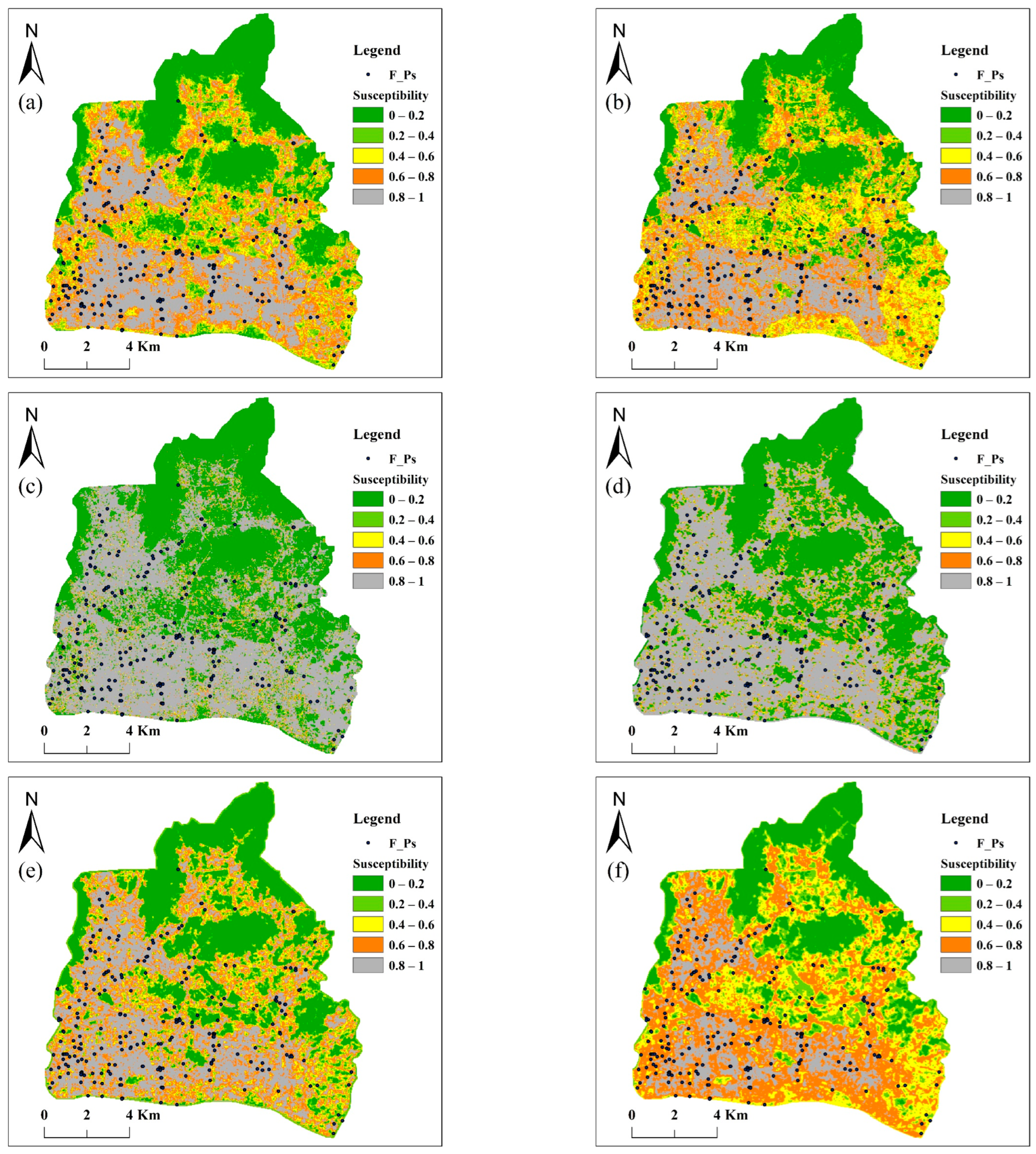
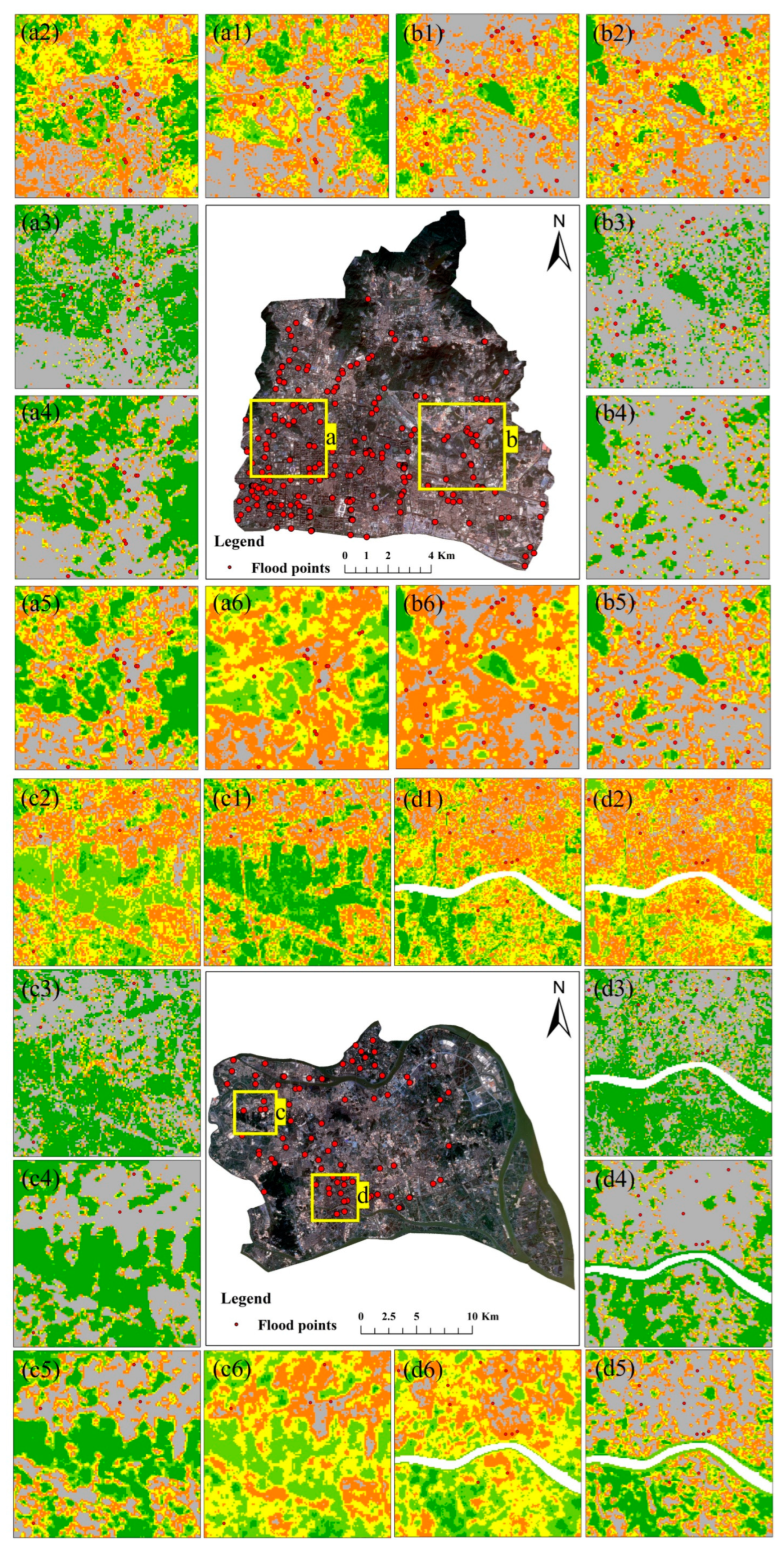
3.5.3. Flood Susceptibility Map

According to our analysis, models using inverse-occurrence sampling have the following advantages: (1) the highest AUC, (2) the maintenance of a suitable order of flood density across susceptibility levels, and (3) the least number of flood density outliers. Therefore, the most accurate models that applied inverse-occurrence sampling were used for the flood susceptibility mapping. The susceptibility maps for Tianhe and Panyu, derived using the six learning techniques, are shown in Figure 5.
The ANN- and CNN-based models exhibited clear polarized patterns in both cases. In Figure 5c,d,I,j, very low and very high values occurred for most areas, whereas the other three susceptibility levels have a limited area. The percentages of very low and very high areas were 39.8% and 50.0% for ANN in Tianhe, 37.8% and 46.8% for CNN in Tianhe, 77.6% and 15.8% for ANN in Panyu, and 75.1% and 17.2% for CNN in Panyu, respectively. The total percentages of the low, moderate, and high areas in the four models were only 10.2%, 15.4%, 6.6%, and 7.7%, respectively. Zoom-in views of flood susceptibility pattern in the two cases are also presented in Figure 6. The SVM, RF, CNN-SVM, and CNN-RF maps are capable of showing gradual gradients across all five susceptibility levels, whereas extremely steep patterns can be observed in the maps derived by ANN and CNN. These extreme patterns are related to overfitting in the learning models, which is also reflected in the ranking of the models. The ANN and CNN ranked in the last two positions in all six models. The ANN- and CNN-based models could not maintain the ascending order of flood density.

4. Discussion

4.1. Flood Susceptibility Learning in Underreported Areas

In the second case examined in this study, Panyu, the historical flood events are likely underreported. As shown in Table 1, compared to Tianhe, Panyu is three times larger in area and one and a quarter-times larger in population. In contrast, the flood events reported in Panyu (80) were only one-third of those reported in Tianhe (238). In downtown areas such as Tianhe, flood events attract public attention because of their large population density. Meanwhile, in suburban areas such as Panyu, flood information tends to propagate locally.
Unreported flood events negatively affected flood susceptibility. The number of labelled data is critical for imbalanced learning. The insufficient minority class data and flood records in this study led to a poor model performance. As shown in Figure 4, applying the inverse-occurrence sample improved the model performance for Panyu, but the improvements were limited compared to those for Tianhe. Although the AUC model can achieve an excellent level (larger than 0.9), substantial variances in the AUC suggest that the decision boundaries of the learning models in Panyu depend greatly on the data used for training. In contrast, spatial dependence was significantly rewarded in Tianhe, where the labelled data were adequate. The AUC variances were significantly reduced, and the minimum AUCs were greater than 0.8.
Two approaches can be used to enhance flood susceptibility learning in underreported areas, that is, field investigations and virtually labelled data through data augmentation. Field investigations not only effectively increase the amount of labelled data but also familiarize researchers with local flood mechanisms, which are valuable for possible model validation. A potential alternative to field investigations is data augmentation. This has been widely tested on imbalanced learning tasks, including financial fraud, intrusion detection, and medical diagnosis. Flood susceptibility mapping is a typical task for imbalanced learning. In the first case, Tianhe, flood data accounted for 0.14% of the area, although its flood density was ten times larger than that in the second case, Panyu. In future research, mainstream data augmentation techniques, including the synthetic minority oversampling technique (SMOTE), variational autoencoders (VAE), and generative adversarial networks (GAN), can be tested in underreported urban areas. Improvements caused by increased labelled data from data augmentation techniques and field investigations can be compared to determine the upper limits of data augmentation techniques.

4.2. Flood Susceptibility Model Evaluation

Indicators based on a confusion matrix, such as the AUC, accuracy, precision, recall, and F1 score, are typically used to measure the performance of machine learning models. When machine learning models are applied to a specific domain, such as flood susceptibility mapping, expert knowledge and empirical laws in that domain should be introduced as essential assessment criteria. Without these constraints, flood susceptibility maps can have excellent performance regarding general indicators based on the confusion matrix but are meaningless for guiding flood risk management.
Flood density order and outliers were used to evaluate the flood susceptibility models. It relies on two basic assumptions: flood density is positively correlated with the flood susceptibility level, and flood density has an upper limit. The first assumption is self-explanatory because the concept of flood density can be translated as the flood likelihood in a certain area. The second assumption is understandable. The flood zone occupied a relatively limited area in any watershed, whereas the flood-safe zone occupied the majority. When an extra-large outlier emerges in flood density, it is likely caused by the small area rather than the large number of flood records in a specific susceptibility class. The largest relative density in Table 7 occurred in the very high class of the CNN-RF model. In this susceptibility class, the number of flood records, flood percentage, area, and area percentage were 10, 12.5%, 0.066 km2, and 0.015%, respectively. The spatial coverage of the very high class in the model was relatively small and far below the average level. This model does not reflect the actual distribution of flood susceptibility. Therefore, it cannot be used for further susceptibility mapping, even if it works well in terms of the AUC.

4.3. Uncertainties and Limitations

Some factors related to flood formation, such as the number of storm events and drainage capability, were not included. The mean annual precipitation was used to represent the impact of the rainfall process. The number of storm events (>50 mm) is a better indicator of flood probability than the mean annual precipitation. A previous study in the same area verified that rainfall patterns dominate urban flood patterns at the city scale [47]. Unfortunately, high-resolution rainfall data were unavailable. Nevertheless, the mean annual precipitation ranked third in Tianhe and fourth in Panyu (Table 5). The drainage capacities of underground pipes, detention facilities, and pumps are key factors in preventing flooding. This was not considered in the susceptibility model, because of data availability. From this perspective, it is better to consider the flood susceptibility results as a demand for drainage and mitigation measures.
The spatial distribution of flood susceptibility was not restricted by microtopography. Precise microtopography is critical for determining detailed flood distribution. This study used ASTER GDEM, which has a spatial resolution of 30 m and vertical accuracy at the meter level. Therefore, compared with actual flood patterns, flood susceptibility patterns have uncertainties to some extent.
Limited flood records reduce the performance of deep learning models. Deep learning models such as CNN require a large amount of data for training in the computer vision domain. If the labelled data were inadequate, the models tended to overfit due to the learning noise. In the flood susceptibility mapping domain, acquiring a large number of flood records is challenging. The number of flood records used for susceptibility learning in the literature is typically at the hundred scale, and less than 300. Therefore, the three CNN models in this study showed similar performances to regular machine learning models. Nevertheless, the application of deep-learning models provided more evidence of the superiority of the newly proposed sampling approach over the two regular sampling methods.

4.4. Benefits and Future Work

In many regions, human settlement growth in the most hazardous flood zones has outpaced growth in non-exposed zones by a large margin. Middle-income countries have the largest share (81.3%) of settlements built in the highest-hazard zones [3]. In contrast with high-income countries that lead flood risk management, middle- and low-income countries always prioritize economic growth and development, which, in turn, provides financial support for flood risk management. Therefore, the flood risk evolution process tends to have an inverted U-shape similar to the Environmental Kuznets Curve (EKC) [48]. In this context, easy-to-use flood risk management tools and publicly available data are important.
This study proposed a framework for flood susceptibility assessments that use publicly available data. The framework performed well (AUC > 0.9) in two cases that were heterogeneous in terms of the natural environment, social conditions, and flood mechanisms. The newly proposed sampling strategy significantly enhances the framework, and the improvement brought about by the new sampling method is robust to multiple mainstream machine learning models and different flood mechanisms.
The application of the framework to developing regions is an important step towards Sustainable Development Goals 1 (no poverty), 9 (industry, innovation, and infrastructure), 11 (sustainable cities and communities), and 13 (climate action). Flood-induced losses can deprive low-income households of assets, pushing them back into poverty. Increasing dependency on infrastructure amplifies negative flood impacts through hazard chains. Therefore, effective and immediate actions for flood control and adaptation are required, particularly for vulnerable groups and critical infrastructure in the context of climate change.
In future research, several aspects are recommended to connect flood susceptibility to actual flood risk. First, the impact of the spatial dimension should be fully understood to capture flood mechanisms. The model dataset was always considered tabular, neglecting its spatial dimensions. Second, the heterogeneity within flood records can be considered. As a dependent variable, all flood records were assigned one. A place that is flooded once in a year cannot be compared to a place that is flooded ten times annually. Third, explainable AI is a vital aspect because it can present a clear flood mechanism that simplifies decision making on flood risk management.

5. Conclusions

This study has proposed a new sampling approach for non-flood data according to the First Law of Geography, which is also known as spatial dependence. It selects more non-flood data in areas where fewer flood events occur, and vice versa. Its performance was compared with that of two other widely favored sampling approaches, that is, random sampling and stratified sampling. To consolidate the robustness of results, a comparison was conducted using six machine learning techniques in two urban areas with different flood mechanisms in Guangzhou, China. The two urban areas have different flood densities, flood distributions, natural environments, and socioeconomic conditions, that is, Tianhe with a flood density of 1.5/km2, clustered distribution, an average slope of 9.02° in the downtown district and Panyu with a flood density of 0.15/km2, a random distribution, and an average slope of 4.55° in a suburban district. The main findings of this study are summarized as follows:
(1)
Sampling approaches have a greater impact on model performance than learning techniques. The AUC variations caused by learning techniques ranged from 0.04 to 0.09, whereas the AUC variations caused by sampling approaches were between 0.15 and 0.22 and were all larger than 0.1.
(2)
The inverse-occurrence sampling approach representing spatial dependence outperformed the two other commonly used sampling approaches, not only for high AUC values but also for small AUC variations. This finding is robust in regard to multiple learning techniques and different flooding mechanisms. AUCs in the inverse group have a narrower range, that is, 0.14–0.18 in Tianhe, and 0.35–0.39 in Panyu, than in the random group, that is, 0.24–0.28 in Tianhe, and 0.43–0.53 in Panyu; and the stratified group, which was 0.23–0.30 in Tianhe, and 0.42–0.48 in Panyu.
(3)
The most accurate learning technique measured by the AUC was CNN-RF, followed by SVM, CNN-SVM, RF, CNN, and ANN.
(4)
Flood density order and outliers should be applied to assess the quality of flood susceptibility models. ANN- and CNN-based models tended to produce polarized patterns in flood susceptibility maps, contradicting the ascending order of flood density with increasing susceptibility levels. Moreover, flood density outliers tended to appear in the models derived using RF and CNN-RF.
Flood susceptibility is not equal to the actual flood risk. It is preferable to consider flood susceptibility levels as a demand for drainage and mitigation measures. In future research, the gains from data augmentation techniques and flood record heterogeneity will be investigated. The potential of explainable AI can be explored to obtain a clear flood mechanism, rather than a black box. Finally, data-driven models should be coupled with physically based models or constrained by knowledge of local flood mechanisms to represent the actual flood risk as closely as possible.

Author Contributions

Conceptualization, H.H. and Y.L.; methodology, C.W., Y.L., W.L. and H.H.; software, C.W., Y.L., Z.T. and J.Z.; validation, C.W. and H.H.; data curation, C.W., Y.L., Z.T. and J.Z.; writing—original draft preparation, Y.L., C.W. and H.H.; writing—review and editing, all authors; supervision, H.H. All authors have read and agreed to the published version of the manuscript.

Funding

This research was supported by Guangdong Basic and Applied Basic Research Foundation (Grant #2022A1515011494) and the Science and Technology Program of Guangzhou (Grant #202201011726).

Data Availability Statement

Stream network data are available at https://www.openstreetmap.org (accessed on 12 July 2020), DEM data are available at http://asterweb.jpl.nasa.gov/ (accessed on 12 July 2020), land use data are available at https://doi.org/10.5194/essd-2023-87 (accessed on 4 May 2023), and remote sensing imageries are available at https://www.usgs.gov/landsat-missions/landsat-data-access and http://gdgf.gd.gov.cn/ (accessed on 12 July 2020).

Conflicts of Interest

The Author Yangchun Lin was employed by the Water Resources Pearl River Planning, Surveying & Designing Co., Ltd. The remaining authors declare that the research was conducted in the absence of any commercial or financial relationships that could be construed as a potential conflict of interest. The funders had no role in the design of the study; in the collection, analyses, or interpretation of data; in the writing of the manuscript; or in the decision to publish the results.

References

  1. UNDRR (United Nations Office for Disaster Risk Reduction). Human Cost of Disasters: An Overview of the Last 20 Years 2000–2019. 2020. Available online: https://www.undrr.org/publication/human-cost-disasters-overview-last-20-years-2000-2019 (accessed on 7 May 2020).
  2. Ahmad, T.; Pandey, A.C.; Kumar, A.; Tirkey, A. Understanding the role of surface runoff in potential flood inundation in the Kashmir valley, Western Himalayas. Phys. Chem. Earth 2023, 131, 103423. [Google Scholar] [CrossRef]
  3. Rentschler, J.; Avner, P.; Marconcini, M.; Su, R.; Strano, E.; Vousdoukas, M.; Hallegatte, S. Global evidence of rapid urban growth in flood zones since 1985. Nature 2023, 622, 87–92. [Google Scholar] [CrossRef] [PubMed]
  4. Delgado, C.D.; Iniestra, J.G. Flood Risk Assessment in Humanitarian Logistics Process Design. J. Appl. Res. Technol. 2014, 12, 976–984. [Google Scholar] [CrossRef]
  5. Kimuli, J.B.; Di, B.; Zhang, R.; Wu, S.; Li, J.; Yin, W. A multisource trend analysis of floods in Asia-Pacific 1990–2018: Implications for climate change in sustainable development goals. Int. J. Disaster Risk Reduct. 2021, 59, 102237. [Google Scholar] [CrossRef]
  6. Tehrany, M.S.; Pradhan, B.; Jebur, M.N. Flood susceptibility analysis and its verification using a novel ensemble support vector machine and frequency ratio method. Stoch. Environ. Res. Risk Assess. 2015, 29, 1149–1165. [Google Scholar] [CrossRef]
  7. Sahana, M.; Patel, P.P. A comparison of frequency ratio and fuzzy logic models for flood susceptibility assessment of the lower Kosi River Basin in India. Environ. Earth Sci. 2019, 78, 289. [Google Scholar] [CrossRef]
  8. Saha, S.; Sarkar, D.; Mondal, P. Efficiency exploration of frequency ratio, entropy and weights of evidence-information value models in flood vulnerabilityassessment: A study of raiganj subdivision, Eastern India. Stoch. Environ. Res. Risk Assess. 2022, 36, 1721–1742. [Google Scholar] [CrossRef]
  9. Cao, Y.; Jia, H.; Xiong, J.; Cheng, W.; Li, K.; Pang, Q.; Yong, Z. Flash Flood Susceptibility Assessment Based on Geodetector, Certainty Factor, and Logistic Regression Analyses in Fujian Province, China. ISPRS Int. J. Geo-Inf. 2020, 9, 748. [Google Scholar] [CrossRef]
  10. Tehrany, M.S.; Pradhan, B.; Jebur, M.N. Flood susceptibility mapping using a novel ensemble weights-of-evidence and support vector machine models in GIS. J. Hydrol. 2014, 512, 332–343. [Google Scholar] [CrossRef]
  11. Hong, H.; Tsangaratos, P.; Ilia, I.; Liu, J.; Zhu, A.; Chen, W. Application of fuzzy weight of evidence and data mining techniques in construction of flood susceptibility map of Poyang County, China. Sci. Total Environ. 2018, 625, 575–588. [Google Scholar] [CrossRef]
  12. Nandi, A.; Mandal, A.; Wilson, M.; Smith, D. Flood hazard mapping in Jamaica using principal component analysis and logistic regression. Environ. Earth Sci. 2016, 75, 465. [Google Scholar] [CrossRef]
  13. Ali, S.A.; Parvin, F.; Pham, Q.B.; Vojtek, M.; Vojteková, J.; Costache, R.; Linh, N.T.T.; Nguyen, H.Q.; Ahmad, A.; Ghorbani, M.A. GIS-based comparative assessment of flood susceptibility mapping using hybrid multi-criteria decision-making approach, naïve Bayes tree, bivariate statistics and logistic regression: A case of Topľa basin, Slovakia. Ecol. Indic. 2020, 117, 106620. [Google Scholar] [CrossRef]
  14. Bunmi Mudashiru, R.; Sabtu, N.; Abdullah, R.; Saleh, A.; Abustan, I. Optimality of flood influencing factors for flood hazard mapping: An evaluation of two multi-criteria decision-making methods. J. Hydrol. 2022, 612, 128055. [Google Scholar] [CrossRef]
  15. Vilasan, R.T.; Kapse, V.S. Evaluation of the prediction capability of AHP and F-AHP methods in flood susceptibility mapping of Ernakulam district (India). Nat. Hazards 2022, 112, 1767–1793. [Google Scholar] [CrossRef]
  16. Kanani-Sadat, Y.; Arabsheibani, R.; Karimipour, F.; Nasseri, M. A new approach to flood susceptibility assessment in data-scarce and ungauged regions based on GIS-based hybrid multi criteria decision-making method. J. Hydrol. 2019, 572, 17–31. [Google Scholar] [CrossRef]
  17. Gudiyangada Nachappa, T.; Tavakkoli Piralilou, S.; Gholamnia, K.; Ghorbanzadeh, O.; Rahmati, O.; Blaschke, T. Flood susceptibility mapping with machine learning, multi-criteria decision analysis and ensemble using Dempster Shafer Theory. J. Hydrol. 2020, 590, 125275. [Google Scholar] [CrossRef]
  18. Rafiei-Sardooi, E.; Azareh, A.; Choubin, B.; Mosavi, A.H.; Clague, J.J. Evaluating urban flood risk using hybrid method of TOPSIS and machine learning. Int. J. Disaster Risk Reduct. 2021, 66, 102614. [Google Scholar] [CrossRef]
  19. Chen, Y. Flood hazard zone mapping incorporating geographic information system (GIS) and multi-criteria analysis (MCA) techniques. J. Hydrol. 2022, 612, 128268. [Google Scholar] [CrossRef]
  20. Zhao, G.; Pang, B.; Xu, Z.; Yue, J.; Tu, T. Mapping flood susceptibility in mountainous areas on a national scale in China. Sci. Total Environ. 2018, 615, 1133–1142. [Google Scholar] [CrossRef]
  21. Norallahi, M.; Seyed Kaboli, H. Urban flood hazard mapping using machine learning models: GARP, RF, MaxEnt and NB. Nat. Hazards 2021, 106, 119–137. [Google Scholar] [CrossRef]
  22. Tang, X.; Machimura, T.; Liu, W.; Li, J.; Hong, H. A novel index to evaluate discretization methods: A case study of flood susceptibility assessment based on random forest. Geosci. Front. 2021, 12, 101253. [Google Scholar] [CrossRef]
  23. Mangukiya, N.K.; Sharma, A. Flood risk mapping for the lower Narmada basin in India: A machine learning and IoT-based framework. Nat. Hazards 2022, 113, 1285–1304. [Google Scholar] [CrossRef]
  24. Xiong, J.; Li, J.; Cheng, W.; Wang, N.; Guo, L. A GIS-Based Support Vector Machine Model for Flash Flood Vulnerability Assessment and Mapping in China. ISPRS Int. J. Geo-Inf. 2019, 8, 297. [Google Scholar] [CrossRef]
  25. Zhao, G.; Pang, B.; Xu, Z.; Peng, D.; Xu, L. Assessment of urban flood susceptibility using semi-supervised machine learning model. Sci. Total Environ. 2019, 659, 940–949. [Google Scholar] [CrossRef] [PubMed]
  26. Sahana, M.; Rehman, S.; Sajjad, H.; Hong, H. Exploring effectiveness of frequency ratio and support vector machine models in storm surge flood susceptibility assessment: A study of Sundarban Biosphere Reserve, India. Catena 2020, 189, 104450. [Google Scholar] [CrossRef]
  27. Andaryani, S.; Nourani, V.; Haghighi, A.T.; Keesstra, S. Integration of hard and soft supervised machine learning for flood susceptibility mapping. J. Environ. Manag. 2021, 291, 112731. [Google Scholar] [CrossRef]
  28. Chen, W.; Li, Y.; Xue, W.; Shahabi, H.; Li, S.; Hong, H.; Wang, X.; Bian, H.; Zhang, S.; Pradhan, B.; et al. Modeling flood susceptibility using data-driven approaches of naïve Bayes tree, alternating decision tree, and random forest methods. Sci. Total Environ. 2020, 701, 134979. [Google Scholar] [CrossRef]
  29. Tang, X.; Li, J.; Liu, M.; Liu, W.; Hong, H. Flood susceptibility assessment based on a novel random Naïve Bayes method: A comparison between different factor discretization methods. Catena 2020, 190, 104536. [Google Scholar] [CrossRef]
  30. Khosravi, K.; Panahi, M.; Golkarian, A.; Keesstra, S.D.; Saco, P.M.; Bui, D.T.; Lee, S. Convolutional neural network approach for spatial prediction of flood hazard at national scale of Iran. J. Hydrol. 2020, 591, 125552. [Google Scholar] [CrossRef]
  31. Wang, Y.; Fang, Z.; Hong, H.; Peng, L. Flood susceptibility mapping using convolutional neural network frameworks. J. Hydrol. 2020, 582, 124482. [Google Scholar] [CrossRef]
  32. Zhao, G.; Pang, B.; Xu, Z.; Peng, D.; Zuo, D. Urban flood susceptibility assessment based on convolutional neural networks. J. Hydrol. 2020, 590, 125235. [Google Scholar] [CrossRef]
  33. Saha, S.; Gayen, A.; Bayen, B. Deep learning algorithms to develop Flood susceptibility map in Data-Scarce and Ungauged River Basin in India. Stoch. Environ. Res. Risk Assess. 2022, 36, 3295–3310. [Google Scholar] [CrossRef]
  34. Ullah, K.; Wang, Y.; Fang, Z.; Wang, L.; Rahman, M. Multi-hazard susceptibility mapping based on Convolutional Neural Networks. Geosci. Front. 2022, 13, 101425. [Google Scholar] [CrossRef]
  35. Shahabi, H.; Shirzadi, A.; Ronoud, S.; Asadi, S.; Pham, B.T.; Mansouripour, F.; Geertsema, M.; Clague, J.J.; Bui, D.T. Flash flood susceptibility mapping using a novel deep learning model based on deep belief network, back propagation and genetic algorithm. Geosci. Front. 2021, 12, 101100. [Google Scholar] [CrossRef]
  36. Fang, Z.; Wang, Y.; Peng, L.; Hong, H. Predicting flood susceptibility using LSTM neural networks. J. Hydrol. 2021, 594, 125734. [Google Scholar] [CrossRef]
  37. Al-Abadi, A.M.; Pradhan, B. In flood susceptibility assessment, is it scientifically correct to represent flood events as a point vector format and create flood inventory map? J. Hydrol. 2020, 590, 125475. [Google Scholar] [CrossRef]
  38. Fang, L.; Huang, J.; Cai, J.; Nitivattananon, V. Hybrid approach for flood susceptibility assessment in a flood-prone mountainous catchment in China. J. Hydrol. 2022, 612, 128091. [Google Scholar] [CrossRef]
  39. Tang, X.; Li, J.; Liu, W.; Yu, H.; Wang, F. A method to increase the number of positive samples for machine learning-based urban waterlogging susceptibility assessments. Stoch. Environ. Res. Risk Assess. 2022, 36, 2319–2336. [Google Scholar] [CrossRef]
  40. Ekmekcioğlu, Ö.; Koc, K.; Özger, M.; Işık, Z. Exploring the additional value of class imbalance distributions on interpretable flash flood susceptibility prediction in the Black Warrior River basin, Alabama, United States. J. Hydrol. 2022, 610, 127877. [Google Scholar] [CrossRef]
  41. Dodangeh, E.; Choubin, B.; Eigdir, A.N.; Nabipour, N.; Panahi, M.; Shamshirband, S.; Mosavi, A. Integrated machine learning methods with resampling algorithms for flood susceptibility prediction. Sci. Total Environ. 2020, 705, 135983. [Google Scholar] [CrossRef]
  42. Tang, X.; Hong, H.; Shu, Y.; Tang, H.; Li, J.; Liu, W. Urban waterlogging susceptibility assessment based on a PSO-SVM method using a novel repeatedly random sampling idea to select negative samples. J. Hydrol. 2019, 576, 583–595. [Google Scholar] [CrossRef]
  43. Rajabi, A.; Shabanlou, S.; Yosefvand, F.; Kiani, A. Exploring the sample size and replications scenarios effect on spatial prediction of flood, using MARS and MaxEnt methods case study: Saliantape catchment, Golestan, Iran. Nat. Hazards 2021, 109, 871–901. [Google Scholar] [CrossRef]
  44. Tobler, W.R. A Computer Movie Simulating Urban Growth in the Detroit Region. Econ. Geogr. 1970, 46, 234–240. [Google Scholar] [CrossRef]
  45. Winters, B.A.; Angel, J.R.; Ballerine, C.; Byard, J.; Flegel, A.; Gambill, D.; Jenkins, E.; McConkey, S.A.; Markus, M.; Bender, B.A.; et al. Report for the Urban Flooding Awareness Act; Illinois Department of Natural Resources: Springfield, IL, USA, 2015. [Google Scholar]
  46. Cherqui, F.; Belmeziti, A.; Granger, D.; Sourdril, A.; Le Gauffre, P. Assessing urban potential flooding risk and identifying effective risk-reduction measures. Sci. Total Environ. 2015, 514, 418–425. [Google Scholar] [CrossRef] [PubMed]
  47. Huang, H.; Chen, X.; Zhu, Z.; Xie, Y.; Liu, L.; Wang, X.; Wang, X.; Liu, K. The changing pattern of urban flooding in Guangzhou, China. Sci. Total Environ. 2018, 622–623, 394–401. [Google Scholar] [CrossRef] [PubMed]
  48. Huang, H.; Pan, Y.; Wang, C.; Wang, X. Nonlinear Flood Responses to Tide Level and Land Cover Changes in Small Watersheds. Land 2023, 12, 1743. [Google Scholar] [CrossRef]
Figure 1. Study areas: (a) Guangzhou, (b) Tianhe, and (c) Panyu. In the subgraph (a), “Y”, “L”, “HZ”, and “TH” mean Yuexiu, Liwan, Haizhu, and Tianhe district. The land cover is represented by Gaofen 1 satellite imagery, using false color.
Remotesensing 15 05384 g001
Figure 2. Conditioning factors in the two study areas, that is, Tianhe (1) and Panyu (2). The subgraphs are (a) elevation, (b) slope, (c) relative elevation, (d) standard deviation of elevation, (e) distance to depression, (f) impervious surface percentage, (g) normalized difference vegetation index, (h) normalized difference built-up index, (i) distance to river, (j) rainfall, (k) topographic wetness index, and (l) stream power index.
Remotesensing 15 05384 g002aRemotesensing 15 05384 g002bRemotesensing 15 05384 g002c
Figure 3. Flowchart of data preparation and model comparison on flood susceptibility mapping. Nf-R, Nf-S, and Nf-I denote non-flood datasets created using random sampling, stratified sampling, and inverse-occurrence sampling, respectively.
Remotesensing 15 05384 g003
Figure 4. Box plots of AUC for the three sampling strategies controlled by six learning approaches. (af) were controlled by SVM, RF, ANN, CNN, CNN-SVM, and CNN-RF, respectively, in Tianhe. (gl) were conditional on SVM, RF, ANN, CNN, CNN-SVM, and CNN-RF, respectively, in Panyu. The dashed lines represent the mean AUCs. “Random”, “Stratified”, and “Inverse” represent random sampling, stratified sampling, and inverse-occurrence sampling, respectively.
Remotesensing 15 05384 g004
Figure 5. Flood susceptibility maps using inverse-occurrence sampling. (af) Maps of Tianhe, learned using SVM, RF, ANN, CNN, CNN-SVM, and CNN-RF, respectively. (gl) Maps of Panyu, learned using SVM, RF, ANN, CNN, CNN-SVM, and CNN-RF, respectively. F_Ps, flood points.
Remotesensing 15 05384 g005aRemotesensing 15 05384 g005b
Figure 6. Zoom-in views of flood susceptibility pattern in Tianhe (a,b) and Panyu (c,d). The subgraphs are (1) SVM, (2) RF, (3) ANN, (4) CNN, (5) CNN-SVM, and (6) CNN-RF, respectively.
Remotesensing 15 05384 g006
Table 1. Information on the two study areas.
Study AreaFlood
Records
Area
(km2)
Flood Density (1/km2)Cluster Analysis
(p-Value)
Population 2021
(Million)
GDP 2021
(Billion Yuan)
Average Slope
(Degree)
Tianhe238158.351.500.002.24601.29.02
Panyu80516.340.150.412.82265.44.55
Table 2. Data description.
DataSourceFormatResolution
Stream networkOpen street mapPolyline, shape file-
Land useSinoLC-1, 2023Raster1 m
DEMASTER GDEMRaster30 m
Remote sensing imageryLandsat 8, 2020Raster30 m
Gaofen 1, 2020Raster8 m
Table 3. Cluster results and the number of non-flood data points.
ClustersFlood NumberFlood Percentage (%)Area Percentage (%)Non-Flood Number (Inverse)Non-Flood Number (Stratified)
Tianhe117171.840.81797
25824.433.24579
383.48.45720
410.410.55925
500.07.16017
Panyu14455.018.3914
22733.823.41319
378.822.81818
411.320.82017
511.314.82012
Table 4. Mean AUC and its ranking for six learning techniques. AUC change S and L denote the changes in AUC caused by the sampling approach and learning technique, respectively. “—” means not applicable.
MethodTianhePanyuAverage
Rank
AUC Change S
RandomStratifiedInverseRankRandomStratifiedInverseRank
SVM0.69740.70370.90184.00.78280.78240.83921.02.50.2044
RF0.69490.69830.91144.00.76250.75790.82433.03.50.2165
ANN0.66360.66530.87606.00.71860.71640.78276.06.00.2124
CNN0.73590.73820.88463.70.75100.74700.80475.04.30.1487
CNN-SVM0.74030.74200.90652.30.76080.75650.81554.03.20.1662
CNN-RF0.75430.75830.91761.00.77480.77370.82742.01.50.1633
AUC change L0.09070.09300.04160.06420.06600.0565
Table 5. Feature ranking in RF models using inverse-occurrence sampling (Gini index ≥ 0.1).
TianhePanyu
ISP1000ISP1000
NDVI1000Elevation461
Rainfall358NDVI436
Elevation41Rainfall92
DD40DD81
DR0DR46
NDBI0NDBI18
RE0STDE12
Slope0RE10
SPI0Slope8
STDE0SPI1
TWI0TWI1
Table 6. Flood density in the ascending order: true (√) or false (×).
Study AreaSampling ApproachSVMRFANNCNNCNN-SVMCNN-RF
TianheRandom×
Stratified××
Inverse×
PanyuRandom××
Stratified×
Inverse××
Table 7. The number of relative density outliers (>6.84, dimensionless). Outlier values are listed within the parentheses after the number. ‘—’ means no outlier. Absolute flood densities (1/km2) in two cases are also given.
Study AreaSampling ApproachSVMRFANNCNNCNN-SVMCNN-RF
Tianhe
(1.5/km2)
Random1 (7.89)1 (239.2)
Stratified1 (17.82)2 (7.27, 575.05)
Inverse
Panyu
(0.15/km2)
Random1 (262.55)
Stratified1 (8.18)1 (848.8)
Inverse1 (13.61)
Disclaimer/Publisher’s Note: The statements, opinions and data contained in all publications are solely those of the individual author(s) and contributor(s) and not of MDPI and/or the editor(s). MDPI and/or the editor(s) disclaim responsibility for any injury to people or property resulting from any ideas, methods, instructions or products referred to in the content.

