3.1. Cryosat-2 vs. Concurrent Altimetry
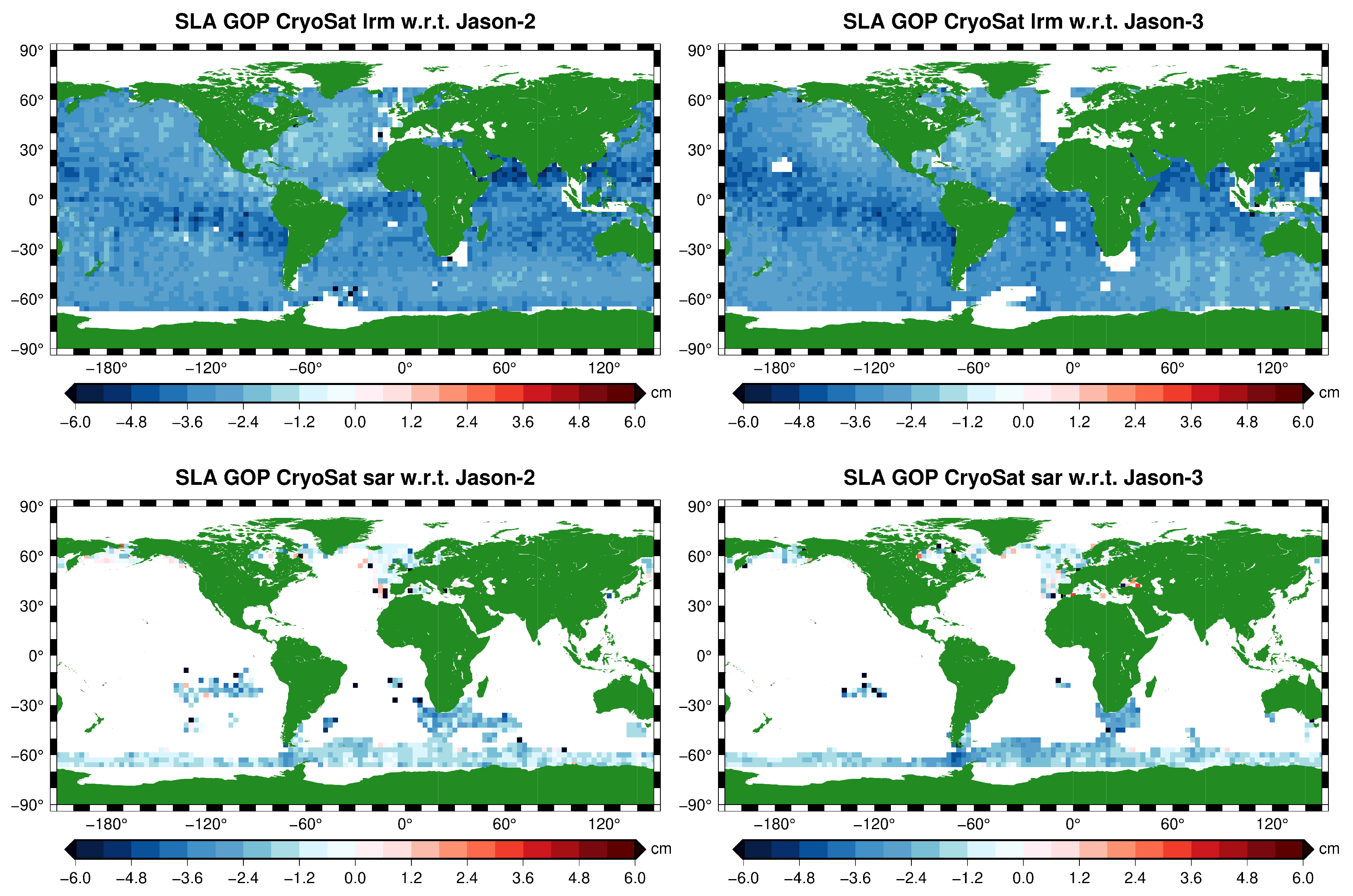
Figure 6 gives the result for mean crossover difference for sea level anomaly (SLA) between GOP Cryosat-2 and all the other concurrent altimeter satellite missions/phases. Due to CryoSat-2’s orbit, the number of crossovers within
days is limited, which results in a typical banded pattern for the case where GOP CryoSat-2 crosses RADS CryoSat-2. Consecutively,
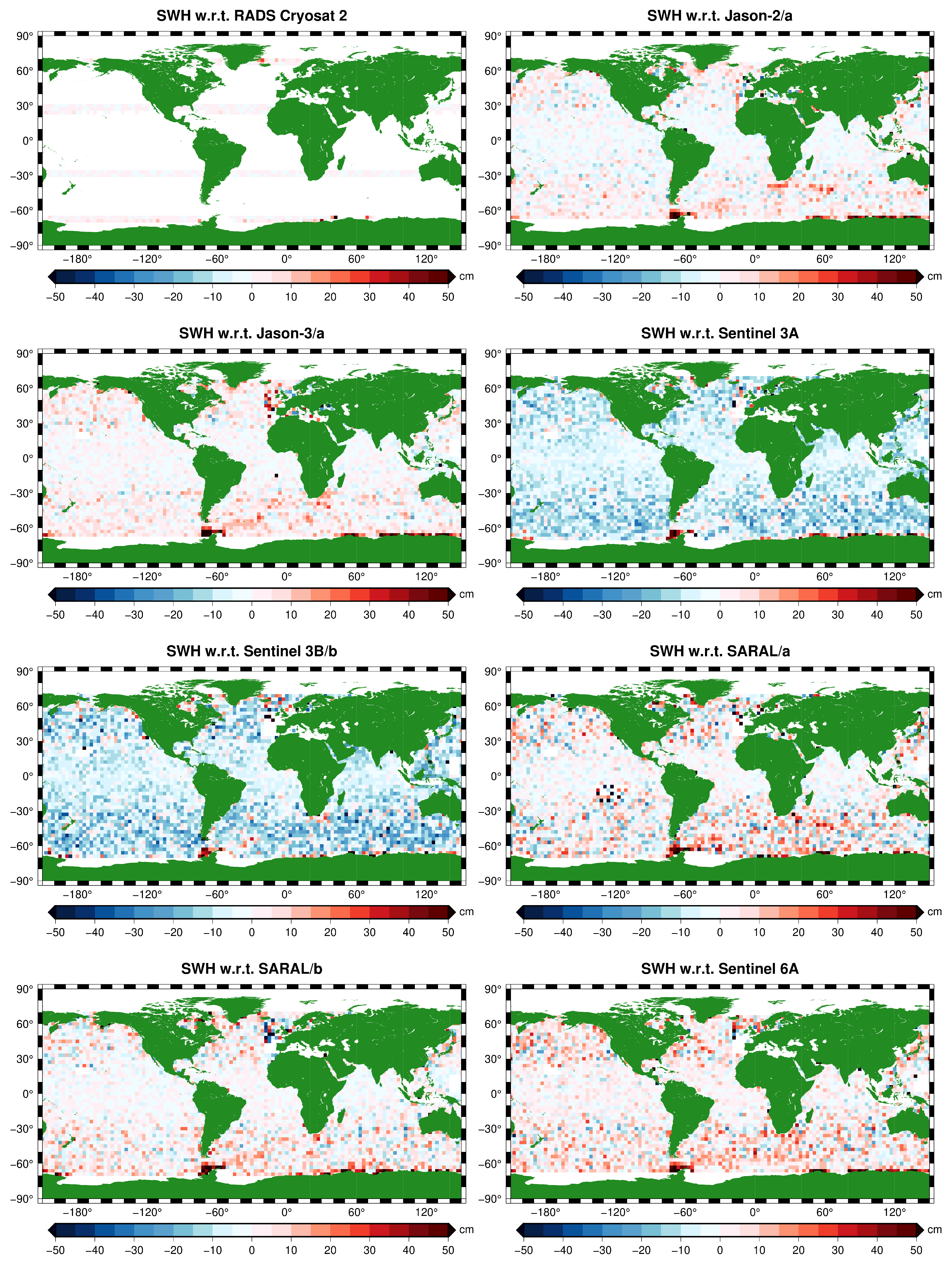
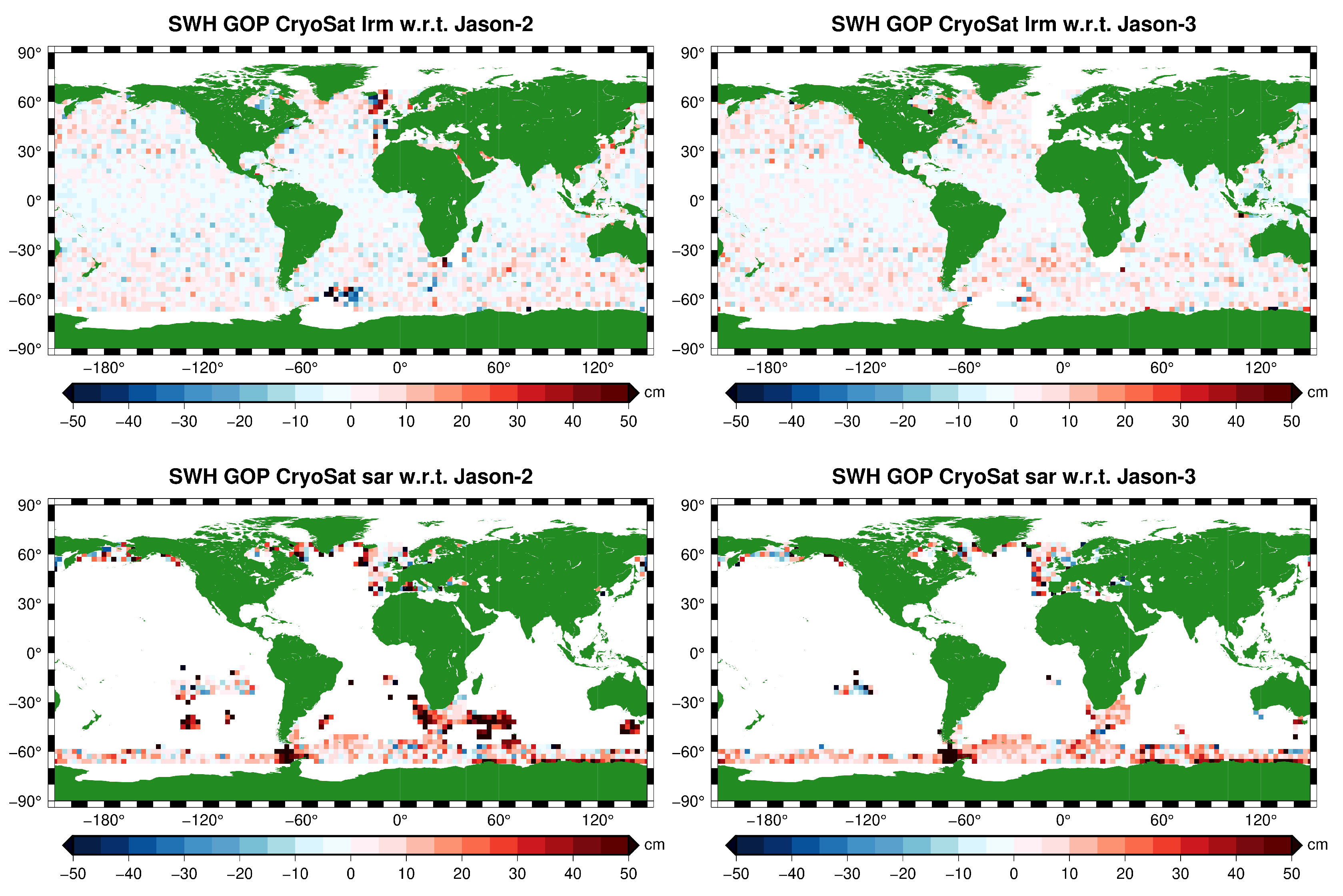
Figure 7 gives the mean crossover difference for significant wave height (SWH) between GOP CryoSat-2 and the other altimeter satellites, and
Figure 8 gives the wind speed (WIND). In the
Supplementary Materials, Figures S1 and S2 give the results for backscatter (
) and sea state bias (SSB), respectively. All these plots give insight on how the biases are distributed geographically. Obviously, they are averaged over the period in which the two crossing satellites overlap (
Table 1).
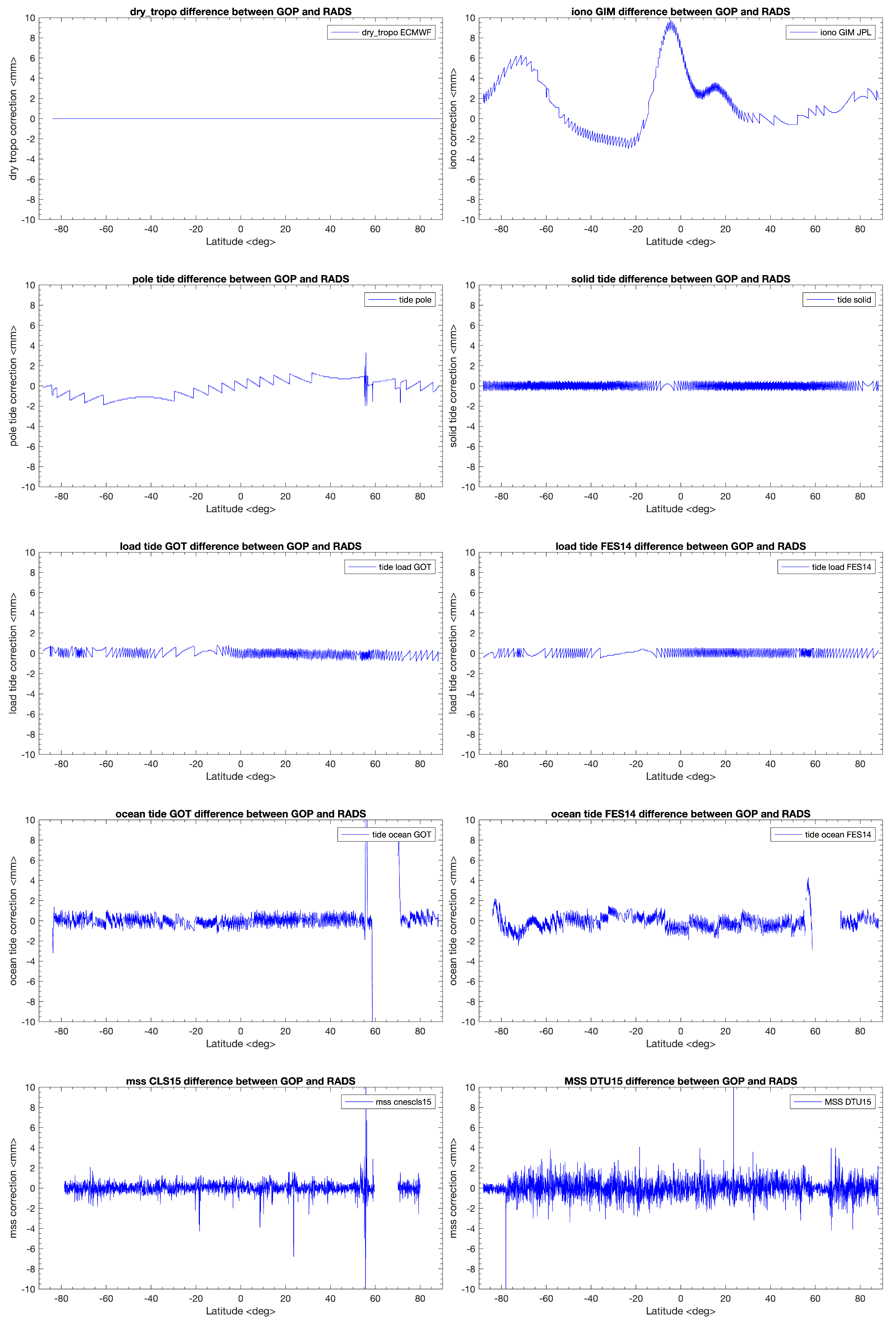
A few immediately striking observations from these figures can be made: In the SLA (
Figure 6), we see, for all satellite comparisons, a returning SLA difference pattern around the equator, which we have already seen in
Section 2.2,
Figure 3, i.e., an enhanced meandering band following the inclination of the magnetic field, hinting at our ionosphere correction ‘problem’, as well as an average bias close to −3 cm. In the significant wave height SWH (
Figure 7), large departures from the Sentinels and SARAL, and in the wind speed (
Figure 8), typical banded differences (polar regimes), though they are absent in the differences from the SARALs.
In
Figure 9, in the left panel, we plot the mean crossover difference SLA for crossing RADS CryoSat-2 with Jason-2/a and see that the equator band has more or less disappeared when compared with the GOP CryoSat-2 with the Jason-2/a solution (
Figure 6, top right panel). We also applied the −2.9 cm bias to this solution, so it can be readily compared. In the right panel of
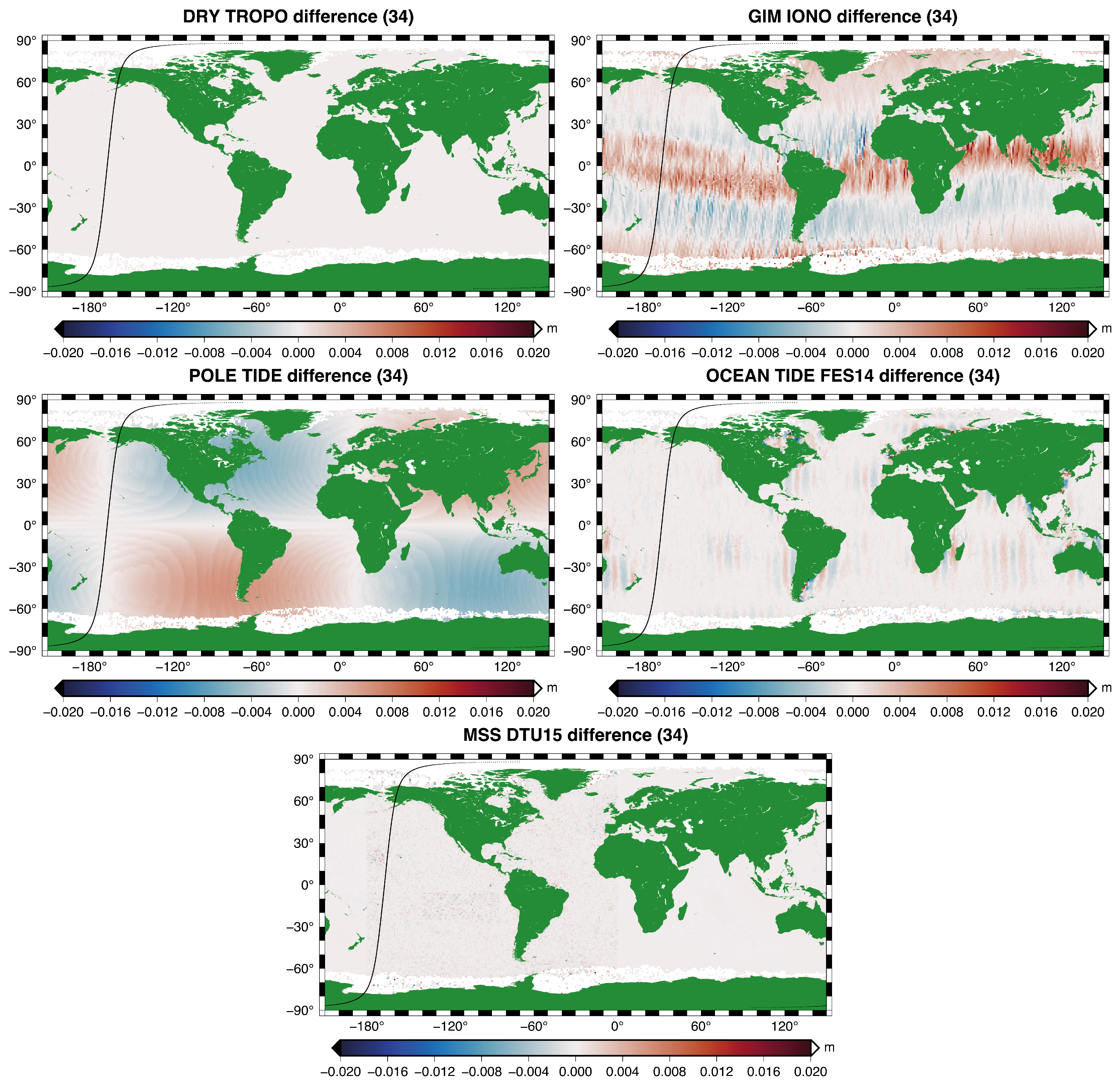
Figure 9, we compare both solutions (subtracting the GOP solution from the RADS solution). In this manner, we found a way to directly compare GOP CryoSat-2 with RADS CryoSat-2 crossovers with full geographical coverage without being bothered by any range bias (it cancels out in the comparison). Obviously, this difference between RADS CryoSat-2 and GOP CryoSat-2 is a combination of the GIM ionosphere correction (equatorial band) and pole tide correction difference (a typical degree 2, order 1, Legendre polynomial pattern), as seen in
Figure 3 in the top right and center left panels. From this, we conclude that the ‘problem’ of the ionosphere is in either all RADS data or just in the GOP data, and this agrees with the observation in
Section 2.2 that we are dealing with different implementations of the GIM ionosphere correction model.
Table 4a provides the overall crossover statistics from the dual-satellite crossover analyses: obviously, they match with
Figure 6,
Figure 7 and
Figure 8, and we added the statistics for backscatter (
) and sea state bias (SSB). Finally,
Table 4b provides, for the same data products and data fields, the single-satellite crossover statistics. The last column in the tables provides the number of crossovers involved (after editing). We conclude that the GOP CryoSat-2 product is of similar quality as the Jasons, and it also closely follows the Sentinels and SARAL. The only difference standing out when going back to
Table 4a is the average SLA (absolute) range bias of −2.9 cm, which is based on the average GOP SLA differences with the other satellites that have the longest phases, but leaving out SARAL, which has another type of altimeter instrument, and leaving out Sentinel-6A, which has too much of a deviating SLA XO mean. Knowing that for baseline-B we found −6.3 cm, we conclude that the GOP product absolute bias has been improved by 3.4 cm by a welcome change in ground processing. The overall sd of GOP XO differences is established at 3.7 cm, perfectly on par with the internal consistency (sd) of Jason-2 and Jason-3. Also, we see important improvements in the average biases for
and wind speed. All in all, the statistics for Baseline-C improved substantially upon an already well-performing Baseline-B product.
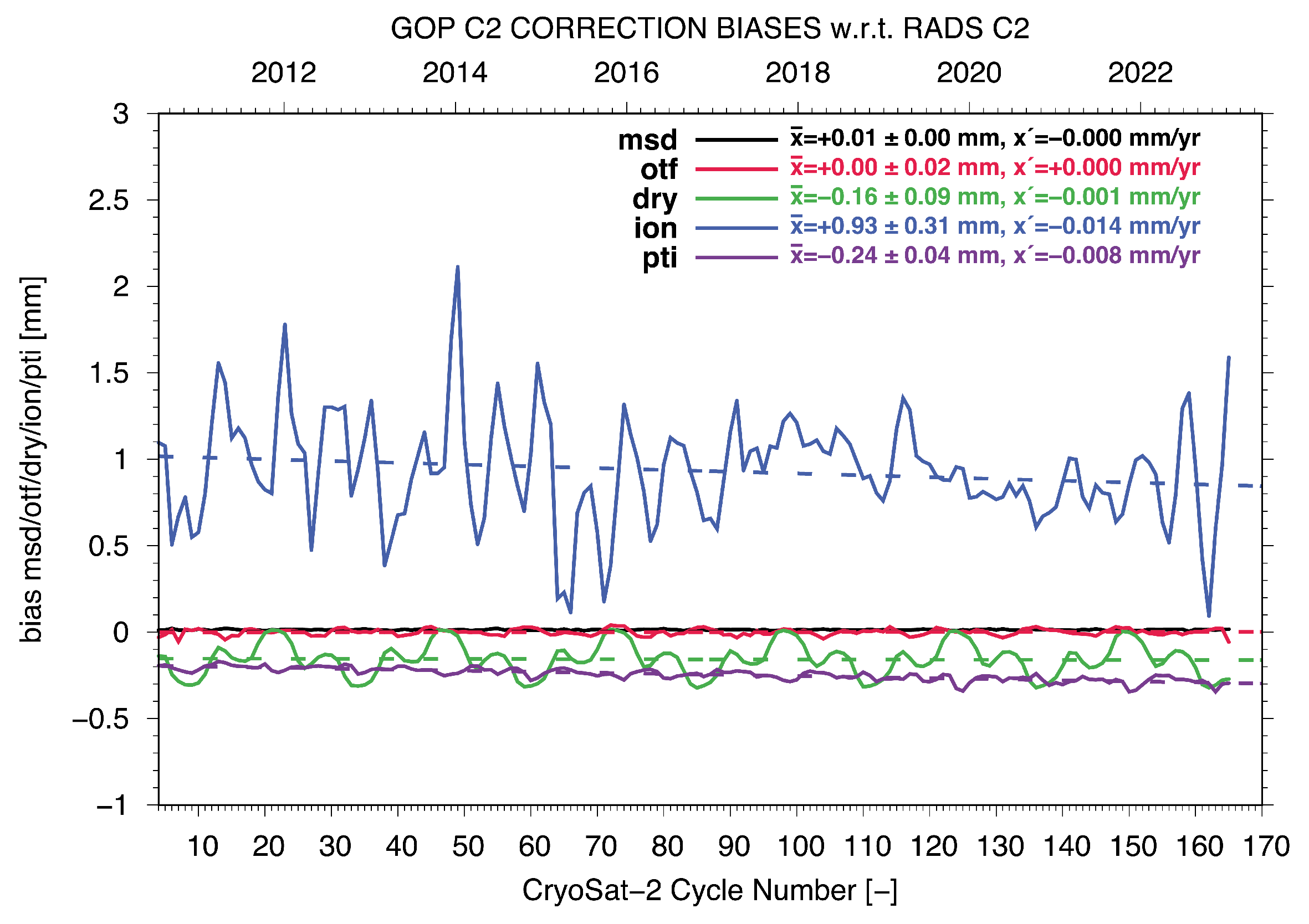
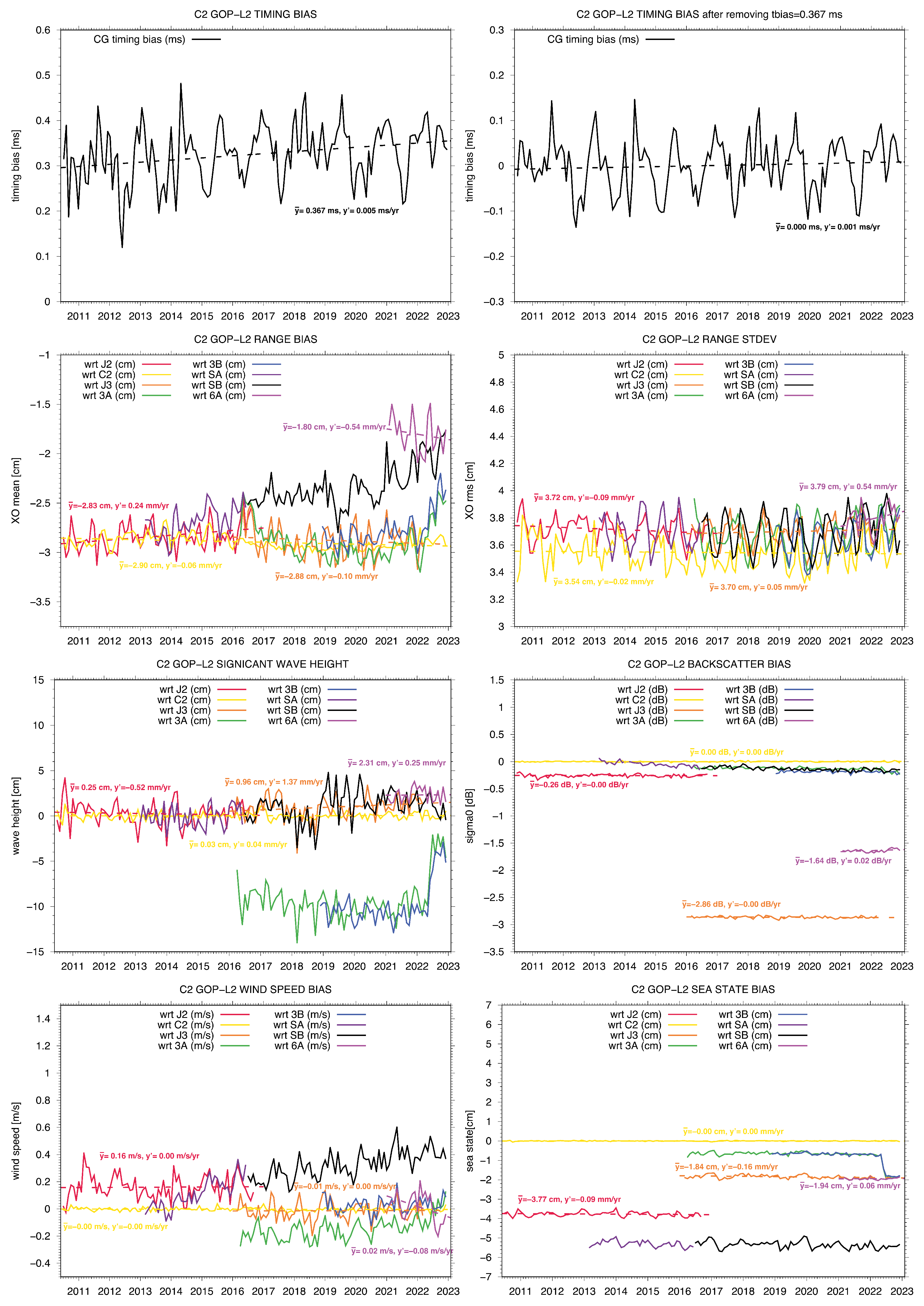
Let us now take a closer look at the different biases and how they evolve over time. In
Figure 10, we plotted, from left to right and from top to bottom, the monthly global averages from our dual-satellite crossover analyses (mean XO differences) for seven altimetric parameters: the timing bias, the sea level anomaly (range) bias, the SLA bias standard deviation (rms XO differences), significant wave height (SWH) bias, backscatter (
) bias, wind speed bias, and sea state bias (SSB). For the GOP CryoSat-2 biases with respect to the reference missions (Jason-2, Jason-3, and Sentinel-6A) and with respect to RADS CryoSat-2, the values of the long-term average and trends are given in, respectively, red, orange, pink, and yellow. Obviously, the long-term averages match the values in
Table 4a. The timing bias, based on minimization of the rms of GOP CryoSat single XO differences (more details in [
12]), has an overall average of +0.367 ms with a slight rise over time (
Figure 10, top left), which averages to zero when this is applied to the GOP data (
Figure 10, top right). This is a change compared with the result from our Baseline-B analyses, indicating a change in the ground processing. In the left panel of the 2nd row of
Figure 10, we see the SLA mean crossover difference in GOP CryoSat-2 with respect to Jason-2 (red curve, average of
cm), with respect to RADS CryoSat-2 (yellow curve, average of
cm), with respect to Jason-3 (orange curve, average of
cm), with respect to Sentinel-6A (pink curve, average of
cm), and with respect to the other satellites (Sentinel-3A and 3B, respectively, green and blue curves, and SARAL phase a and b, respectively, purple and black curves). With all this information, we can pinpoint the absolute range bias of the GOP data at
cm. The drift in the range bias with respect to Jason-2 amounts to 0.24 mm/yr, with respect to Jason-3 to
mm/yr, with respect to RADS CryoSat to
mm/yr, and with respect to Sentinel-6A to
mm/yr. Taking into account that the GOP-RADS difference basically only hints at ‘problematic’ range corrections (and not to the altimeter or platform itself), and that for Sentinel-6A, the time span is too short for a statement on the long term, we can say that compared with Jason-2 and Jason-3, GOP CryoSat-2 Baseline-C is excellently stable over time (averaging −0.07 mm/yr) and significantly better than the constraint of 0.5 mm/yr for an altimeter to have SLA considered an essential climate variable ECV (
https://climate.esa.int/en/evidence/what-are-ecvs, accessed on 1 September 2023). In the dual XO rms (right plot, second row), we see the confirmation of the quality of the stability, averaging 3.7 cm, in line with the internal consistency of our Jason-2 and Jason-3 reference missions (compare with
Table 4b). The stability is also on par with the current general uncertainty in sea level trend estimates (<0.4 mm/yr). All the mean biases, either in SLA, SWH,
, wind speed, or SSB, confirm the earlier figures and tables. Obviously, there are jumps in
and wind speed when, for instance, switching from Jason-2 to Jason-3. Basically, that is not of direct concern for the GOP product because any jumps in
and, by that, in wind speed, are ’fixed’ (discounted) in the optimized sea state bias model.
Knowing that GOP is quite stable, CryoSat-2 can function as a stable reference as well for other satellites, for instance, for the two SARAL phases a and b and for Sentinel-6A. From the tables and
Figure 10, we learn that GOP has a range bias of
cm and that the average bias between GOP and Sentinel-6A is
cm, thus subtracting the
cm from the
cm gives Sentinel-6A the absolute range bias of
cm (also because in RADS there is no range bias established yet, and nothing (0 cm) is applied in RADS to Sentinel-6A by default). Applying this
cm absolute bias value to the Sentinel-6A data, we can extend our reference mission series Jason-2/Jason-3 to Jason-2/Jason-3/Sentinel-6A.
The large positive trends in the SARAL phases a and b SLA with respect to GOP, and also with respect to Jason-2 and Jason-3, in the left panel of the second row of
Figure 10 are worrying. So, this seems to be an isolated problem in the SARAL data. We think these results warrant further research into the SARAL altimeter data. This is out of the scope of this paper, but we see similar behavior in the backscatter (negative trend) and wind speed (positive trend). Another concern is the SLA difference in GOP and Sentinel-3A and Sentinel-3B that suddenly starts rising halfway through 2022. The direct question of course would be if there is something wrong with the GOP data after this date. Whereas the difference in GOP SLA with respect to Jason-2, Jason-3, and even Sentinel-6A, doe not show this behavior and hints to a problem with the Sentinel-3 data, the actual answer comes from the wave height plot and the sea state plot of
Figure 10:, revealing jumps in Sentinel-3A and Sentinel-3B data of 6 cm in wave height and 1 cm in sea state bias, starting approximately in June 2022. Again, with the help of GOP CryoSat-2 data, another altimeter problem has been uncovered. To be absolutely sure that there is no degradation of GOP CryoSat-2 after 2022, we performed an extra analysis with respect to a selected set of PSMSL tide gauges, for which the reader is referred to
Section 3.3.1. The overall conclusion is that CryoSat-2 GOP has no apparent drift with respect to tide gauge sea levels, not even after 2022 upon close inspection.
A final remark on the range bias between the two CrySat-2 products, the GOP and the RADS version, which we already stated that in essence only deals with the correction differences: from the green curve in the left hand plot of the 2nd row of
Figure 10, we observe a negligible trend (
mm/yr), concluding that both the ionosphere correction and pole tide correction issues do not degrade CryoSat’s stability whatsoever.
3.2. CryoSat Modes and Descending/Ascending Pass Bias
As we mixed LRM and SAR mode in our previous bias analyses, it is interesting to reanalyze the bias but now separated into CryoSat’s Low-Resolution Mode (LRM) and Synthetic Aperture Radar (SAR) mode. In
Figure 11,
Figure 12 and
Figure 13, we plotted similar geographical maps of the mean crossovers of CryoSat-2 GOP (only with respect to Jason-2 and Jason-3), as in
Figure 6,
Figure 7 and
Figure 8, but now for the two different modes, respectively, for sea level anomaly SLA, significant wave height SWH, and wind speed WIND. Obviously, the LRM solutions resemble the earlier combination of LRM and SAR, as the SAR mode is geographically limited. The thing to notice here is the differences between the LRM solutions and SAR solutions. For instance, in
Figure 11, we see that the SLA mean XO differences on average are lighter blue for SAR than for LRM, indicating a bias between LRM and SAR SLA (positive when subtracting LRM from SAR). We observe something similar for the wind speed (
Figure 13), but it is less prominent, and again, it is more pronounced for the significant wave height (
Figure 12) (darker red for SAR, meaning a positive bias subtracting LRM from SAR). The main purpose of these geographical distribution maps is to see whether there are striking patterns. For this, we refer the reader back to our earlier maps and discussion on ’all’ (LRM plus SAR) solutions in the previous section.
To obtain some statistics on the mode biases, we again investigate their evolution over time. In
Figure 14, we plotted, from left to right and from top to bottom, the monthly global averages from our dual-satellite crossover analyses (mean XO differences) for four altimetric parameters: the sea level anomaly (range) bias, the significant wave height (SWH) bias, the wind speed bias, and the sea state (SSB) bias. For the GOP CryoSat-2 biases, the long-term average and trends are given, respectively, in red (all), green (lrm), and blue (sar) with respect to the reference mission Jason-2, and, respectively, in orange (all), purple (lrm), and black (sar) with respect to the reference mission Jason-3. Looking at the top left panel of
Figure 14, we can conclude that in the comparison with Jason-2, GOP CryoSat-2 has an SAR-LRM range bias difference of (−1.5) − (−3.0) = 1.5 cm and with Jason-3 of (−1.8) − (−3.0) = 1.2 cm. On average, this gives a 1.4 cm SAR-LRM range bias, taking into account that there is a 1 mm range bias difference between the two Jasons. Looking at SWH (top right panel), we also observe a clear difference between SAR and LRM: (9.7) − (−1.1) = 10.8 cm in the comparison with Jason-2, and (9.7) − (−0.4) = 10.1 cm with Jason-3. On average, this implies a 10.5 cm difference in significant wave height. For wind speed, we do not find any significant SAR-LRM difference, but the SWH difference must have an influence on the sea state bias, especially when the sea state bias is not optimized (otherwise, an offset would be discounted in the sea state bias model). In the bottom right panel, giving the result for SSB, we observe an SAR-LRM difference of (−4.3) − (−3.7) = −0.6 cm for the Jason-2 comparison and (−2.3) − (−1.8) = −0.5 cm for Jason-3. Apparently, the SAR-LRM offset in GOP SWH still leaves a trace in the SSB of around 0.5 cm, basically explaining 0.5 cm of the 1.4 cm SAR-LRM offset in GOP SLA. As most other corrections are close to identical, we think that the remaining difference of 0.9 cm has a different origin; it could be due, for instance, to the fact that different retrackers are used for the different modes.
However, further investigation of the biases also revealed a difference between ascending and descending passes. This is an odd finding.
Figure 15 and
Figure 16 represent the geographical distribution of the mean XO differences between GOP CryoSat-2 and the Jason-2 and Jason-3 reference missions, but now a distinction is made between only ascending GOP passes and only descending GOP passes. Here, we use the LRM solution (close to the ‘all’ solution), intentionally, in order to not mix modes and treat the ascending/descending difference independently from the modes bias. We plotted it for SLA in
Figure 15 and for SWH in
Figure 16. Obviously, in the former figure (SLA), there is a clear ascending north–south pattern that is reversed for descending passes (for Jason-3, similar to Jason-2), and for the latter figure (SWH), obviously not. So, we are dealing with a phenomenon that is only on the sea level.
Figure 17 reveals the evolution of the monthly means over time. With this, we get an idea of the actual bias values and trends involved. We plotted all the bias distinctions we can make with respect to modes and with respect to ascending/descending passes: left, the ascending case, and right, the descending case. We discern all GOP with respect to Jason-2 (red), LRM GOP with respect to Jason-2 (green), SAR GOP with respect to Jason-2 (blue), all GOP with respect to Jason-3 (orange), LRM GOP with respect to Jason-3 (purple), and SAR GOP with respect to Jason-3 (black), and we also added Jason-2 with respect to Jason-3 (only along the reference tracks when they simultaneously flew the same tracks, which was for about 7 months) for comparison purpose (in pink). This comparison between Jason-2 and Jason-3 shows us that there is not more than a 0.1 cm asc/des difference between Jason-2 and Jason-3, which is negligible. The left panel of
Figure 17 teaches us that the ascending range bias for LRM is about −3.5 cm, whereas the descending range bias for LRM is about −2.5 cm, a difference of approx. 1 cm. The strange behavior of the blue and black (SAR) lines (obvious trend and less ascending/descending difference) is not fully understood but must come from the limited coverage of the SAR mode patches and the changes in patch locations over time.
Figure 18, finally, takes the ascending and descending pass range bias and significant wave height bias differences in GOP CryoSat-2 LRM data with respect to Jason-2 and Jason-3 (the results are displayed in
Figure 15 and
Figure 16) and subtracts the descending result from the ascending result: top left (Jason-2) and top right (Jason-3). Basically, the names ’Jason-2’ or ’Jason-3’ might give rise to misinterpretation: both the ascending and descending solution are given with respect to, e.g., Jason-2, and subtracting them cancels out Jason-2 in the equation, and likewise, with the solution given with respect to Jason-3, Jason-3 cancels out in the subtraction. To put it differently, the left and right panels should be the same, and indeed, they look almost identical, the only difference being the different time frames or periods (Jason-2 time frame, 100703–160901, and Jason-3 time frame, 160303–220303). One could argue that we could have obtained the same answer if we would have used the CryoSat-2 single crossovers directly, as this would also look at the difference in ascending and descending tracks, and
Table 4b suggests a 0.7 cm bias, but we would obtain the same banded geographical distribution as the ones from crossing GOP CryoSat-2 and RADS CryoSat-2 in, e.g.,
Figure 6, and we would not be able to actually see the north–south pattern so clearly. Increasing the allowable crossover time difference would improve the geographical distribution but would pollute the result with all kinds of sea level variability. So, we think that with this, we present the most clear way of revealing the ascending/descending problem of GOP Baseline-C data. In the bottom left panel of the figure, we added the ascending minus descending solution for GOP CryoSat-2 SWH (Jason-3 timeframe), and for comparison reasons, in the bottom right panel, we added the Jason-2 SLA ascending minus descending solution (for the Jason-2/Jason-3 overlapping timeframe). In this Jason vs. Jason case, there is no substantial bias left (<0.1 cm), and no particular patterns are visible. This also holds for the GOP CryoSat-2 significant wave height, so we conclude that the ascending/descending bias issue is only in the sea level anomaly and not in any of the other altimetric parameters. And, it is also not in the SSB, because we do not see it in the SWH.
Going back to the top panels, this ascending/descending bias in the sea level anomaly exhibiting a clear north–south pattern is quite an astonishing result, and it seems to represent a zonal degree 1 (spherical harmonics) issue. This ascending/descending offset can be represented by a C10 coefficient, which is directly related to the z-component of the geo-center or center of the earth’s mass. This would suggest a problem with centering the orbit for CryoSat-2, which cannot be due to the Earth gravity model used but rather to a geometric offset introduced by the tracking data. On the other hand, a z-shift in the center of mass of the earth would not contribute to crossover differences between ascending and descending passes: the location of the crossovers might be changed, but it would not matter from what direction one would pass this new location [
40]. Another explanation was sought in the fact that the orbit is not completely frozen, but this is taken care of by the precise orbit determination. What does has an influence on differences between ascending and descending passes is a timing or datation bias: together with the orbital rate, a timing bias would generate a pseudo- (erroneous) elevation, different for the ascending and descending passes. This has been reported in [
4], albeit for Baseline-B, for which the timing bias was smaller and less of an influence on the data. Through transponder calibration, the timing issue should have been dealt with in Baseline-C [
18], so we refer back to
Section 3.1,
Figure 10, where a timing bias of +0.367 ms was determined. As we report on Baseline-C data as they are provided by ESA, we did not apply (remove) this timing bias from the GOP Baseline-C dataset for our analyses (and we also did not apply the found range bias either); we merely report on it. But, if we apply the found timing bias, we obtain the result in
Figure 19. Comparing this result with the top panel of
Figure 18, we see that the north–south pattern has completely disappeared, and we conclude that we found the wrongdoer in the form of the datation misfit. As this ascending/descending bias problem seemed solved, no further investigation was needed.
In summary, concerning biases, we state that from the SAR-LRM bias of approximately 1.4 cm, on average, about 0.8 to 0.9 cm can be explained from the ascending–descending bias (in the global distribution one can see that there are more SAR data in the Southern Hemisphere than in the Northern Hemisphere). The remaining 0.5 to 0.6 cm bias comes from the SSB SAR-LRM bias, which in turn comes from the SAR-LRM bias in the significant wave height of around 10.5 cm, and the latter can be considered a ‘retracker’ bias, or at least a bias in the SWH generation in one of the two different retrackers (SAR vs. LRM).
3.3. Cryosat-2 vs. Tide Gauges
As explained in
Section 2.4, we selected 309 PSMSL tide gauge stations that survived our outlier detection requirements and analyzed the statistics of the differences in GOP CryoSat-2 (CG) SLA with the sea level data at the tide gauges. Alongside this, we carried out the same analysis for our reference mission series Jason-2/Jason-3 (REF) and checked the differences with the same set of tide gauges.
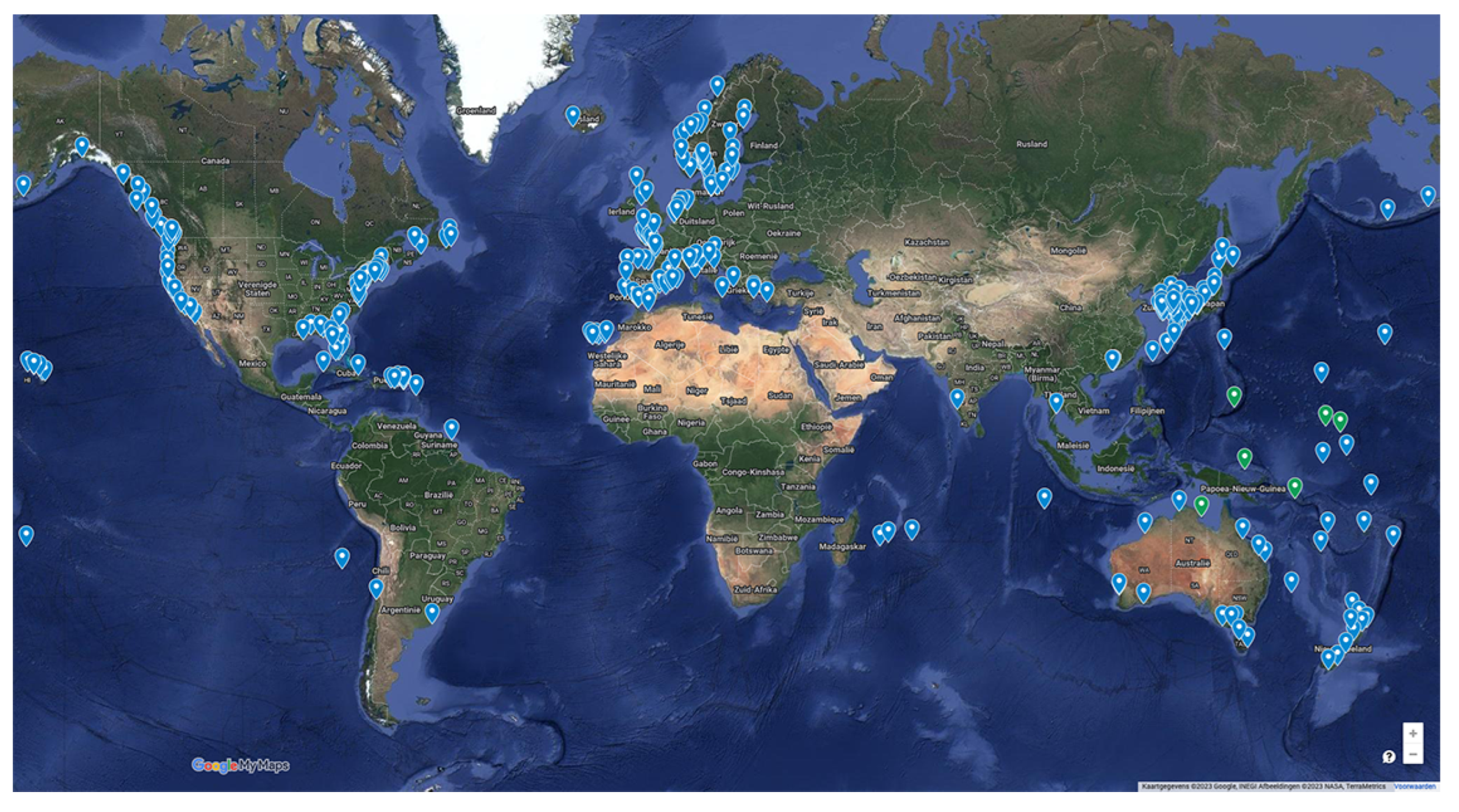
Figure 20 provides the map with the 309 locations of the selected set of tide gauges (light-blue place markers). Ahead of the actual results, the light-green place markers indicate the best six solutions on the basis of correlation.
For GOP CryoSat-2, this statistical analysis resulted in a mean correlation of R = 0.82, a mean standard deviation of
5.7 cm, and mean tilt of the CG−TG difference of 0.17 mm/yr, which nicely fits within the 0.24 mm/yr and −0.10 mm/yr drift values with respect to Jason-2 and Jason-3 found before in
Section 3.1. Basically, we can already draw the conclusion that the CryoSat-2 GOP Baseline-C product is extremely stable (note that we analyze the difference between tide gauge and altimetric sea level, so any ’natural’ sea level rise would be seen by both and cancel out). It is hard to tell exactly where a remaining rate between the tide gauges and altimetric sea level could come from, but it could of course be (partly) due to local vertical land motion. On top of that, one has to realize that the averaged global MSL rate has a ±0.4 mm/yr uncertainty [
41].
For the reference missions REF, we found a mean correlation of R = 0.84, a mean standard deviation of
= 4.9 cm, and a mean tilt of the difference of −0.11 mm/yr (REF−TG).
Table 5 summarizes the results. The average difference in common bias removed (CG−REF) amounts to
cm, which is not the same value as we found as the range bias in
Section 3.1; remember that the crossover analysis is global and covers many more data points, whereas our tide gauge stations are sparse and not evenly distributed but rather close to land and islands, so the average common bias is not a global average and cannot be used as a ‘range bias’.
In
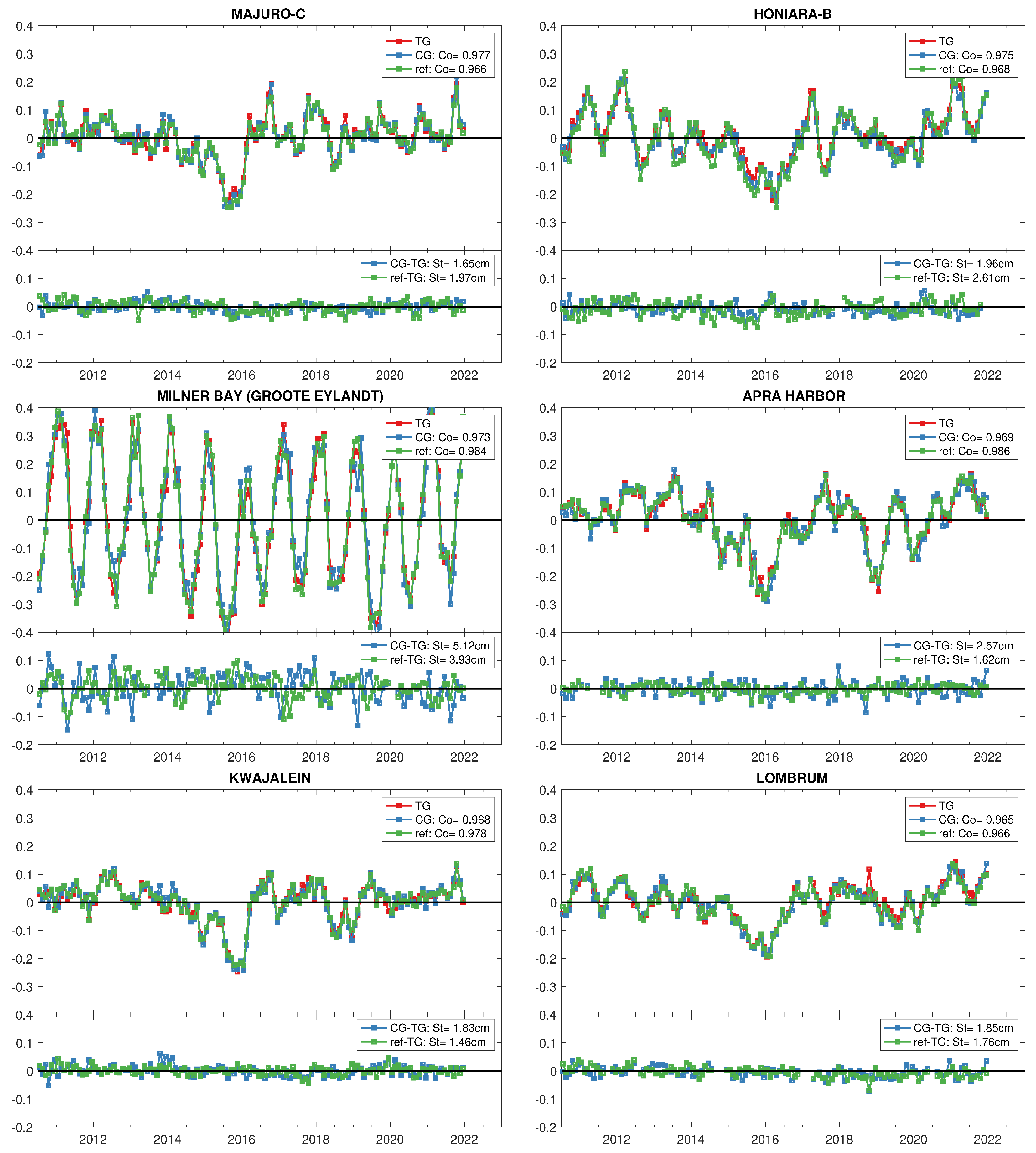
Figure 21, we plotted the six best GOP CryoSat-2 and Jason-2/Jason-3 (REF) tide gauge comparisons (light-green place markers in
Figure 20). The individual statistics for the 309 tide gauges can be found in
Table S1 of the Supplementary Materials. Checking in detail the differences in how both GOP CryoSat-2 and Jason-2/Jason-3 follow the tide gauge data, we conclude that Jason-2/Jason-3 outperforms the CrySat-2 GOP Baseline-C product, as expected, because of REF’s better temporal resolution (10-day repeat cycles vs. 30-day drifting cycles), but that the differences are so small that GOP can be classified to be on par with the reference missions.
3.3.1. Drift after 2022
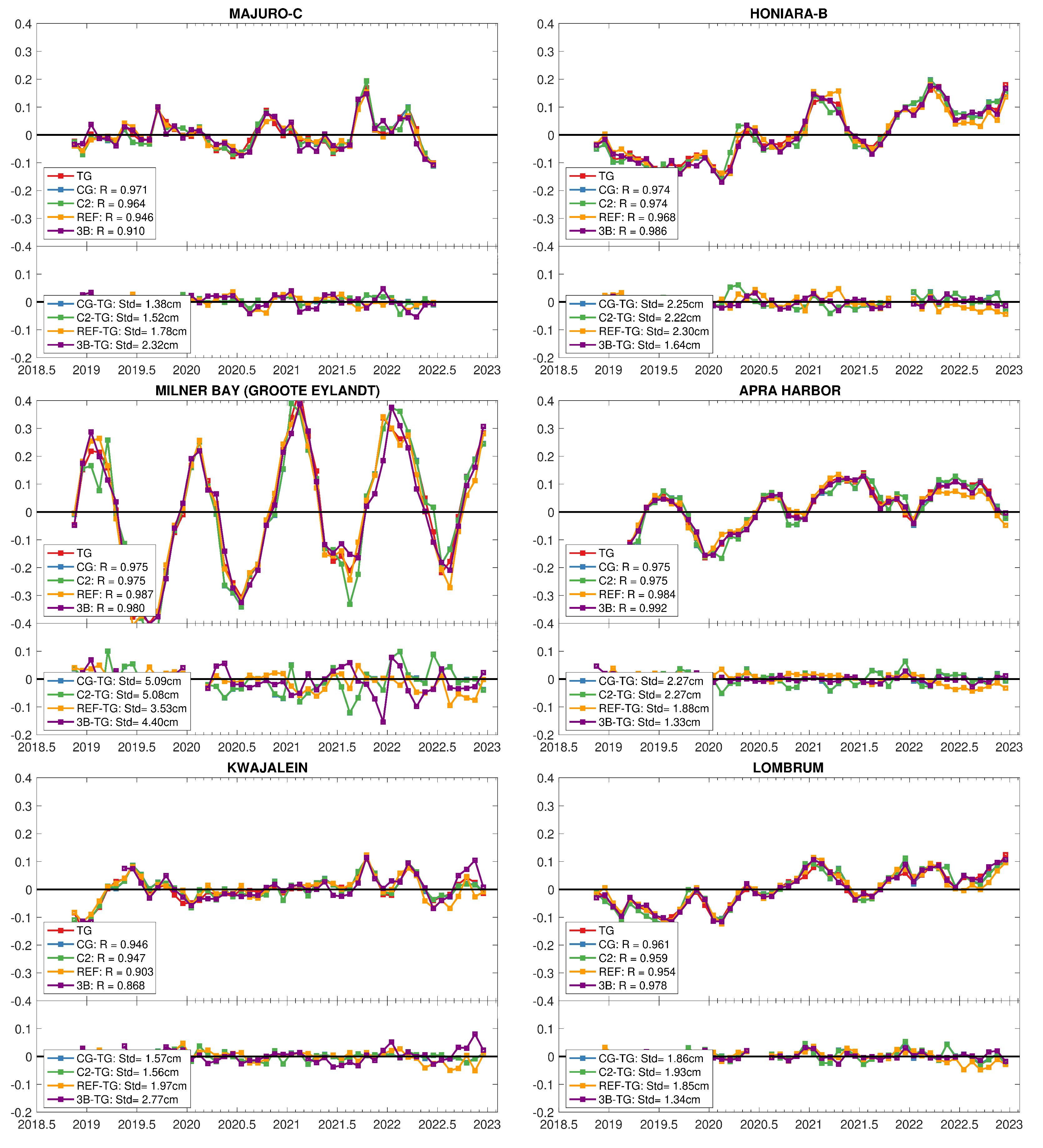
In order to be able to conclude whether the CryoSat-2 GOP data are drifting away from the reference, as was suggested in
Section 3.1 on the basis of a drifting GOP with respect to Sentinel-3A and Sentinel-3B, we extended the tide gauge comparison beyond 2021 (up to 2023) for our six best solutions. The results are given in
Figure 22. Next to the CryoSat-2 GOP (CG) comparison with the tide gauges, we also added the tide gauge comparison with CryoSat-2 RADS (C2), with the sequence of Jason-2, Jason-3, and Sentinel-6A (REF), as well as with Sentinel-3B (3B). The reference mission (REF) was previously defined as the sequence Jason-2–Jason-3, but it has been extended with Sentinel-6A (all following the original TOPEX cycles). For this, we applied a −1.1 cm bias, which was found with the ’help’ of GOP CryoSat-2, as discussed previously in
Section 3.1. Clearly, in
Figure 22, we find no evidence for GOP drifting away from the tide gauges, nor for RADS CryoSat-2, nor for REF. Oppositely, this is also not obvious from the Sentinel-3B result. It is stressed, however, that, in our tide gauges comparison, we are looking at the cm level, whereas in the plot of the time evolution of SLA range bias (
Figure 10), we are looking at the mm level. Meanwhile, referring back to
Section 3.1, we found the cause for the alleged deterioration of GOP with respect to Sentinel-3A and Sentinel-3B after 2022, i.e., jumps in the SWH crossover differences in Sentinel-3A and 3B, leading to jumps in the sea state bias and consequently jumps in the sea level anomaly. Suffice it to say that GOP is so stable that it actually can be adopted as a reference to other missions (remember, we used the XO comparison of GOP with respect to Sentinel-6A to adjust the bias of Sentinel-6A to get it perfectly aligned with the Jason-2–Jason-3 sequence). The GOP CryoSat-2 tide gauge comparison falls short a bit though, like the REF result, when we analyze Sentinel-3B: on numerous occasions, the correlation with the tide gauge is better, as the standard deviation std is smaller, apparently making Sentinel-3B better-suited for tide gauge comparisons. When every operational mission is sufficiently calibrated and validated, the combination of concurrent satellites will obviously give the best sea level results, and CryoSat-2 has proven to be a worthy companion in this operational mix.


