


Evaluation of the SAIL Radiative Transfer Model for Simulating Canopy Reflectance of Row Crop Canopies

 ,
,
Abstract
:
1. Introduction
2. Materials and Methods
2.1. Study Site
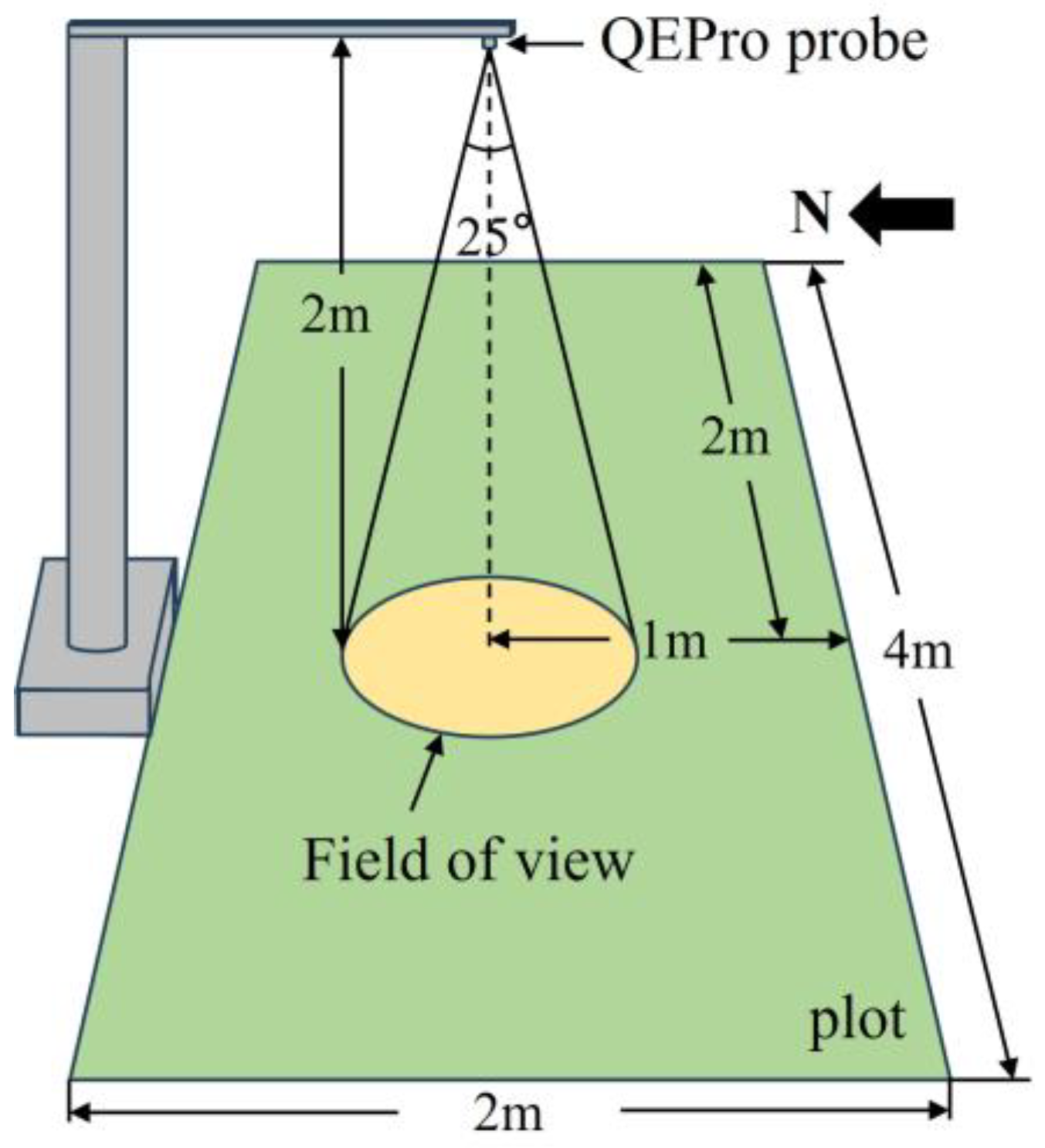
2.2. Field Measurements
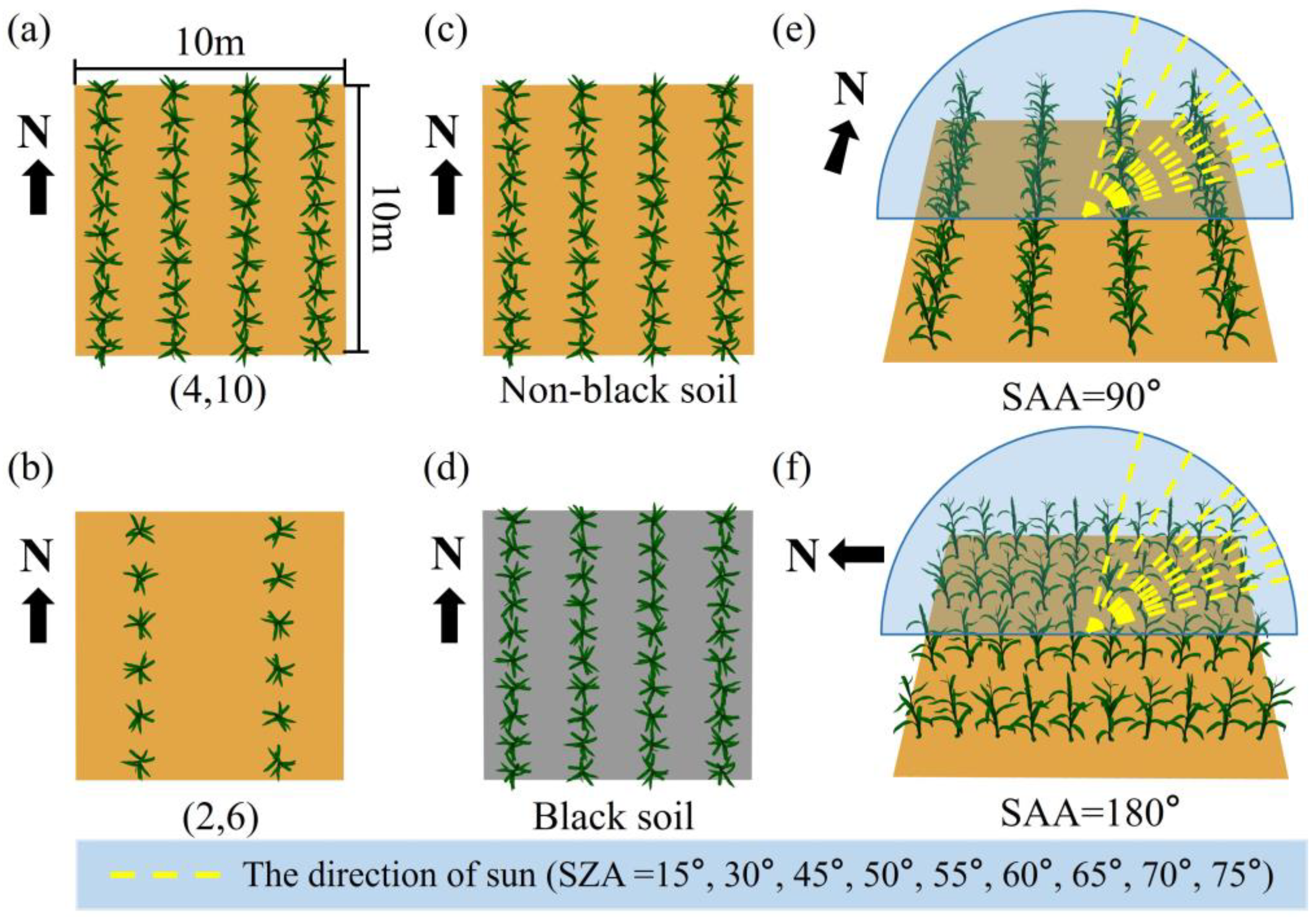
2.3. Synthetic Wheat and Maize Canopies with LESS Model
2.4. SAIL and LESS Model
2.5. Calculating fCover
2.6. Calculating Average Leaf Angle
2.6.1. Estimating Average Leaf Angle of Field Wheat Canopies
2.6.2. Calculating Average Leaf Angle of Synthetic Wheat and Maize Canopies in LESS Model
2.7. Simulating Canopy Reflectance
2.8. Evaluating the Accuracy of SAIL in Modeling the Spectra of Row Canopies
3. Results
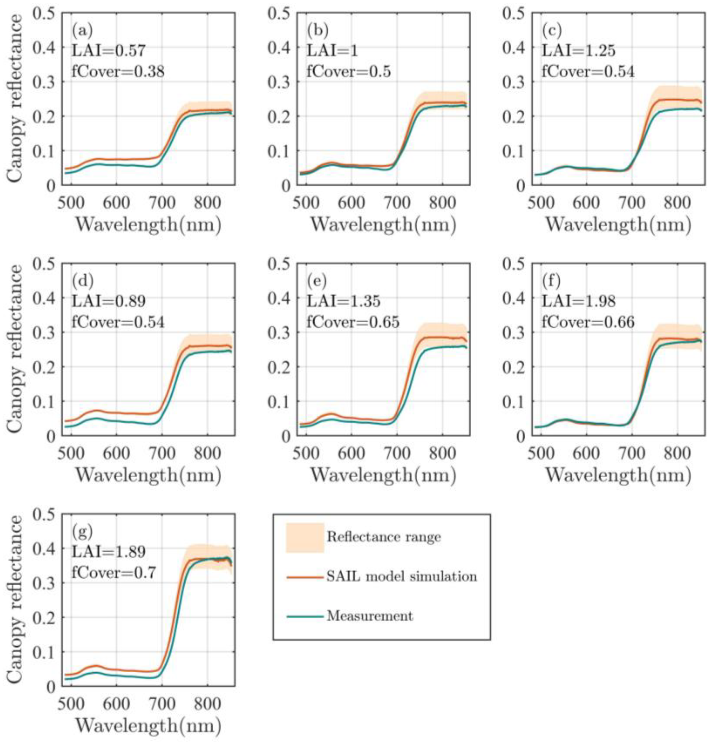
3.1. Evaluation with the Field-Measured Wheat Canopies
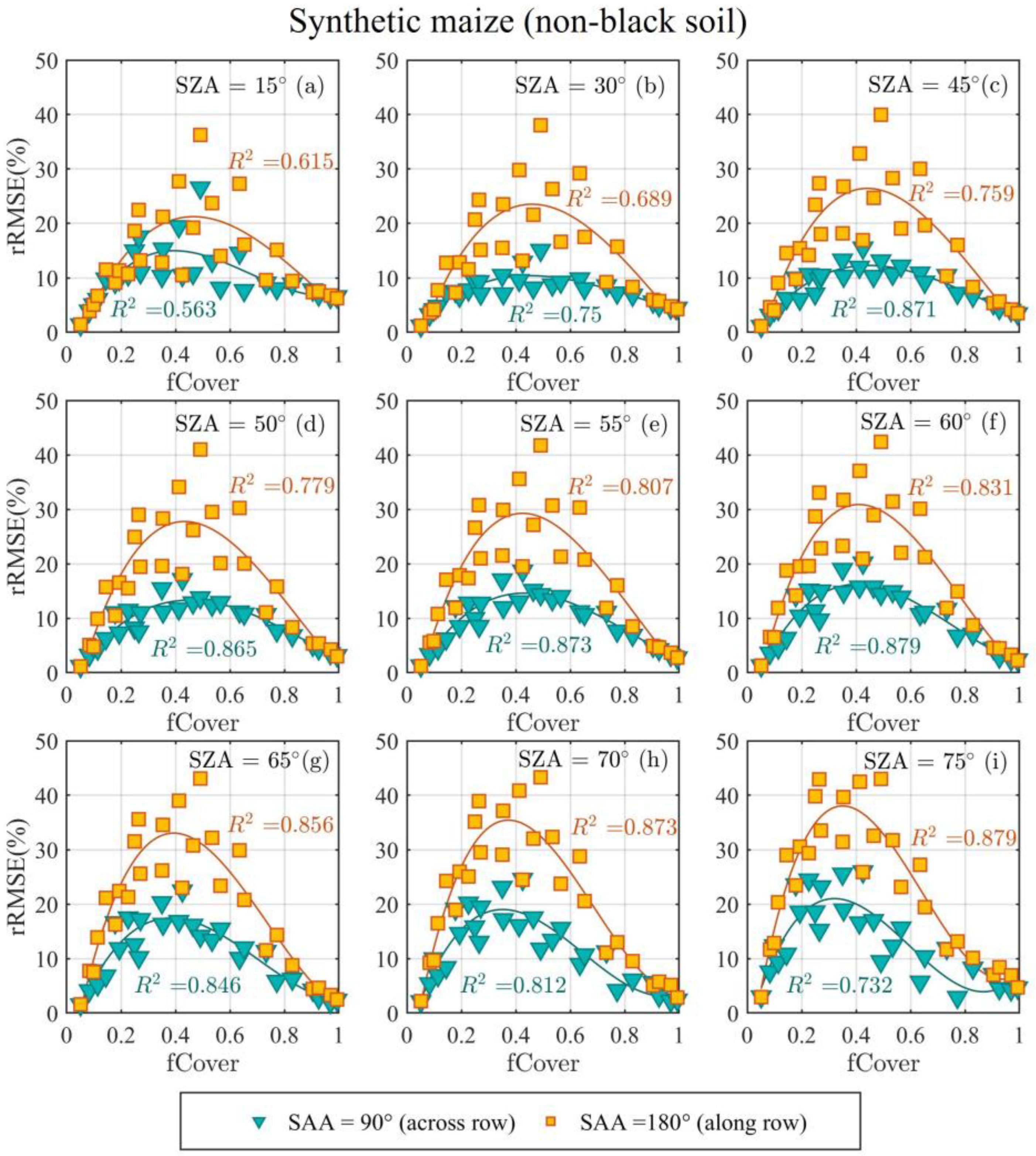
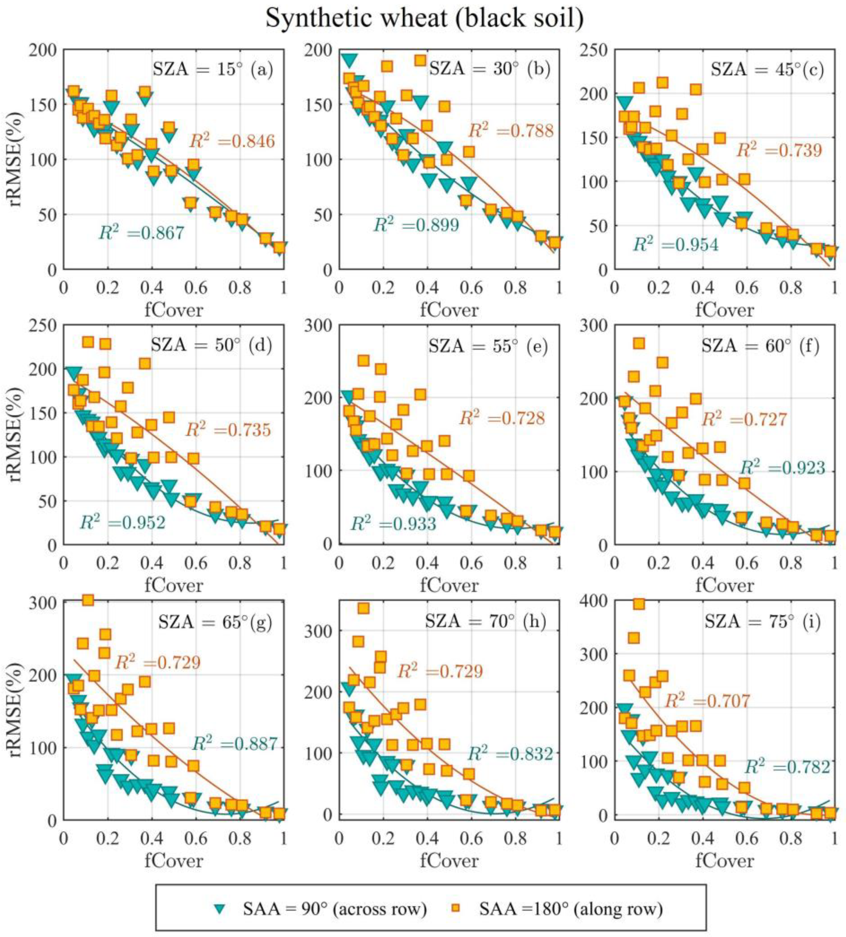
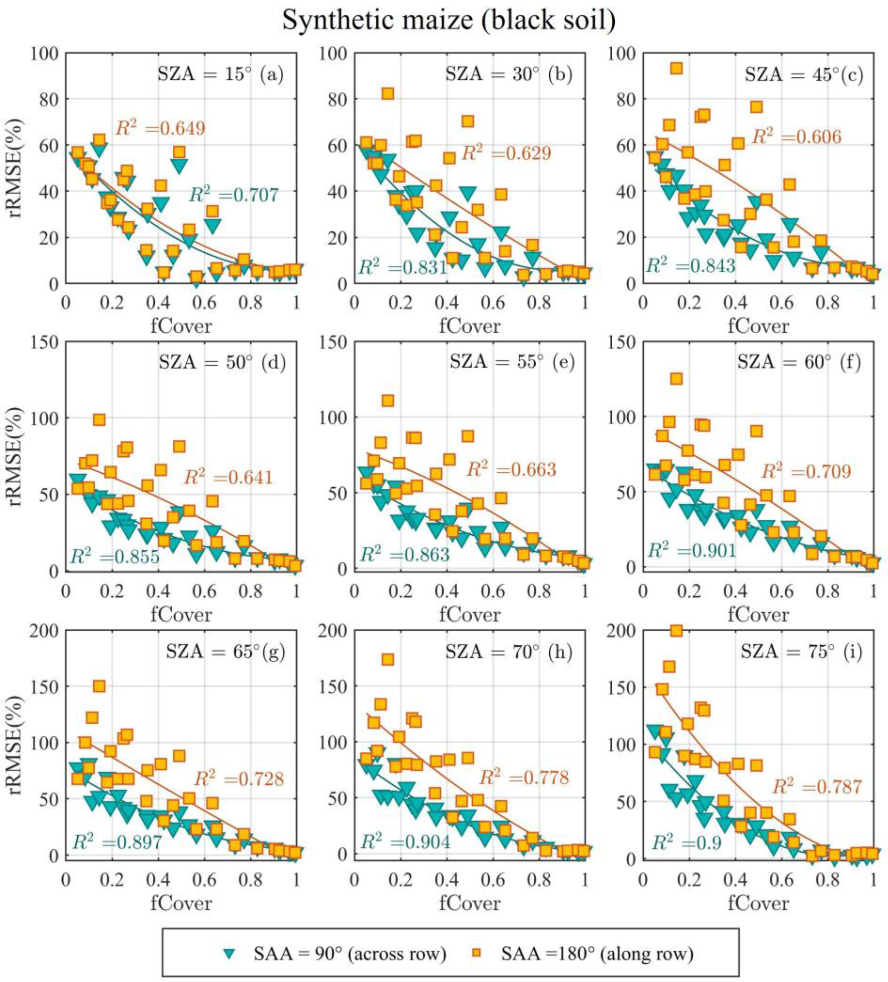
3.2. Evaluation Using the Synthetic Wheat and Maize Canopies
4. Discussion
4.1. Analysis of the Impact Factors on the Accuracy of SAIL in Modeling Row Crop Canopy Reflectance
4.2. The Conditions of Row Canopies Close to Homogeneous Turbid Media
5. Conclusions
Author Contributions
Funding
Data Availability Statement
Conflicts of Interest
References
- Verheof, W. Light Scattering by Leaf Layers with Application to Canopy Reflectance Modeling: The SAIL Model. Remote Sens. Environ. 1984, 16, 125–141. [Google Scholar] [CrossRef]
- Widlowski, J.L.; Taberner, M.; Pinty, B.; Bruniquel-Pinel, V.; Disney, M.; Fernandes, R.; Gastellu-Etchegorry, J.P.; Gobron, N.; Kuusk, A.; Lavergne, T.; et al. Third Radiation Transfer Model Intercomparison (RAMI) Exercise: Documenting Progress in Canopy Reflectance Models. J. Geophys. Res. Atmos. 2007, 112, 1–28. [Google Scholar] [CrossRef]
- Vohland, M.; Mader, S.; Dorigo, W. Applying Different Inversion Techniques to Retrieve Stand Variables of Summer Barley with PROSPECT + SAIL. Int. J. Appl. Earth Obs. Geoinf. 2010, 12, 71–80. [Google Scholar] [CrossRef]
- Kimm, H.; Guan, K.; Jiang, C.; Peng, B.; Gentry, L.F.; Wilkin, S.C.; Wang, S.; Cai, Y.; Bernacchi, C.J.; Peng, J.; et al. Deriving High-Spatiotemporal-Resolution Leaf Area Index for Agroecosystems in the U.S. Corn Belt Using Planet Labs CubeSat and STAIR Fusion Data. Remote Sens. Environ. 2020, 239, 111615. [Google Scholar] [CrossRef]
- Nie, C.; Shi, L.; Li, Z.; Xu, X.; Yin, D.; Li, S.; Jin, X. A Comparison of Methods to Estimate Leaf Area Index Using Either Crop-Specific or Generic Proximal Hyperspectral Datasets. Eur. J. Agron. 2023, 142, 126664. [Google Scholar] [CrossRef]
- Kong, J.; Luo, Z.; Zhang, C.; Tang, M.; Liu, R.; Xie, Z.; Feng, S. Identification of Robust Hybrid Inversion Models on the Crop Fraction of Absorbed Photosynthetically Active Radiation Using PROSAIL Model Simulated and Field Multispectral Data. Agronomy 2023, 13, 2147. [Google Scholar] [CrossRef]
- Singh, P.; Srivastava, P.K.; Verrelst, J.; Mall, R.K.; Pablo, J. Ecological Informatics High Resolution Retrieval of Leaf Chlorophyll Content over Himalayan Pine Forest Using Visible/IR Sensors Mounted on UAV and Radiative Transfer Model. Ecol. Inform. 2023, 75, 102099. [Google Scholar] [CrossRef]
- Badhwar, G.D.; Verhoef, W.; Bunnik, N.J.J. Comparative Study of Suits and Sail Canopy Reflectance Models. Remote Sens. Environ. 1985, 17, 179–195. [Google Scholar] [CrossRef]
- Moulin, S.; Fischer, A.; Dedieu, G.; Delécolle, R. Temporal Variations in Satellite Reflectances at Field and Regional Scales Compared with Values Simulated by Linking Crop Growth and SAIL Models. Remote Sens. Environ. 1995, 54, 261–272. [Google Scholar] [CrossRef]
- Ma, X.; Lu, L.; Ding, J.; Zhang, F.; He, B. Estimating Fractional Vegetation Cover of Row Crops from High Spatial Resolution Image. Remote Sens. 2021, 13, 3874. [Google Scholar] [CrossRef]
- Russell, M. Monitoring Regional Vegetation Change Using Reflectance Measurements from Multiple Solar Zenith Angles. Environ. Int. 2001, 27, 211–217. [Google Scholar] [CrossRef]
- Zhao, F.; Gu, X.; Verhoef, W.; Wang, Q.; Yu, T.; Liu, Q.; Huang, H.; Qin, W.; Chen, L.; Zhao, H. A Spectral Directional Reflectance Model of Row Crops. Remote Sens. Environ. 2010, 114, 265–285. [Google Scholar] [CrossRef]
- Jafarbiglu, H.; Pourreza, A. Impact of Sun-View Geometry on Canopy Spectral Reflectance Variability. ISPRS J. Photogramm. Remote Sens. 2023, 196, 270–286. [Google Scholar] [CrossRef]
- Major, D.J.; Schaalje, G.B.; Wiegand, C.; Blad, B.L. Accuracy and Sensitivity Analyses of SAIL Model-Predicted Reflectance of Maize. Remote Sens. Environ. 1992, 41, 61–70. [Google Scholar] [CrossRef]
- Duke, C.; Guérif, M. Crop Reflectance Estimate Errors from the SAIL Model Due to Spatial and Temporal Variability of Canopy and Soil Characteristics. Remote Sens. Environ. 1998, 66, 286–297. [Google Scholar] [CrossRef]
- Li, D.; Chen, J.M.; Zhang, X.; Yan, Y.; Zhu, J.; Zheng, H.; Zhou, K.; Yao, X.; Tian, Y.; Zhu, Y.; et al. Improved Estimation of Leaf Chlorophyll Content of Row Crops from Canopy Reflectance Spectra through Minimizing Canopy Structural Effects and Optimizing Off-Noon Observation Time. Remote Sens. Environ. 2020, 248, 111985. [Google Scholar] [CrossRef]
- Yang, P. Exploring the Interrelated Effects of Soil Background, Canopy Structure and Sun-Observer Geometry on Canopy Photochemical Reflectance Index. Remote Sens. Environ. 2022, 279, 113133. [Google Scholar] [CrossRef]
- Goel, N.S.; Grier, T. Estimation of Canopy Parameters for Inhomogeneous Vegetation Canopies from Reflectance Data i. Two-Dimensional Row Canopy. Int. J. Remote Sens. 1986, 7, 665–681. [Google Scholar] [CrossRef]
- Nilson, T.; Kuusk, A. A Reflectance Model for the Homogeneous Plant Canopy and Its Inversion. Remote Sens. Environ. 1989, 27, 157–167. [Google Scholar] [CrossRef]
- Zhou, K.; Guo, Y.; Geng, Y.; Zhu, Y.; Cao, W.; Tian, Y. Development of a Novel Bidirectional Canopy Reflectance Model for Row-Planted Rice and Wheat. Remote Sens. 2014, 6, 7632–7659. [Google Scholar] [CrossRef]
- Ma, X.; Wang, T.; Lu, L. A Refined Four-Stream Radiative Transfer Model for Row-Planted Crops. Remote Sens. 2020, 12, 1290. [Google Scholar] [CrossRef]
- Zhang, T.; Ren, H.; Sun, Y.; Zhang, C.; Qin, Q. Simultaneous Retrieval Of Leaf Area Index And Fractional Canopy Cover Using SAIL Model And PSO Algorithm. In Proceedings of the 2017 IEEE International Geoscience and Remote Sensing Symposium (IGARSS), Fort Worth, TX, USA, 23–28 July 2017; pp. 5446–5449. [Google Scholar] [CrossRef]
- Liu, K.; Zhou, Q.B.; Wu, W.B.; Xia, T.; Tang, H.J. Estimating the Crop Leaf Area Index Using Hyperspectral Remote Sensing. J. Integr. Agric. 2016, 15, 475–491. [Google Scholar] [CrossRef]
- Zhang, P.; Zhao, F.; Guo, Y.; Zhao, H.; Zhao, Y.; Dong, L. Sensitivity Analysis of the Row Model’s Input Parameters. In Proceedings of the 2014 The Third International Conference on Agro-Geoinformatics, Beijing, China, 11–14 August 2014; pp. 1–5. [Google Scholar] [CrossRef]
- Wan, L.; Zhang, J.; Dong, X.; Du, X.; Zhu, J.; Sun, D. Unmanned Aerial Vehicle-Based Field Phenotyping of Crop Biomass Using Growth Traits Retrieved from PROSAIL Model. Comput. Electron. Agric. 2021, 187, 106304. [Google Scholar] [CrossRef]
- Li, L.; Mu, X.; Jiang, H.; Chianucci, F.; Hu, R.; Song, W.; Qi, J.; Liu, S.; Zhou, J.; Chen, L.; et al. Review of Ground and Aerial Methods for Vegetation Cover Fraction (FCover) and Related Quantities Estimation: Definitions, Advances, Challenges, and Future Perspectives. ISPRS J. Photogramm. Remote Sens. 2023, 199, 133–156. [Google Scholar] [CrossRef]
- Kollenkark, J.C.; Vanderbilt, V.C.; Daughtry, C.S.T.; Bauer, M.E. Influence of Solar Illumination Angle on Soybean Canopy Reflectance. Appl. Opt. 1982, 21, 1179. [Google Scholar] [CrossRef]
- Roujean, J.L.; Breon, F.M. Estimating PAR Absorbed by Vegetation from Bidirectional Reflectance Measurements. Remote Sens. Environ. 1995, 51, 375–384. [Google Scholar] [CrossRef]
- Yu, K.; Lenz-Wiedemann, V.; Chen, X.; Bareth, G. Estimating Leaf Chlorophyll of Barley at Different Growth Stages Using Spectral Indices to Reduce Soil Background and Canopy Structure Effects. ISPRS J. Photogramm. Remote Sens. 2014, 97, 58–77. [Google Scholar] [CrossRef]
- Jiang, H.; Wei, X.; Chen, Z.; Zhu, M.; Yao, Y.; Zhang, X.; Jia, K. Influence of Different Soil Reflectance Schemes on the Retrieval of Vegetation LAI and FVC from PROSAIL in Agriculture Region. Comput. Electron. Agric. 2023, 212, 108165. [Google Scholar] [CrossRef]
- Goel, N.S. Models of Vegetation Canopy Reflectance and Their Use in Estimation of Biophysical Parameters from Reflectance Data. Remote Sens. Rev. 1988, 4, 1–212. [Google Scholar] [CrossRef]
- Van Wittenberghe, S.; Alonso, L.; Verrelst, J.; Moreno, J.; Samson, R. Bidirectional Sun-Induced Chlorophyll Fluorescence Emission Is Influenced by Leaf Structure and Light Scattering Properties—A Bottom-up Approach. Remote Sens. Environ. 2015, 158, 169–179. [Google Scholar] [CrossRef]
- Suits, G.H. Extension of a Uniform Canopy Reflectance Model to Include Row Effects. Remote Sens. Environ. 1983, 13, 113–129. [Google Scholar] [CrossRef]
- Andrieu, B.; Baret, F.; Jacquemoud, S.; Malthus, T.; Steven, M. Evaluation of an Improved Version of SAIL Model for Simulating Bidirectional Reflectance of Sugar Beet Canopies. Remote Sens. Environ. 1997, 60, 247–257. [Google Scholar] [CrossRef]
- Jacquemoud, S.; Baret, F. PROSPECT: A Model of Leaf Optical Properties Spectra. Remote Sens. Environ. 1990, 34, 75–91. [Google Scholar] [CrossRef]
- Jacquemoud, S.; Verhoef, W.; Baret, F.; Bacour, C.; Zarco-Tejada, P.J.; Asner, G.P.; François, C.; Ustin, S.L. PROSPECT + SAIL Models: A Review of Use for Vegetation Characterization. Remote Sens. Environ. 2009, 113, S56–S66. [Google Scholar] [CrossRef]
- Verhoef, W.; Jia, L.; Xiao, Q.; Su, Z. Unified Optical-Thermal Four-Stream Radiative Transfer Theory for Homogeneous Vegetation Canopies. IEEE Trans. Geosci. Remote Sens. 2007, 45, 1808–1822. [Google Scholar] [CrossRef]
- Qi, J.; Xie, D.; Yin, T.; Yan, G.; Gastellu-Etchegorry, J.P.; Li, L.; Zhang, W.; Mu, X.; Norford, L.K. LESS: LargE-Scale Remote Sensing Data and Image Simulation Framework over Heterogeneous 3D Scenes. Remote Sens. Environ. 2019, 221, 695–706. [Google Scholar] [CrossRef]
- Gitelson, A.A.; Kaufman, Y.J.; Stark, R.; Rundquist, D. Novel Algorithms for Remote Estimation of Vegetation Fraction. Remote Sens. Environ. 2002, 80, 76–87. [Google Scholar] [CrossRef]
- Verhoef, W. Theory of Radiative Transfer Models Applied in Optical Remote Sensing of Vegetation Canopies. Ph.D. Thesis, Wageningen University, Wageningen, The Netherlands, 1998. [Google Scholar]
- Wang, W.M.; Li, Z.L.; Su, H.B. Comparison of Leaf Angle Distribution Functions: Effects on Extinction Coefficient and Fraction of Sunlit Foliage. Agric. For. Meteorol. 2007, 143, 106–122. [Google Scholar] [CrossRef]
- Yang, P.; van der Tol, C.; Verhoef, W.; Damm, A.; Schickling, A.; Kraska, T.; Muller, O.; Rascher, U. Using Reflectance to Explain Vegetation Biochemical and Structural Effects on Sun-Induced Chlorophyll Fluorescence. Remote Sens. Environ. 2019, 231, 110996. [Google Scholar] [CrossRef]
- Zou, X.; Mõttus, M.; Tammeorg, P.; Torres, C.L.; Takala, T.; Pisek, J.; Mäkelä, P.; Stoddard, F.L.; Pellikka, P. Photographic Measurement of Leaf Angles in Field Crops. Agric. For. Meteorol. 2014, 184, 137–146. [Google Scholar] [CrossRef]
- Huang, W.; Niu, Z.; Wang, J.; Liu, L.; Zhao, C.; Liu, Q. Identifying Crop Leaf Angle Distribution Based on Two-Temporal and Bidirectional Canopy Reflectance. IEEE Trans. Geosci. Remote Sens. 2006, 44, 3601–3608. [Google Scholar] [CrossRef]
- Huete, A.R.; Jackson, R.D.; Post, D.F. Spectral Response of a Plant Canopy with Different Soil Backgrounds. Remote Sens. Environ. 1985, 17, 37–53. [Google Scholar] [CrossRef]
- Ryu, Y.; Verfaillie, J.; Macfarlane, C.; Kobayashi, H.; Sonnentag, O.; Vargas, R.; Ma, S.; Baldocchi, D.D. Continuous Observation of Tree Leaf Area Index at Ecosystem Scale Using Upward-Pointing Digital Cameras. Remote Sens. Environ. 2012, 126, 116–125. [Google Scholar] [CrossRef]
- Macfarlane, C.; Hoffman, M.; Eamus, D.; Kerp, N.; Higginson, S.; Mcmurtrie, R.; Adams, M. Estimation of Leaf Area Index in Eucalypt Forest Using Digital Photography. Agric. For. Meteorol. 2007, 143, 176–188. [Google Scholar] [CrossRef]


| Wheat Plot | LAI | fCover |
|---|---|---|
| (a) | 0.57 | 0.38 |
| (b) | 1.00 | 0.50 |
| (c) | 1.25 | 0.54 |
| (d) | 0.89 | 0.54 |
| (e) | 1.35 | 0.65 |
| (f) | 1.98 | 0.66 |
| (g) | 1.89 | 0.70 |
| Configuration of Row (Wheat|Maize) | LAI (Wheat|Maize) | fCover (Wheat|Maize) | Configuration of Row (Wheat|Maize) | LAI (Wheat|Maize) | fCover (Wheat|Maize) |
|---|---|---|---|---|---|
| (4,4)|(2,2) | 0.08|0.05 | 0.046|0.051 | (20,20)|(10,10) | 1.94|1.19 | 0.292|0.425 |
| (4,12)|(2,6) | 0.23|0.14 | 0.066|0.083 | (16,30)|(8,15) | 2.32|1.42 | 0.334|0.464 |
| (8,8)|(4,4) | 0.31|0.19 | 0.077|0.099 | (12,60)|(6,30) | 3.46|2.13 | 0.369|0.491 |
| (4,20)|(2,10) | 0.39|0.24 | 0.087|0.114 | (16,40)|(8,20) | 3.09|1.89 | 0.398|0.534 |
| (4,30)|(2,15) | 0.58|0.35 | 0.110|0.144 | (20,30)|(10,15) | 2.90|1.77 | 0.408|0.565 |
| (12,12)|(6,6) | 0.70|0.43 | 0.128|0.178 | (16,60)|(8,30) | 4.62|2.84 | 0.478|0.635 |
| (8,20)|(4,10) | 0.77|0.48 | 0.138|0.193 | (20,40)|(10,20) | 3.86|2.36 | 0.489|0.652 |
| (12,16)|(6,8) | 0.93|0.57 | 0.159|0.226 | (30,30)|(15,15) | 4.35|2.64 | 0.576|0.733 |
| (8,30)|(4,15) | 1.16|0.71 | 0.185|0.249 | (20,60)|(10,30) | 5.77|3.55 | 0.589|0.772 |
| (8,40)|(4,20) | 1.55|0.86 | 0.217|0.265 | (30,40)|(15,20) | 5.79|3.51 | 0.688|0.829 |
| (12,20)|(6,10) | 1.16|0.71 | 0.189|0.271 | (40,40)|(20,20) | 7.71|4.69 | 0.808|0.904 |
| (16,20)|(8,10) | 1.55|0.95 | 0.241|0.350 | (30,50)|(15,30) | 7.23|5.28 | 0.761|0.926 |
| (12,30)|(6,15) | 1.74|1.06 | 0.259|0.354 | (40,60)|(20,30) | 11.51|7.04 | 0.916|0.969 |
| (12,40)|(6,20) | 2.32|1.42 | 0.306|0.412 | (60,60)|(30,30) | 17.21|10.58 | 0.979|0.993 |
| Parameter | Interpretation | Field (Wheat) | Synthetic (Wheat and Maize) |
|---|---|---|---|
| Leaf reflectance | Average measurement | Default (Mean reflectance = 0.22) | |
| Leaf transmittance | Average measurement | Default (Mean reflectance = 0.25) | |
| ALA | Average leaf angle | 53.5° (range from 40° to 60° for potential uncertainty) | Wheat: 70.46° Maize: 55.36° |
| LAI | Leaf area index | Average measurement | Calculated |
| Soil reflectance | Measurement | Default (Mean reflectance = 0.4) | |
| Solar zenith angle | Calculated from latitude, longitude and date time | 15°, 30°, 45°, 50°, 55°, 60°, 65°, 70°, 75° | |
| Observe zenith angle | 0° | 0° | |
| The azimuth angle between sun and observed direction | Arbitrary | Arbitrary | |
| Hotspot parameter | 0.01 | 0.01 |
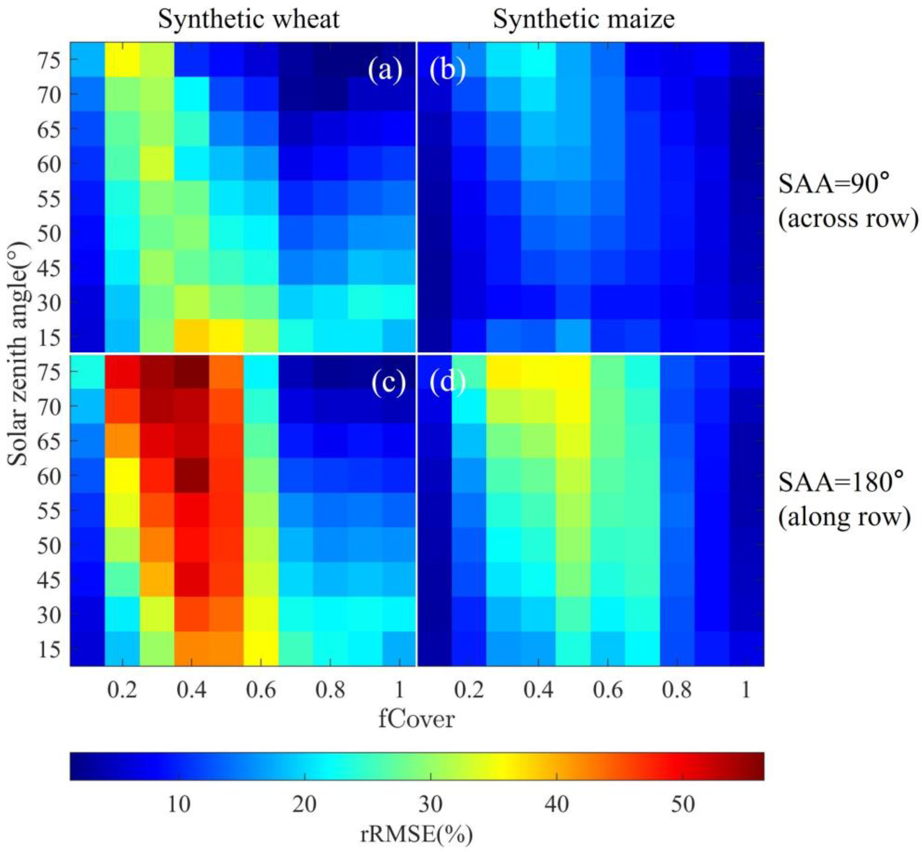
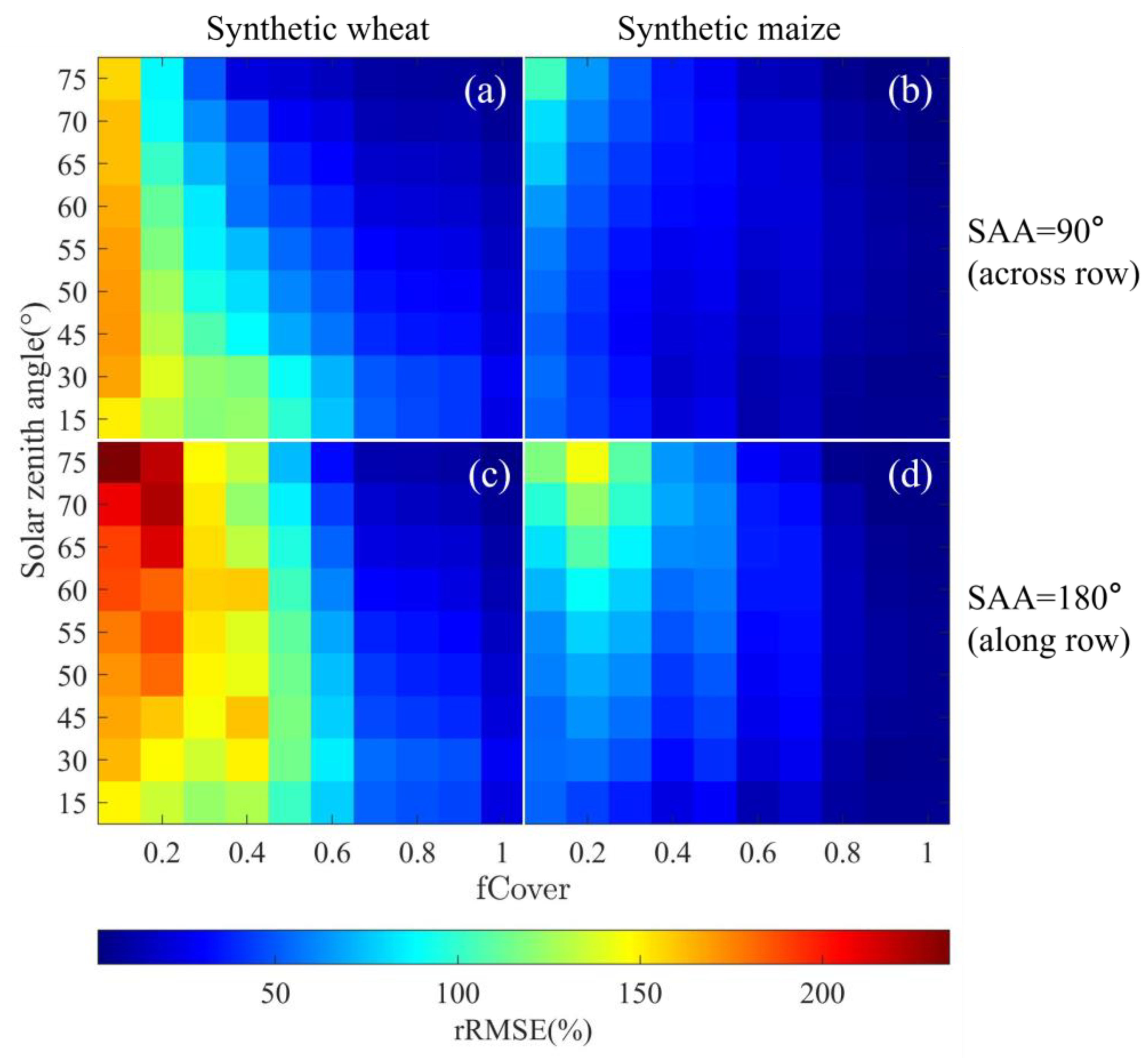
| SZA (°) | SAA (°) | Synthetic Wheat | Synthetic Maize | ||
|---|---|---|---|---|---|
| Mean rRMSE (%) | Difference (%) | Mean rRMSE (%) | Difference (%) | ||
| 15 | 90 | 24.1 | 1.9 | 10.3 | 3.4 |
| 180 | 26 | 13.8 | |||
| 30 | 90 | 22.5 | 5.3 | 7.5 | 7 |
| 180 | 27.9 | 14.5 | |||
| 45 | 90 | 21.3 | 9.2 | 8.3 | 7.8 |
| 180 | 30.5 | 16.1 | |||
| 50 | 90 | 20.9 | 10.5 | 8.8 | 8.1 |
| 180 | 31.3 | 16.9 | |||
| 55 | 90 | 20.4 | 11.9 | 9.5 | 8.2 |
| 180 | 32.4 | 17.8 | |||
| 60 | 90 | 19.8 | 13.4 | 10.2 | 8.4 |
| 180 | 33.2 | 18.7 | |||
| 65 | 90 | 19.2 | 15.1 | 10.8 | 9.0 |
| 180 | 34.3 | 19.9 | |||
| 70 | 90 | 18.5 | 16.9 | 11.7 | 9.7 |
| 180 | 35.4 | 21.4 | |||
| 75 | 90 | 18 | 18.7 | 13.1 | 10.2 |
| 180 | 36.7 | 23.4 | |||
| SZA (°) | SAA (°) | Synthetic Wheat | Synthetic Maize | ||
|---|---|---|---|---|---|
| Mean rRMSE (%) | Difference (%) | Mean rRMSE (%) | Difference (%) | ||
| 15 | 90 | 106.8 | 2.8 | 25.5 | 1.6 |
| 180 | 109.6 | 27 | |||
| 30 | 90 | 109.8 | 11.7 | 24.6 | 9.2 |
| 180 | 121.5 | 33.8 | |||
| 45 | 90 | 96.9 | 29.1 | 24.2 | 14 |
| 180 | 126.0 | 38.2 | |||
| 50 | 90 | 91.4 | 36.6 | 26.5 | 15.4 |
| 180 | 128.0 | 41.9 | |||
| 55 | 90 | 85.0 | 44.1 | 28.5 | 17.5 |
| 180 | 129.1 | 45.9 | |||
| 60 | 90 | 78.3 | 52.3 | 31.3 | 19.5 |
| 180 | 130.6 | 50.8 | |||
| 65 | 90 | 71.8 | 59 | 33.7 | 22.7 |
| 180 | 130.9 | 56.4 | |||
| 70 | 90 | 64.5 | 66.9 | 35 | 27.1 |
| 180 | 131.3 | 62.1 | |||
| 75 | 90 | 56.1 | 76.2 | 37 | 29.4 |
| 180 | 132.2 | 66.4 | |||
Disclaimer/Publisher’s Note: The statements, opinions and data contained in all publications are solely those of the individual author(s) and contributor(s) and not of MDPI and/or the editor(s). MDPI and/or the editor(s) disclaim responsibility for any injury to people or property resulting from any ideas, methods, instructions or products referred to in the content. |
© 2023 by the authors. Licensee MDPI, Basel, Switzerland. This article is an open access article distributed under the terms and conditions of the Creative Commons Attribution (CC BY) license (https://creativecommons.org/licenses/by/4.0/).
Share and Cite
Han, D.; Liu, J.; Zhang, R.; Liu, Z.; Guo, T.; Jiang, H.; Wang, J.; Zhao, H.; Ren, S.; Yang, P. Evaluation of the SAIL Radiative Transfer Model for Simulating Canopy Reflectance of Row Crop Canopies. Remote Sens. 2023, 15, 5433. https://doi.org/10.3390/rs15235433
Han D, Liu J, Zhang R, Liu Z, Guo T, Jiang H, Wang J, Zhao H, Ren S, Yang P. Evaluation of the SAIL Radiative Transfer Model for Simulating Canopy Reflectance of Row Crop Canopies. Remote Sensing. 2023; 15(23):5433. https://doi.org/10.3390/rs15235433
Chicago/Turabian StyleHan, Dalei, Jing Liu, Runfei Zhang, Zhigang Liu, Tingrui Guo, Hao Jiang, Jin Wang, Huarong Zhao, Sanxue Ren, and Peiqi Yang. 2023. "Evaluation of the SAIL Radiative Transfer Model for Simulating Canopy Reflectance of Row Crop Canopies" Remote Sensing 15, no. 23: 5433. https://doi.org/10.3390/rs15235433
APA StyleHan, D., Liu, J., Zhang, R., Liu, Z., Guo, T., Jiang, H., Wang, J., Zhao, H., Ren, S., & Yang, P. (2023). Evaluation of the SAIL Radiative Transfer Model for Simulating Canopy Reflectance of Row Crop Canopies. Remote Sensing, 15(23), 5433. https://doi.org/10.3390/rs15235433