Abstract
Due to the complex range migration characteristics of large squint angle synthetic aperture radar (SAR), it is difficult for traditional SAR deceptive jamming algorithms to balance focusing ability and computational efficiency. There is an urgent demand for proposing a deceptive jamming algorithm against large squint angle SAR in the field of SAR jamming. This article proposes a deceptive jamming algorithm against SAR with large squint angles based on non-linear chirp scaling and low azimuth sampling reconstruction (NLCSR). The NLCSR algorithm uses a high-order approximation of a high-precision model to accurately construct the jammer’s frequency response (JFR) function. In line with the notion of low azimuth sampling processing of the transformation domain, the construction of the space-variant azimuth modulation phase item is completed using the non-linear chirp scaling method. Compared with the traditional deceptive jamming algorithms against the large squint angle SAR, the NLCSR algorithm only needs Fourier transform and complex multiplication while ensuring the focusing ability, which is easier to implement on an efficient parallel digital signal processor based on fast Fourier transform (FFT). Simulation results prove the superior property of the NLCSR algorithm in focusing ability and computational efficiency. Compared to the existing large squint angle SAR deceptive jamming algorithm, the focusing ability of the NLCSR algorithm is almost the same, and the calculation efficiency is improved by at least 52.1%.
1. Introduction
Synthetic aperture radar (SAR) is a high-resolution microwave imaging system with all-day availability, all-weather capability, substantial processing gain, and robust anti-jamming capabilities [1]. Nevertheless, its application in the military raises concerns about the vulnerability of intelligence security. Consequently, electronic countermeasures technology (ECM) designed to counter SAR has experienced rapid development [2,3,4,5]. The low power consumption and high fidelity advantages of SAR deceptive jamming have garnered significant attention [6,7,8,9,10,11,12,13,14,15,16,17,18,19,20,21,22].
1.1. Background
At present, SAR deceptive jamming mainly relies on the modulation retransmission mechanism [23,24]. The SAR deceptive jammer generates a jammer’s frequency response (JFR) function at each pulse repetition interval (PRI), modulates and forwards the intercepted pulse, and then completes SAR deceptive jamming. Therefore, generating the JFR is the key to the research of SAR deceptive jamming. The traditional SAR deceptive JFR generation method requires point-by-point superposition calculation of false electromagnetic features in continuous pulse intervals [7], and the computational burden of jamming modulation is unbearable for jammer.
In order to satisfy the real-time SAR deceptive jamming, many scholars have proposed efficient algorithms to decrease the computational load of the construction of jamming modulation, which can be classified into two distinct categories: azimuth time domain deceptive jamming and azimuth frequency-domain deceptive jamming. The former includes the segmented modulation algorithm [8,9] and the template segmented time-delay frequency-shift algorithm [10], which reduces computational complexity through slant range approximation equations and range-azimuth fractal modulation, and the calculation of the azimuth time domain makes it easier to expand research into various complex scenarios. However, the approximation error of its algorithm is too large, and the integral operation cannot be avoided. Neither the jamming accuracy nor the jamming efficiency can meet the high-resolution real-time jamming requirements. The latter includes the frequency-domain three-stage algorithm [11], the inverse range Doppler algorithm [12], the inverse Omega-K algorithm [13], frequency-domain preprocessing algorithm [14], which requires the construction of cross-coupling terms in the azimuth frequency domain to reduce computational complexity. Jamming modulation does not require integral operations, and the jamming accuracy is relatively high. However, its algorithm relies on interpolation calculations, and jamming modulation efficiency and applicability also face obstacles in actual jamming.
1.2. Problem Statement and Contributions
Most deceptive jamming algorithms rely on low-order approximations of the jamming signal’s cross-coupling term to improve computational efficiency. Such algorithm design can only be applied against SAR systems with slight cross-coupling in the anti-echo, such as side-looking, slight squint angle, and low-resolution SAR [25]. However, with the improvement of SAR observation flexibility and high-resolution observation requirements, SAR systems with large squint angles and high resolution have been widely used. The complex imaging geometry model of SAR with large squint angles will bring severe cross-coupling phenomena and high-azimuth oversampling characteristics. Existing deceptive jamming algorithms cannot construct complex cross-coupling terms with sufficient accuracy, and the large-azimuth oversampling characteristics will also bring excessive computational burden, making it difficult to meet the requirements of SAR deceptive jamming at large squint angles for jamming focusing capabilities and computational efficiency. Liu et al. presented an inverse Omega-K (IK)-based deceptive jamming algorithm [13] that uses Stolt interpolation to construct the high-order coupling phase term in the JFR function, which can complete high-resolution SAR for large squint angle deceptive jamming. However, the Stolt interpolation accuracy of the IK algorithm is prone to the Gibbs phenomenon, and the interpolation operation is inefficient and difficult to apply to high-efficiency parallel digital signal processors [1,26]. Balancing jamming focusing ability and computing efficiency is still challenging for jamming high-resolution SAR with large squint angles.
An efficient large squint SAR deceptive jamming algorithm based on non-linear chirp scaling and low azimuth sampling reconstruction (NLCSR) is proposed in this article. On the one hand, to overcome the high azimuth oversampling and severe cross-coupling characteristics of SAR with large squint angles, the NLCSR algorithm mainly adopts the JFR construction scheme that removes the linear range walk term. In this scheme, the number of azimuth sampling points required for the construction of the JFR can be reduced, and the cross-coupling degree of the JFR can also be reduced. Therefore, the high-order cross-coupling term of the large squint angle SAR signal can be directly constructed by reference slant range. On the other hand, considering the space-variant effect of the azimuth modulation term brought about by removing the range walking term, the non-linear frequency modulation scaling method is used in the azimuth time frequency transformation domain to complete the construction of the space-variant azimuth modulation term. Thus, the construction accuracy of the JFR can be ensured. The NLCSR algorithm merges high-precision approximation of the high-order coupling term with low azimuth sampling transform domain processing efficiency, which can overcome the high-efficiency and high-precision deceptive jamming dilemma for large squint angle SAR.
The article is organized as follows. Section 2 analyzes the basic principle and dilemma of SAR deceptive jamming at a large squint angle and then gives the detailed derivation process of the NLCSR algorithm. In Section 3, the NLCSR algorithm is verified from the simulation of false point targets and actual scene, the validity limit analysis, and computational complexity analysis. Section 4 discusses the NLCSR algorithm according to the effectiveness analysis and experimental results. Finally, Section 5 provides concluding remarks for this article.
2. Deceptive Jamming Algorithm Based on Non-Linear Chirp Scaling and Low Azimuth Sampling Reconstruction
In this section, the squint observation model of the SAR system and deceptive jamming model are introduced initially. Subsequently, a detailed derivation of the NLCSR algorithm’s theory is provided.
2.1. Squint Angle SAR Signal Model
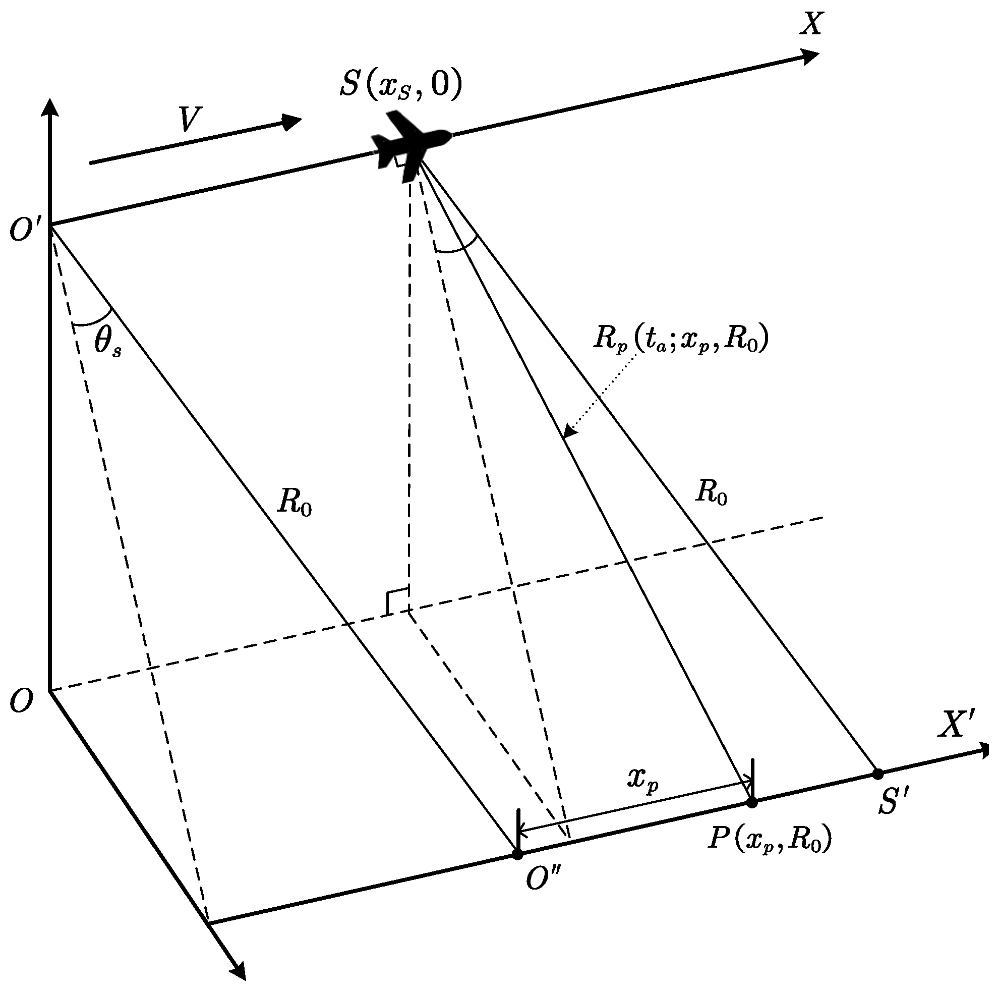
The squint imaging observation geometry is shown in Figure 1.

Figure 1.
Squint SAR imaging observation geometric model.
The coordinate system’s origin is positioned at the sub-satellite point, corresponding to where the SAR azimuth moment registers as zero, and X and are the azimuth axes of the SAR and the target, respectively. The SAR system travels along the X axis parallel to the axis at a speed of V. is the azimuth center position of the beam footprint, and is located at the starting point of the X axis. The real-time position of SAR is , where , is the azimuth slow time, and the straight line is parallel to the straight line . Assume that there is an observed object , where is defined as the range deviation between the center position of the beam and the target P, and is the shortest slant range between the observed object P and the X axis along the squint direction. Define the space squint angle as , then the instantaneous slant range at moment is:
where represents the azimuth position of point P, and expand Equation (1) to its Taylor series at the position :
where , and are called the linear range walk (LRW), the range cell curvature, and the cubic range migration term, respectively. Different from the side-looking and slight squint SAR, the slant range expansion term of a large squint SAR cannot be approximated by low-order approximation [8,11]. In high-resolution and large squint angle SAR, Equation (2) uses a third-order Taylor series approximation. Since the higher-order components are usually smaller than one range resolution unit, the higher-order components in the range migration can be ignored [27]. Moreover, the linear range walk term is much larger than the quadratic and above components, which will cause severe spectrum skew [28], resulting in a high azimuth sampling rate. SAR’s high squint angle characteristics are detrimental to deceptive jamming in terms of construction efficiency and construction difficulty. Assuming that the SAR system transmits a chirp signal, the echo signal of point P after demodulation can be expressed as:
where is the fast time, c is the speed of light, is the Doppler center time of the target P; is range window, is the antenna pattern in the azimuth direction. is the center frequency of the SAR, represents the wavelength, and is the modulation frequency of the chirp signal.
2.2. SAR Deceptive Jamming Model
According to the principle of SAR deceptive jamming [23,24], the modulation retransmission jammer intercepts the radar signal through modulation to restore the one-way propagation signal as Equation (3) and uses it as a jamming signal. The jamming signal is re-forwarded to the SAR system within a pulse repetition interval (PRI), thereby introducing false targets in the SAR image. The SAR deceptive jamming range-azimuth coordinate system is established, as shown in Figure 2.
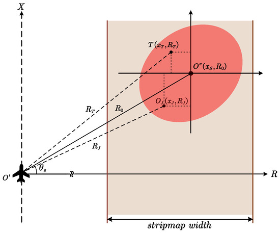
Figure 2.
Deceptive jamming model of squint angle SAR.
As shown in Figure 2, the X axis is the flight direction of the SAR system, the R axis is the direction of the slant range, and the origin of space is at the current position of the SAR system. The jammer is located at in the coordinate system, and represents the instantaneous slant range between the jammer and the SAR system. Use to represent any target point in the T area irradiated by the SAR beam, and its scattering coefficient is , represents the target point T and instantaneous slant range between SAR systems. Generally, the antenna beam of the SAR system is small, and the swath width is much smaller than the slant range length. Therefore, , , and the change of spatial squint angle can be neglected. If one wants to generate a target point in the T area by a jammer at the position, the modulation of the jammer can be modeled as a linear system as follows:
where is the range frequency, is the the synthetic aperture length, and
Then the frequency response function Equation (4) of the jammer can be decomposed into the position-dependent frequency response function of the jammer and the frequency response function of the SAR system with an integral term:
where is the frequency response function related to the jammer:
In addtion, is the frequency response function related to the SAR system:
Comparing Equations (7) and (8), it can be found that in the case of obtaining SAR-related parameters, the construction of can be completed only by pulse-by-pulse complex multiplication. The construction of occupies the main amount of computation in the construction of the JFR, and the slant range model under a large squint angle will also introduce complex range migration components. Therefore, how to construct efficiently and accurately is the key to completing the deceptive jamming of large squint SAR.
2.3. NLCSR-Based Deceptive Jamming
This section presents a systematic derivation of the NLCSR-based deceptive jamming algorithm for SAR systems with a large squint angle. Initially, the cross-coupling term’s consistent constructor is derived from separating the range walking term. Then, the constructor of the space-variant azimuth modulation term is derived in the azimuth time frequency transform domain through the non-linear chirp scaling method. Finally, the construction process of NLCSR-based SAR deceptive jamming is given.
2.3.1. Consistent Construction of the Cross-Coupling Term
The first exponential term is the LRW term. The LRW term has nothing to do with the double integral calculation, and the jammer can construct the LRW term together with in the range frequency domain through pulse-by-pulse complex multiplication. The construction function is as follows:
The second exponential term of Equation (11) can be equivalent to broadside R signal, and the platform flight speed is . The 2D spectrum of is shown in Figure 3b. The skew phenomenon is corrected, the degree of cross-coupling is significantly alleviated [28], and the effective azimuth sampling rate required for the signal is reduced.
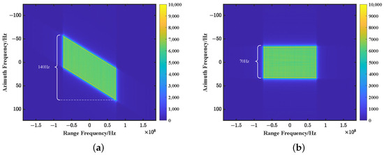
Figure 3.
Two-dimensional frequency domain signal simulation for single point target at a center frequency of 10 GHz, a squint angle of , a spatial resolution of 0.886 m, and a velocity of 100 m/s. (a) Raw 2D spectrum at large squint angle; (b) Two-dimensional spectrum at large squint angle after removing LRW term.
Convert Equation (11) to the 2D frequency domain by the principle of stationary phase [1]:
where represents the range frequency envelope. There are three exponential terms in Equation (12). The first index term is the displacement in the range direction. The second index term is the target azimuth position, which has nothing to do with the target azimuth position and squint angle. And the third term is the phase coupling term in the range direction and the azimuth direction. Expanding into a power series of yields
where
and
Among them, is the azimuth focusing modulation term. is the remaining range migration term after removing the LRW term. is the range modulation term caused by cross-coupling. is the high-order cross-coupling term. These complex cross-coupling terms have range dependence. Their precise construction necessitates the incorporation of complex interpolation and additional transform domain processing operations, which has low construction efficiency and high operational accuracy requirements [13,27,29]. Considering the high-efficiency requirement of deceptive jamming signal construction and the cross-coupling degree of has been reduced, and we propose a consistent construction method of the cross-coupling term based on reference slant range as follows:
where is the reference range of the jamming area. The reference slant range is used to uniformly construct the slant range dependent part of the cross-coupling term. The cross-coupling term can be constructed efficiently in the 2D frequency domain.
Removing the Equation (16) phase construction function, the construction of also leaves the remaining azimuthal modulation term. Perform range inverse Fourier transform on the remaining azimuth modulation term:
where is the bandwidth of the SAR signal, and the first exponential term represents a constant term, which has no effect on the focusing effect of the jamming signal. The second exponential term represents the azimuth position of the target. The third and fourth exponential terms represent the azimuth modulation term. Due to the misplacement of the slant range position of the missing linear range walk term, the azimuth spatial variability is increased. Therefore, the new slant range of the remaining azimuth modulation term is .
2.3.2. Construction of Azimuth Modulation Term Based on Non-Linear Chirp Scaling
Expanding the azimuth modulation term of the Equation (17) to its Taylor series at the position :
and
where is the azimuth modulation frequency. It can be seen from Equation (17) that the target point is located at the slant range of . However, the actual slant range position corresponding to the false target constructed by the deceptive jamming is , and the azimuth modulation terms of Equation (18) are also functions of the actual position . This is because Equation (10) separates the range walking term in the azimuth time-domain construction, which makes the jamming target point positioning abnormal. It can also be regarded as introducing the azimuth spatial variability of the azimuth modulation term. In order to express the spatial variability more clearly, put into Equation (18), we can get
and
where is the coefficient of the azimuth space-invariant term, and is the coefficient of the azimuth space-variant term.
In the construction of the azimuth modulation term, the higher the expected phase order is, the more complicated the construction process of the jamming signal is, which is not conducive to the efficient generation of the jamming signal. For the phase terms of cubic and above orders, we only consider constructing the azimuth space-variant part of the cubic phase. Therefore, the construction of the azimuth modulation term can be approximated as Equation (22).
where the constant exponential term has no effect on the jamming signal imaging and can be ignored. The quadratic coefficient is a function of the azimuth space-variant modulation frequency. In order to represent the spatial variability of the azimuth modulation frequency, the azimuth modulation frequency is expanded in terms of and keeps up to the second-order as
The modulation term coefficients of Equation (22) all have azimuth spatial variability, so their precise construction also needs to ensure the azimuth spatial variability of construction terms. In the existing deceptive jamming algorithm with a large squint angle, the construction of the azimuth modulation term is always calculated according to the range unit , and the spatial variable term related to cannot be generated [13,19]. These algorithms will lead to space-variant phase errors in the jamming signal, and the imaging quality of the jamming target will be degraded.
In this regard, we refer to the idea of compensating the space-variant term by the azimuth non-linear chirp scaling (ANCS) algorithm [27], and retain the spatial variability of the third-order term caused by removing the linear walk term. The non-linear chirp scaling compensation equations are established by the undetermined coefficients method. The compensation coefficients are solved, the jamming construction function is obtained by the inverse compensation function, and the azimuth modulation frequency and cubic modulation term with space variability are constructed.
In order to compensate for the cubic space-varying phase, the azimuth modulation term needs to be fourth-order filtered to provide enough parameters for solving the non-linear chirp scaling function. The azimuth fourth-order filter function can be expressed as:
where and are undetermined coefficients. Multiplying Equations (22) and (24), the azimuth space-variant modulatioin term can be expressed as
The Equation (25) is transformed into a 2D time domain expression by the principle of stationary phase:
It can be found that the non-linear chirp scaling signal form of Equation (26) is very similar to the range chirp scaling form in the chirp scaling imaging algorithm (CSA). Therefore, a non-linear chirp scaling function can be proposed to compensate for the spatial variability caused by the azimuth modulation frequency term and the azimuth cubic term.
For the denominator in the Equation (30), the second-order Taylor expansion can be performed at , respectively, and the Equation (30) can be written as a polynomial about and , and it can be obtained:
where is the space-invariant azimuth modulation term to be compressed. are the space-variant azimuth modulation terms. and have minimal effect on deceptive jamming imaging and can be ignored. The specific expressions of each coefficient are in Appendix A. To compensate for the spatial variability of these azimuth modulation terms, need to be compensated to zero. At the same time, need to be retained to ensure the focus of the target. Therefore, the following equations can be constructed to solve the undetermined coefficients of the fourth-order filtering function and the non-linear chirp scaling function:
where is a constant factor, solving this equation system can get the solutions of , , , , , and the solution process is shown in Appendix A. Then, the coefficients of functions and can be obtained. Bringing the above solution into Equation (29), the range-Doppler domain signal after compensation of the space-variant azimuth modulation term can be obtained:
It can be seen that the azimuth space-variant modulation term has been fully compensated by the fourth-order filter and the non-linear chirp scaling function. Conversely, the jamming construction function of the space-variant term can be obtained by the inverse process of compensation, as in Equation (34):
And the second exponential term in Equation (33) is the azimuth term to be compressed, which can be directly constructed in the azimuth frequency domain of the jamming signal, as in Equation (35):
Perform azimuth inverse Fourier transform on the remaining terms of Equation (33) to obtain a 2D time domain signal:
where is the Doppler bandwidth. This expression can be considered a collection of numerous scattering targets, and its essence is consistent with the SAR slant range image. Therefore, the SAR slant range image can be used to construct Equation (36), commonly referred to as the deceptive jamming template. However, in Equation (36), the position of the scattering targets, denoted as , deviates from the actual position of the scattering target within the deceptive jamming template. The set of scatters at this deviation position can be obtained by geometrically correcting the deceptive template:
- First, multiply the factor in the range frequency domain and azimuth time domain to achieve the range translation of the deceptive jamming template;
- Second, adjust the azimuth sampling interval of the deceptive template, divide the original sampling interval by to achieve the azimuth scaling of the deceptive jamming template, and the Equation (36) can be obtained.
To sum up, represents the deceptive jamming template after geometric correction. After inputting the deceptive jamming template of geometric correction, the construction of the JFR for large squint SAR can be realized by the following expression:
where is the azimuth Fourier transform, is the inverse Fourier transform of the azimuth, and is the range Fourier transform. As evident from Equation (37), constructing the SAR JFR for a large squint angle requires Fourier transform and complex multiplication computations. The algorithm flow is simple and efficient.
2.3.3. Construction Process of Jamming Signal Based on NLCSR Algorithm
In this subsection, the workflow of the NLCSR deceptive jamming algorithm is described. First, the jamming frequency response generation process in the NLCSR algorithm is introduced according to Equation (36). Then, the workflow of applying the NLCSR algorithm to actual SAR jamming systems is given.
In the signal construction process of SAR deceptive jamming with a large squint angle, it is necessary to obtain the relevant parameters of jamming in advance, mainly including the following aspects:
- SAR signal parameters, such as center frequency , signal bandwidth , signal pulse width , and pulse repetition frequency ;
- SAR antenna parameters, such as synthetic aperture length , squint angle and pitch angle ;
- SAR platform parameters, such as flight speed V, and SAR flight height H.
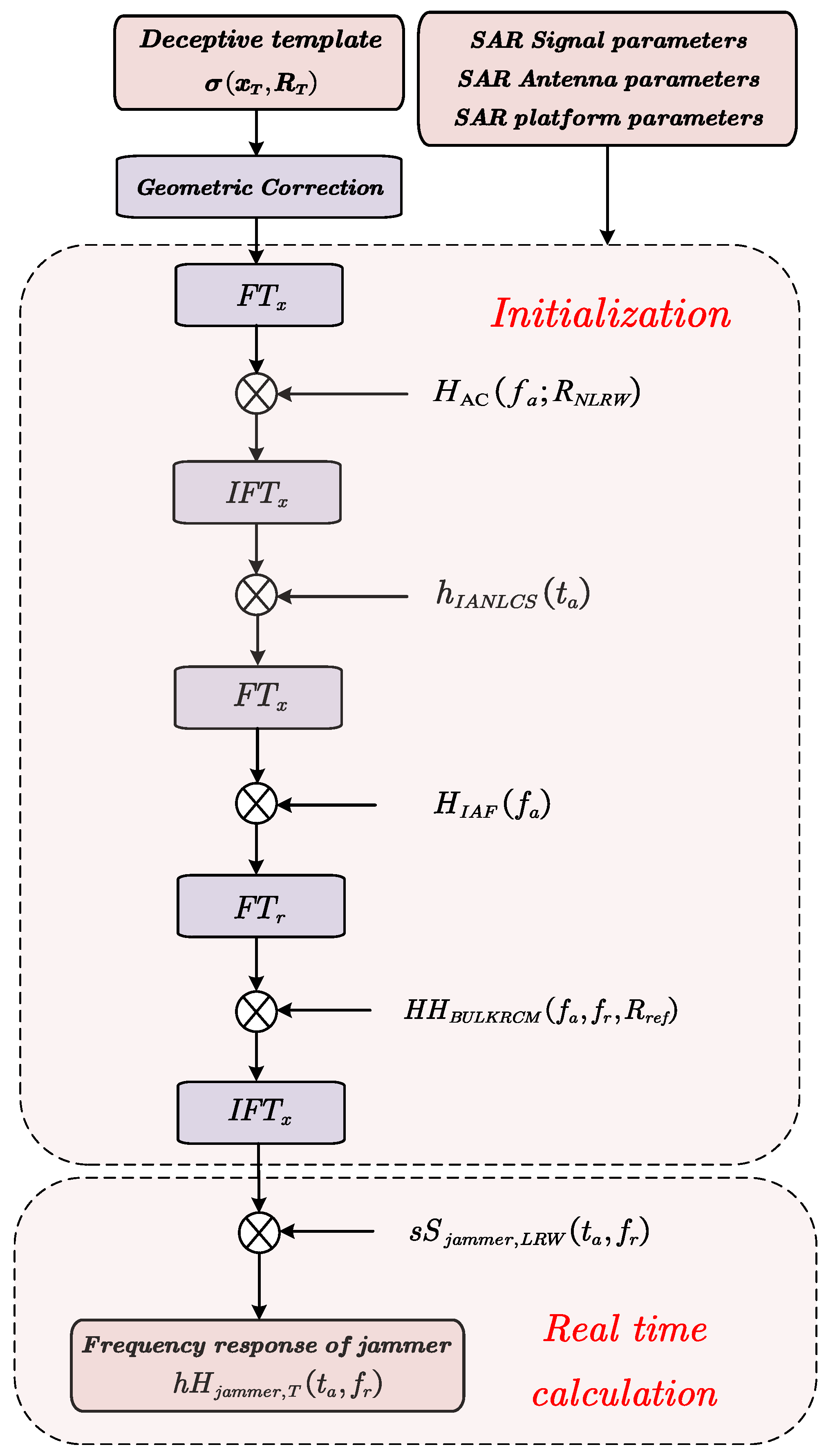
The topic of this article is not to discuss how to obtain these parameters. It is assumed that these parameters have been obtained through reconnaissance signal processing. The workflow of the NLCSR-based SAR deceptive jamming algorithm with a large squint angle is shown in Figure 4, which mainly includes two stages: jamming initialization and real-time modulation calculation.
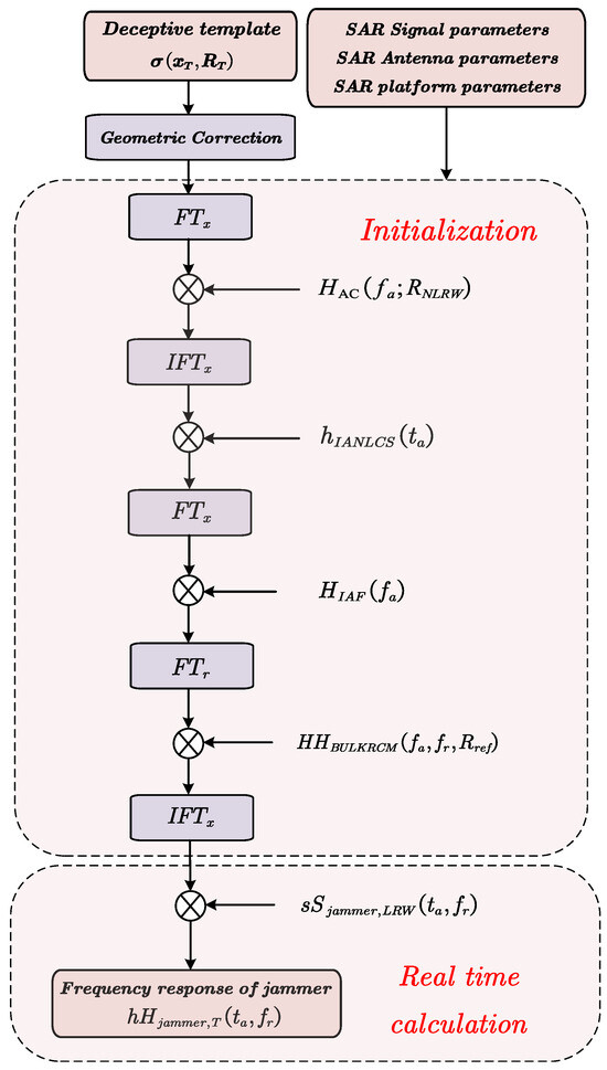
Figure 4.
The workflow of large squint SAR deceptive jamming algorithm based on non-linear chirp scaling and low azimuth sampling reconstruction (NLCSR).
The first stage is the initialization of the jammer. Firstly, the deceptive template with complex backscattering coefficients is prepared. The set of scatters for the desired offsets is then obtained by geometrically correcting the deceptive template. According to the acquired SAR parameters, the jammer first performs non-linear chirp scaling in the 2D time domain and the range-Doppler domain to construct the azimuth modulation term for generating the jamming signal. Then, the azimuth modulation term converts into the 2D frequency domain, constructing the jamming signal cross-coupling term.
The second stage is the real-time computing stage. The LRW term of the jamming signal is constructed in the range frequency domain so that the SAR system frequency response function of the current pulse time can be constructed. Finally, combine the jammer position-related frequency response function to get the JFR at the current pulse time.
In the above steps, it can be observed that the NLCSR algorithm only accomplishes the calculation through Fourier transform and complex multiplication during the construction of the jamming signal. The NLCSR algorithm possesses the characteristics of simple implementation and high imaging efficiency. Moreover, as shown in Figure 3, since the main computation of the algorithm is calculated without considering the LRW term, the JFR construction in the initialization stage can adopt a lower azimuth oversampling rate, which can significantly reduce the calculation amount in the initialization stage. The azimuth sampling rate after downsampling can be expressed as follows:
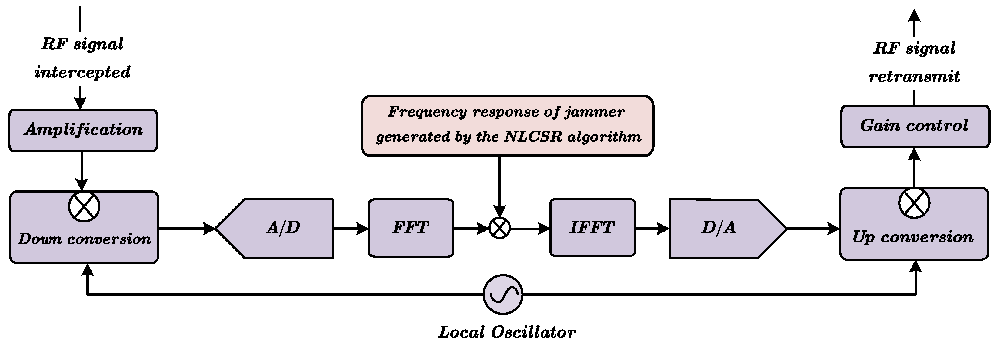
Before the real-time modulation calculation, zero-filling in the frequency domain can avoid the azimuth aliasing effect, which reduces the calculation burden. In actual SAR jamming, the real-time modulation stage of the NLCSR algorithm needs to be combined with the digital radio frequency memory (DRFM), as shown in Figure 5. The jammer needs to undertake amplification, down-conversion, analog to digital (A/D) conversion, and Fourier transform of the intercepted SAR radar signal to obtain the baseband range frequency domain signal, multiply it with the jamming frequency response (JFR), and then perform inverse Fourier transform, digital to analog (D/A) conversion, up-conversion, and gain control to generate the jamming signal and forward it to the SAR radar. Therefore, the NLCSR algorithm, which mainly uses Fourier transform and complex multiplication as its main calculation methods, is more suitable for a DRFM-based jamming system, thereby achieving efficient SAR deceptive jamming with low azimuth sampling.

Figure 5.
The structure of SAR deceptive jamming based on modulation retransmission.
3. Analysis and Simulation of NLCSR Algorithm
This section proves the effectiveness of the NLCSR algorithm through the jamming signal imaging simulation and analysis.
3.1. Simulation and Result
This section conducts a jamming simulation for the SAR system in Table 1. The validity of the NLCSR algorithm is demonstrated through jamming simulations of false targets and real scene data.

Table 1.
Parameters of simulation.
3.1.1. False Point Target Simulation
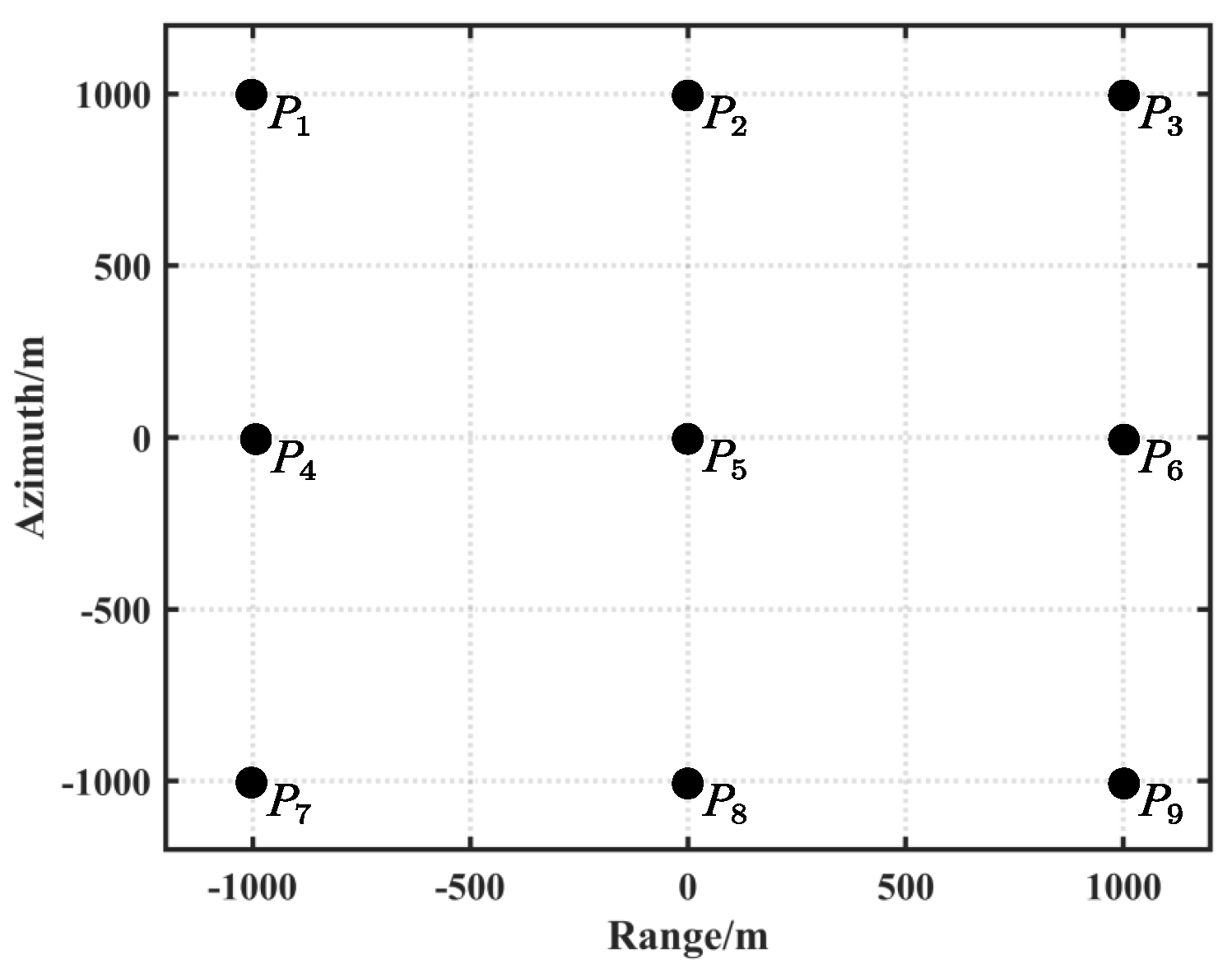
In order to analyze the jamming signal construction quality of the NLCSR algorithm accurately, the jamming template for the false targets is established by setting a point target array with a uniform spacing of 1 km. The simulation scene covers an area of 2 km km, as shown in Figure 6, in which nine point targets are set in the strip. The jammer is set at point .
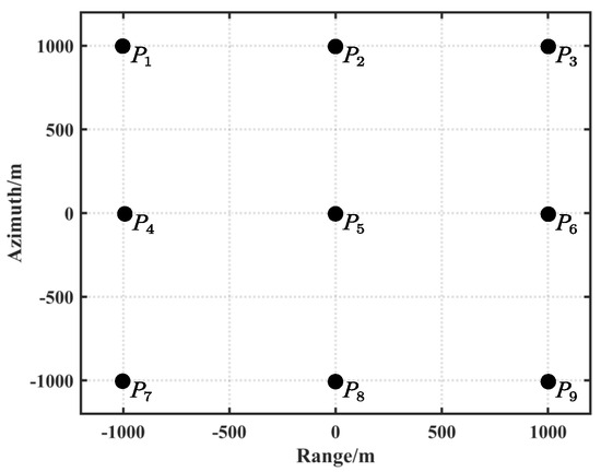
Figure 6.
Deceptive jamming false target template.
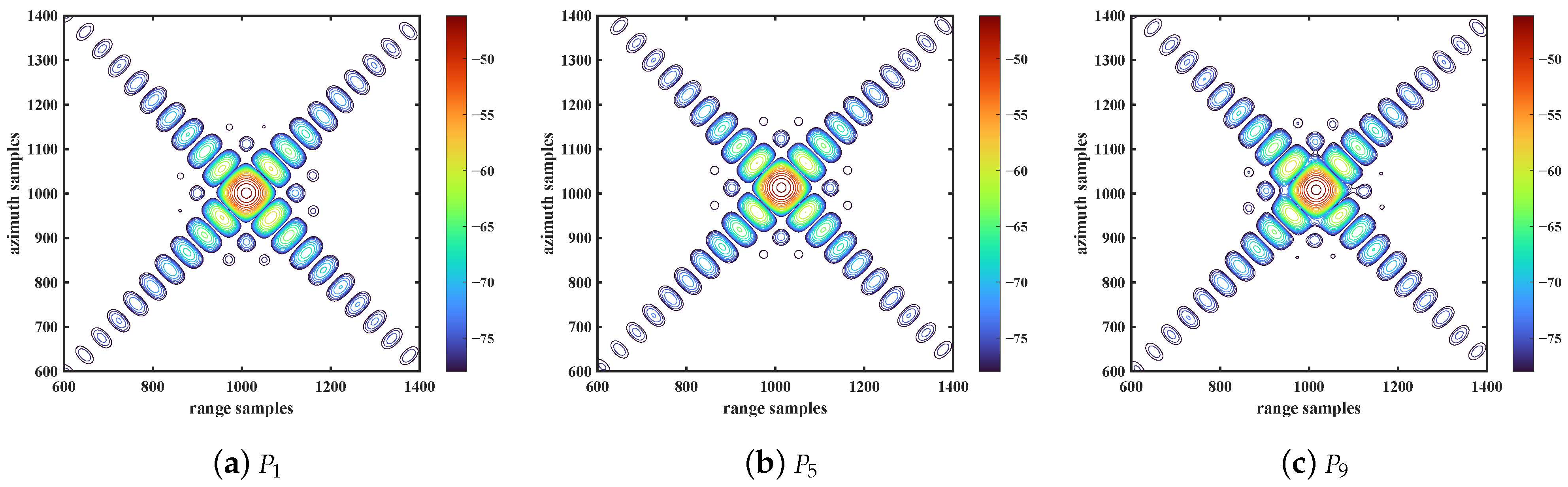
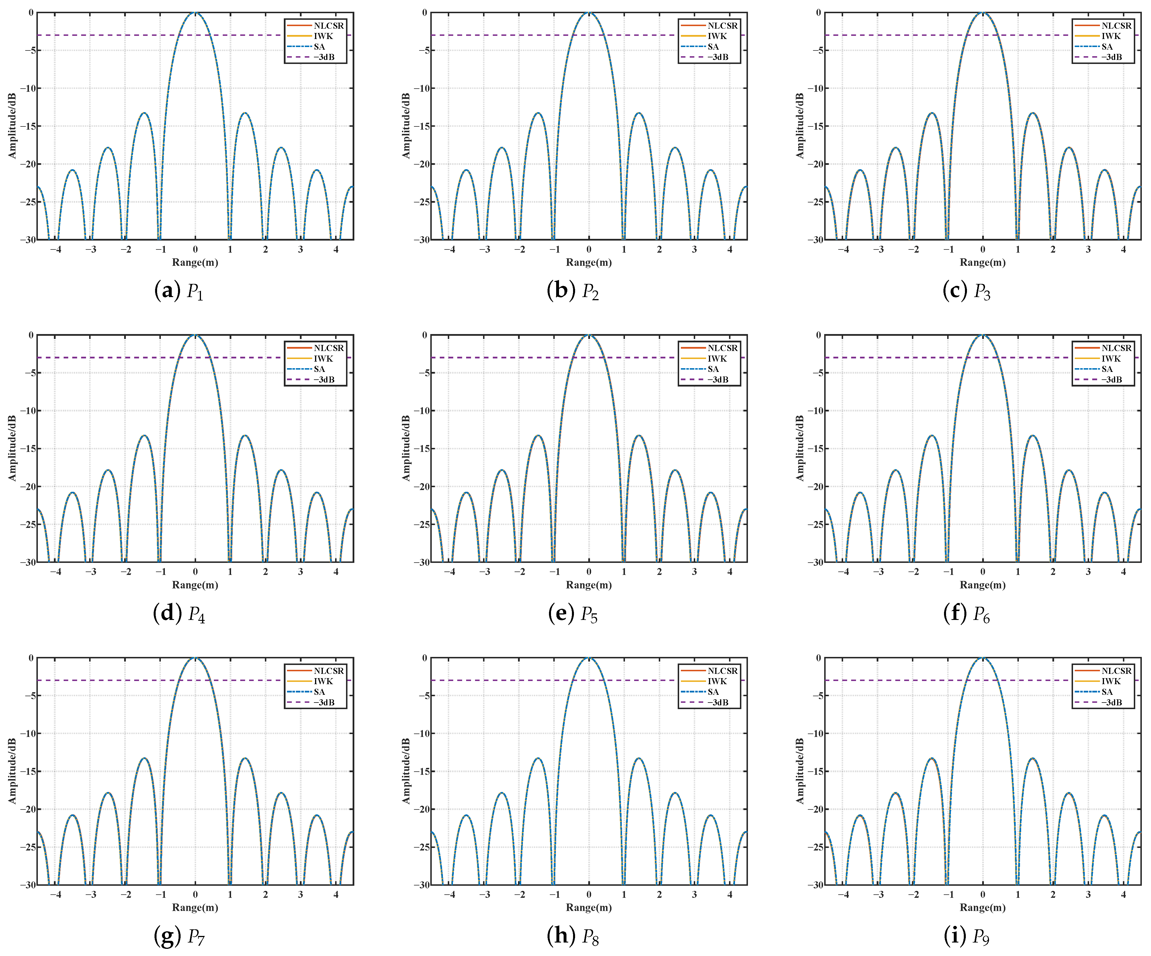
To analyze the focusing characteristics of the jamming signal in detail, Figure 7 shows the imaging close-up images in the strip mode with a large squint angle. The focusing effect of false targets at different range and azimuth positions is good, and the deflection angle of the focusing sidelobe is correct. The point-by-point superposition calculation algorithm (SA) and IK algorithm that adapt to large squint SAR jamming are also used for comparison and simulation. All false point targets’ range and azimuth profiles are analyzed, as depicted in Figure 8 and Figure 9.
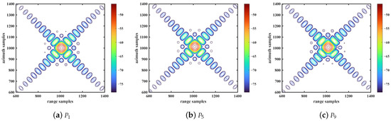
Figure 7.
Close-up images of the fake target template. Subfigures in each of three columns (from left to right) are the images of , and , respectively.
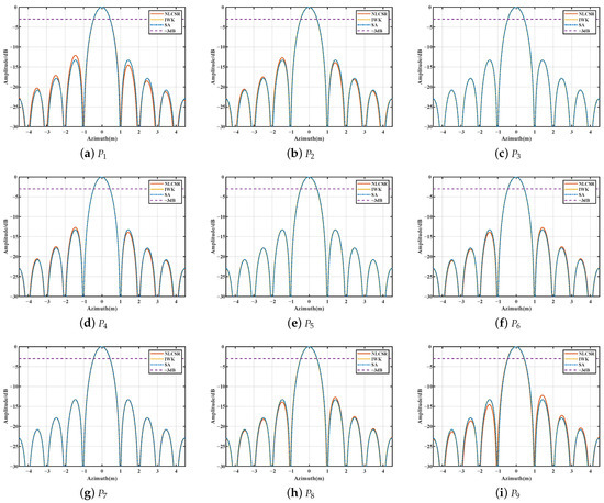
Figure 8.
Range profiles of the false point targets generated using SA, IK, and NLCSR. (a–i) Range profiles of scatterers –.
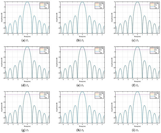
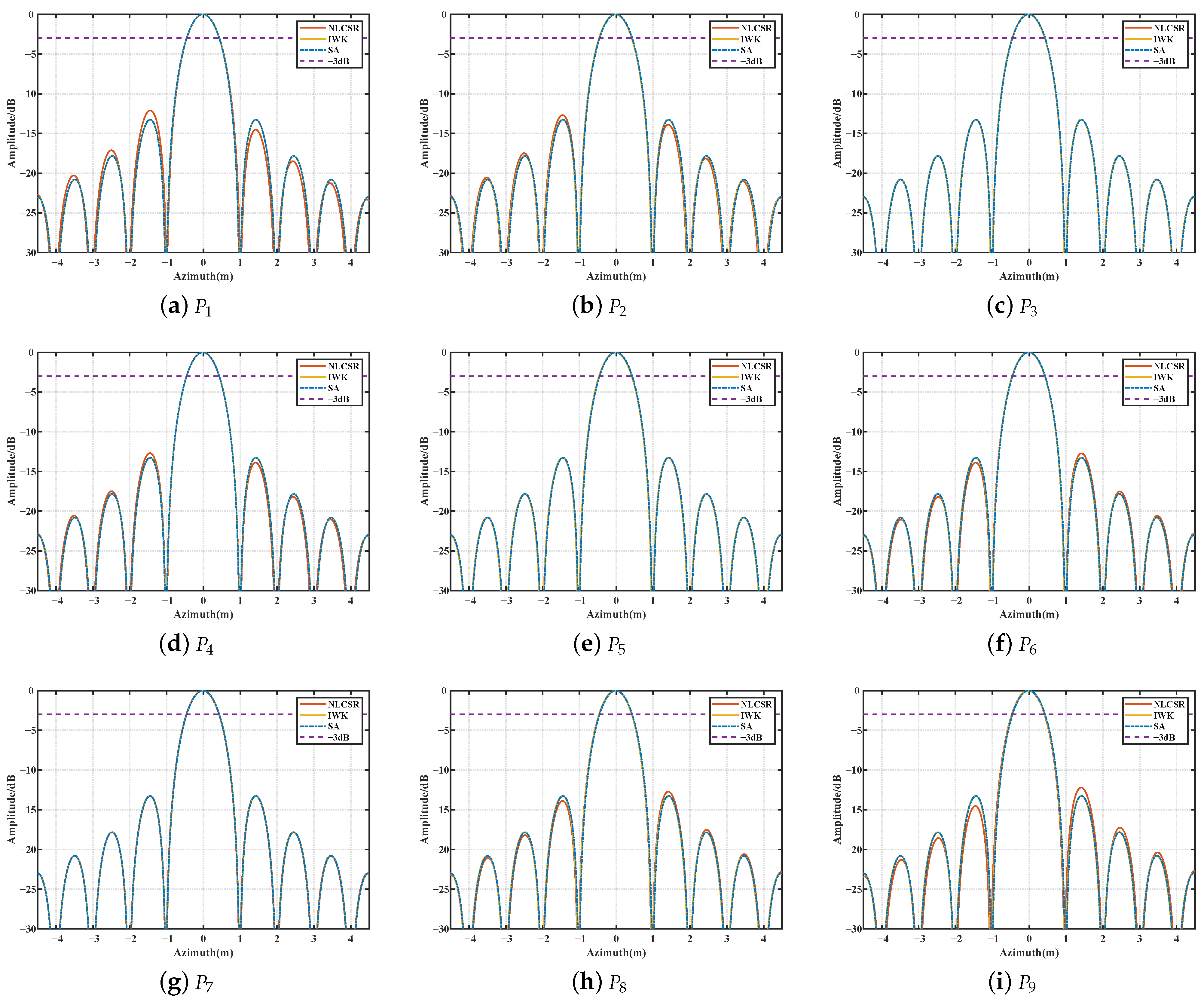
Figure 9.
Azimuth profiles of the false point targets generated using SA, IK, and NLCSR. (a–i) Azimuth profiles of scatterers –.
The range-azimuth imaging contour of the SA algorithm is represented by the dotted blue line, serving as a benchmark for standard point targets. The solid orange line is the range-azimuth imaging contour of the IK algorithm, and the solid red line is the range-azimuth imaging contour of the NLCSR algorithm. The three methods’ 3 dB impulse response width (IRW) is almost identical. The first sidelobe of the false jamming target by the NLCSR algorithm appears asymmetrical, which affects the calculation of the peak sidelobe ratio, but this has little effect on the resolution.
Table 2 presents the imaging quality indexes for all point targets, encompassing the 3 dB impulse response width (IRW), peak sidelobe ratio (PSLR), and integral sidelobe ratio (ISLR). As depicted in the table, the range and azimuth IRW for the SA algorithm false targets amount to 0.8860 m and 0.8860 m, respectively. In the range direction, the maximum broadening of false targets generated by the NLCSR algorithm is . Similarly, in the azimuth direction, the maximum broadening of the false target is , and the influence of broadening is almost negligible. The jamming accuracy of the false target generated by the NLCSR algorithm is almost the same as that of the IK algorithm. The algorithm does not use the interpolation processing method, so jamming modulation processing is more accessible, and transform domain Fourier transform and complex multiplication operations are more convenient for algorithm expansion and function integration.
Table 2.
Comparison of Imaging Quality Indexes among Different Algorithms.
3.1.2. Actual Scene Deceptive Simulation
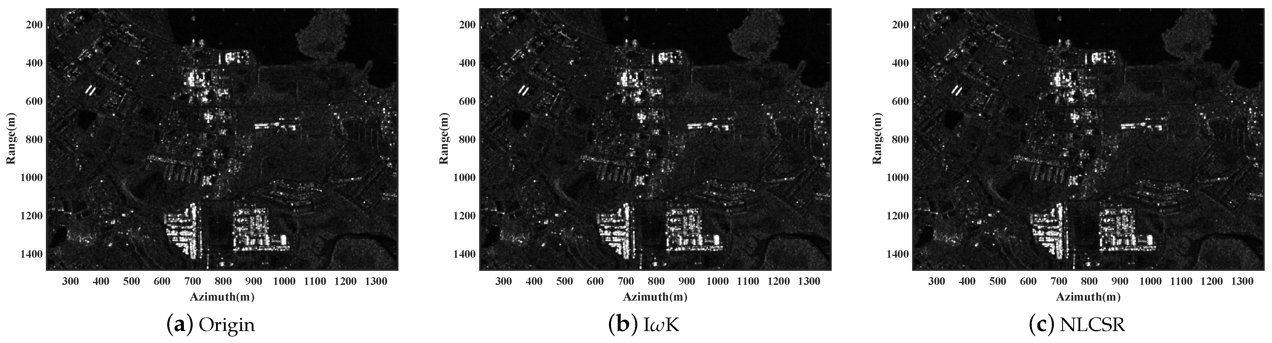
In this section, the actual ground scene is used as a deceptive template, and the deceptive jamming of SAR with a large squint angle is carried out through the NLCSR algorithm. SAR images were selected as deceptive templates in the public dataset of the TerraSAR-X system [30], and the NLCSR algorithm and IWK algorithm were used to generate jamming signals to obtain false scenes after imaging. The false scene imaging results were compared with the original SAR images to prove the focusing ability of the NLCSR algorithm. The simulation test parameters are shown in Table 1. The original scene deceptive template and the jamming imaging fake scenes are shown in Figure 10. From the perspective of the SAR image, the NLCSR algorithm demonstrates a high level of similarity with the original SAR image.
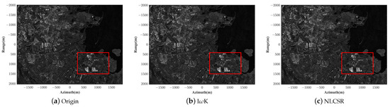
Figure 10.
Actual images of the real scene. (a) The origin deceptive template; (b) fake scene generated using IK; (c) fake scene generated using NLCSR.
In order to elucidate the specific dissimilarities, an enlargement of the region inside the red box, measuring km × km, is presented in Figure 11. Furthermore, the structural similarity (SSIM) metric was employed to assess the disparities between the fake scene and the actual scene, thereby evaluating the deceptive jamming quality. The SSIM was for the fake scene based on the IK algorithm and for the fake scene based on the NLCSR algorithm, which is nearly identical. Comparing the point target imaging indicators and the deceptive scene structural similarity shows that the approximation processing in the NLCSR algorithm will bring about partial focus loss, which will increase as the distance away from the deceptive jamming center increases. However, the imaging results indicate a remarkable similarity between the jamming signal of the NLCSR algorithm and the original SAR signal, the approximation error caused by the NLCSR algorithm is almost indistinguishable from the IK algorithm and the original signal, and the electromagnetic characteristics of the deceptive template can be well preserved.
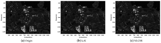
Figure 11.
Region enlargement comparison in red boxes of Figure 10. (a) The origin deceptive template; (b) fake scene generated using IK; (c) fake scene generated using NLCSR.
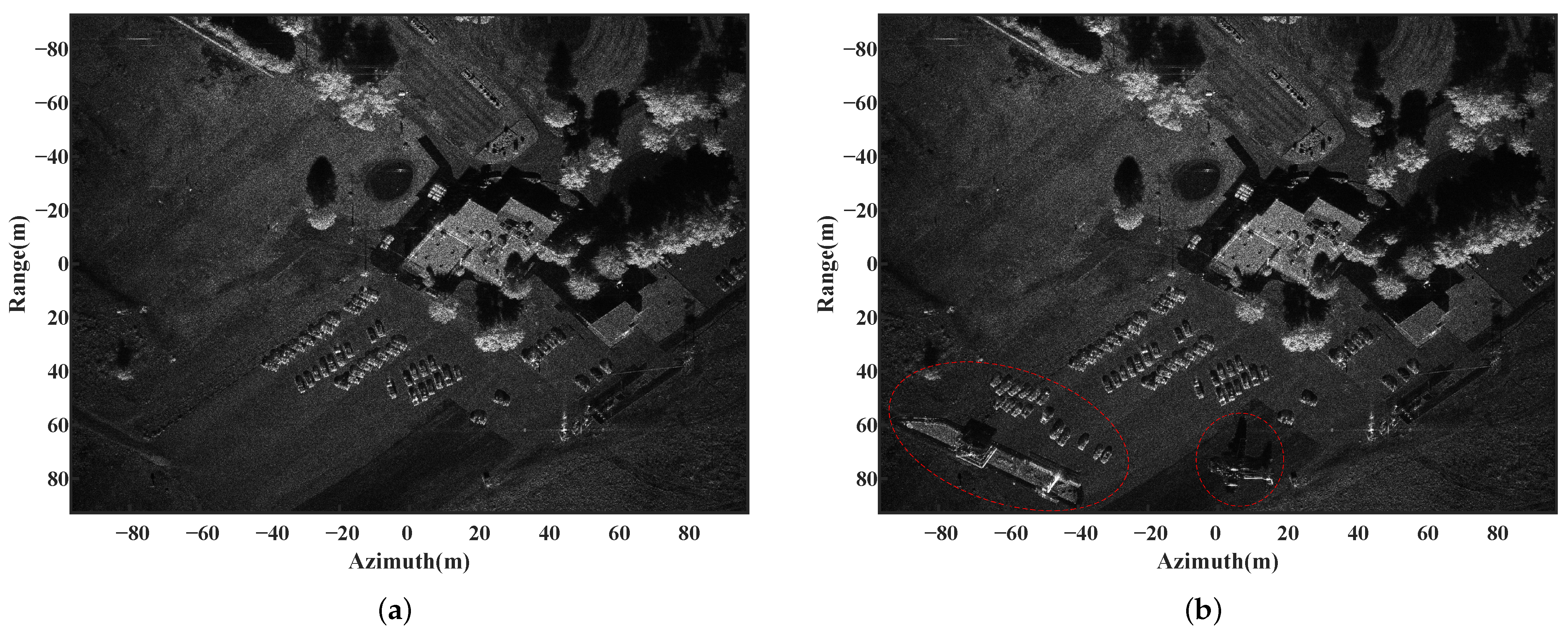
Finally, the camouflage deceptive jamming simulation of the real echo scenario is performed. SAR image is selected from the public SAR data of Sandia National Laboratory in the United States as natural scenes to generate echo signals [31]. Then, select × parking lot and × aircraft image as the deceptive template in another SAR image, and use the NLCSR algorithm to generate the deceptive jamming signal so as to realize false target and fake scene camouflage effects in real scene echo imaging. The real echo scenario imaging is shown in the Figure 12a. Figure 12b shows the results of jamming imaging.
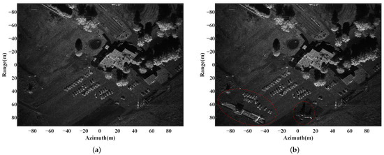
Figure 12.
Deceptive jamming simulation in actual scene. (a) Imaging result of the actual scene echo; (b) imaging result after adding the jamming signal to the echo by NLCSR.
Compared to the actual scene in Figure 12a, the false parking lots and airplane demonstrate a high degree of focus, rendering it arduous to discern from the actual scene. The jamming simulation results prove the effectiveness of the NLCSR algorithm.
3.2. Validity Analysis
First, the validity of the approximate conditions of the NLCSR algorithm is analyzed. The model construction of the jamming signal model will be analyzed, respectively, and the constraints of the algorithm will be listed.
3.2.1. Validation of the Cross-Coupling Signal Model
In the consistent construction of the cross-coupling term, the remaining range migration term, range modulation term, and high-order cross-coupling term are constructed by the reference slant range . However, in Equation (20), these remaining terms are all range space-variant. When the maximum difference in range upward exceeds a certain error tolerance, the space variation cannot be ignored and must perform space-variant compensation for the cross-coupling term.
Here, we analyze the range-dependent characteristics of the residual range migration term, range modulation term, and high-order cross-coupling term on azimuth frequency. Considering a m resolution X-band SAR system with a squint angle of , the reference slant range is 22.75 km, and the false targets with the actual slant range of km, km, and km are generated by NLCSR algorithm. The error caused by the consistent construction of the cross-coupling term is analyzed. Since the high-order cross-coupling term is very small [28,29], only the range-dependent characteristics of the remaining range migration term and the range modulation term are considered here.
Figure 13b demonstrates that the phase error induced by the construction of the range modulation term for the target remains considerably smaller than , so the range dependence of the range modulation term can be ignored. However, as shown in Figure 13a, when the difference between the actual slant range of the false targets and the reference slant range is greater than 4 km, its residual range migration will exceed range resolution units. Therefore, when jamming against SAR with a wide swath greater than 8 km, due to the range dependence of the remaining range migration term, it is impossible to construct accurate coupling terms for all targets at different ranges in the 2D frequency domain. In this article, the construction strategy of scene range block processing is adopted. According to the imaging focusing condition, the residual range migration error is limited to a specific range in a range processing sub-block. Finally, the width of the range processing sub-block can be determined by the error limit range. The residual range migration error is expressed as:
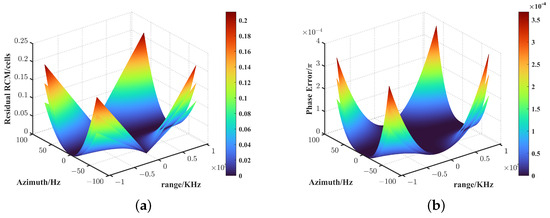
Figure 13.
Error simulation of residual range migration term and range modulation term at a center frequency of 10 GHz, a squint angle of , a spatial resolution of m, and a velocity of 100 m/s. (a) Residual range migration term; (b) range modulation term.
During the imaging processing of the jamming signal, it is essential to ensure the residual range migration term remains below range resolution unit so that the following equation can be obtained:
Assuming that the solution of the above inequality Equation (40) is , the length of the range direction processing block is as:
The above expression is calculated when the SAR meets the center frequency of 10 GHz, a squint angle of , and a spatial resolution of m. When the width of the range processing sub-block is controlled m, the remaining range migration error is less than resolution units, and the phase error caused by the construction of the range modulation term is much smaller than . Therefore, the range space-variant cross-coupling term can be constructed by the consistent construction of the cross-coupling term.
3.2.2. Validation of the Azimuth Signal Model
In the construction of the azimuth modulation term, in order to simplify the construction and calculation of the azimuth modulation term, the high-order space-variant phase of the azimuth modulation term is approximated, such as Equation (22). This approximation error can be equivalent to the residual uncompensated azimuth space-variant modulation term after the imaging processing of the jamming signal, which will affect the focusing depth of the deceptive jamming target. The approximation error can be expressed as:
According to the above Equation (42), we simulate and analyze the residual azimuth spatial variability of the approximation error. Figure 13 shows false targets’ residual space-variant phase error variation at different azimuth positions, azimuth resolutions, and squint angles.
It can be seen from the figure that as the false target azimuth position increases relative to the deceptive jamming azimuth center position, and the phase error becomes larger, which is consistent with the analysis results of dot matrix false target imaging indexes in Table 2. Moreover, the large squint angle and the high resolution will aggravate the phase error of the azimuth modulation term constructed.
In Equation (23), the space-variant azimuth modulation frequency is approximated. This approximation will produce a quadratic phase error (QPE), affecting the azimuth focusing depth. The quadratic phase error can be expressed as:
According to the above Equation (43), we simulated the quadratic phase error, as shown in Figure 14. The approximate phase error change of the azimuth space-variant modulation frequency with the azimuth resolution and squint angle is given when the deceptive jamming target is in different azimuth positions.
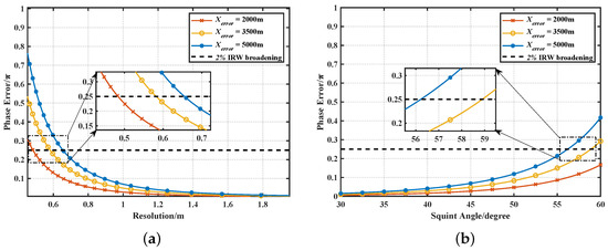
Figure 14.
Error simulation of the high-order pre-filter in azimuth frequency domain. (a) SAR system at a center frequency of 10 GHz, a squint angle of , and a velocity of 100 m/s; (b) SAR system at a center frequency of 10 GHz, a spatial resolution of m, and a velocity of 100 m/s.
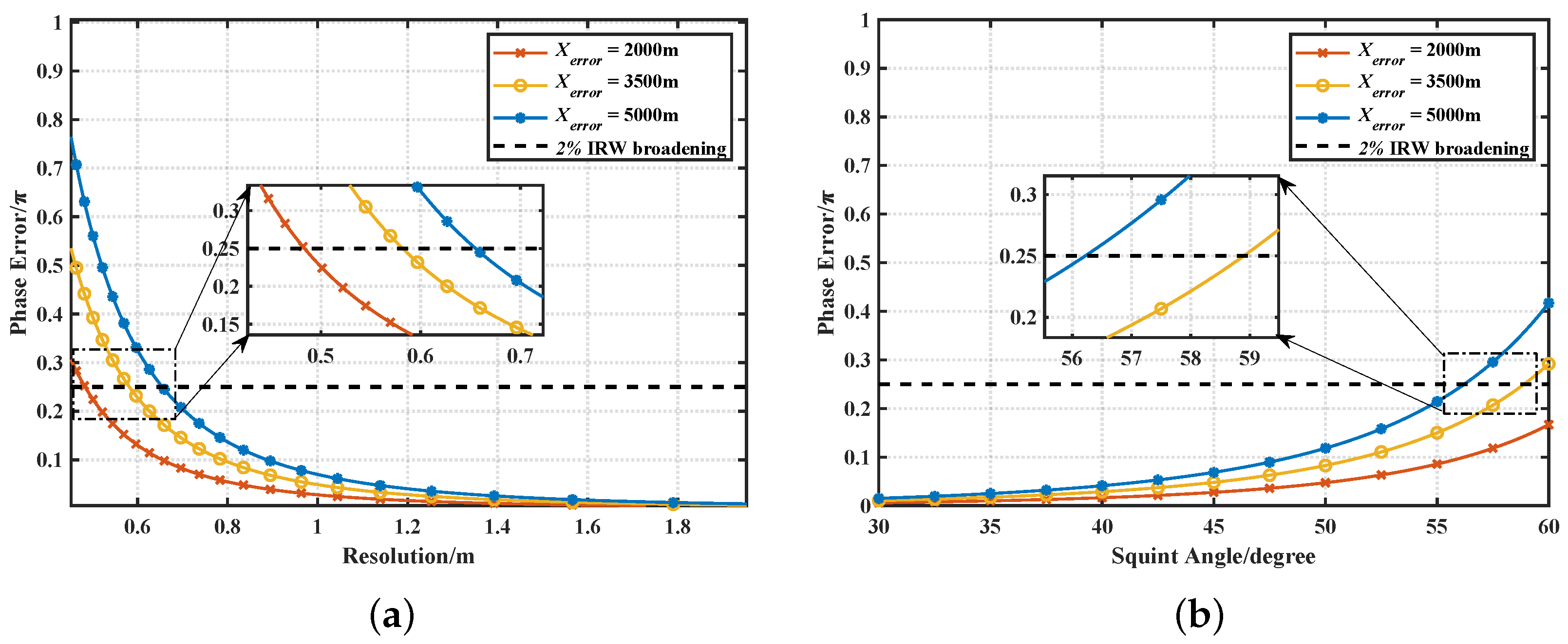
It can be seen from Figure 15 that as the false target azimuth position increases relative to the deceptive jamming azimuth center position, the greater the phase error constructed by the azimuth modulation frequency term. It can be concluded that the NLCSR algorithm can be adapted to high-resolution SAR systems with a resolution of m and a squint angle of when the range of deceptive jamming azimuth is less than 4 km. When the jamming target is a SAR system with an azimuth resolution of 1 m and a large squint angle of , the range of deceptive jamming can be increased to 7 km. Therefore, the NLCSR algorithm can realize high-precision SAR deceptive jamming with a large squint angle.
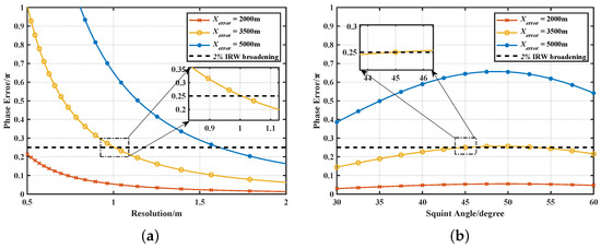
Figure 15.
Approximation error simulation of the azimuth modulation frequency term. (a) SAR system at a center frequency of 10 GHz, a squint angle of , and a velocity of 100 m/s; (b) SAR system at a center frequency of 10 GHz, a spatial resolution of m, and a velocity of 100 m/s.
Suppose there is a higher requirement for the imaging accuracy of the algorithm. In that case, the width of the range processing sub-block can be controlled smaller, and a higher-order azimuth modulation term can be considered. However, it should be noted that the more the range processing sub-blocks are considered, the higher the approximation processing order and the more complex the subsequent jamming signal construction process will be. Under actual conditions, a reasonable choice should be made for the accuracy and efficiency of jamming signal construction according to the performance of the specific jamming SAR system.
3.3. Computational Complexity Analysis
This section will analyze the computational complexity of the NLCSR algorithm. For the convenience of analysis, operations such as addition, multiplication, and square root used by the algorithm are considered basic operations that can be performed in one instruction cycle. The deceptive template is assumed to comprise scatter points, where M represents the number of azimuth units and N represents the number of range units. Furthermore, the NLCSR algorithm’s jamming modulation encompasses the amount of SAR signal range sampling points, denoted as , and azimuth sampling points denoted as .
Analyze the basic operation in the main workflow of Figure 4. First, the calculation of the geometric correction of the deceptive template requires basic operations, which can be performed in offline preparation. In the initialization stage, the construction part of the azimuth modulation term mainly needs the azimuth Fourier transform and complex multiplication operation. The corrected deceptive template constructs the second-order azimuth frequency modulation term, which requires basic operations. It takes basic operations to construct the azimuth space-variant high-order modulation term. The construction part of the range modulation term mainly needs the range Fourier transform, the azimuth Fourier transform, and the complex multiplication operation. The consistent construction of the cross-coupling term requires basic operations. According to the Equation (38), the initialization phase of the NLCSR algorithm can be calculated at a low azimuth sampling rate, and the number of new sampling points in the azimuth direction is . Therefore, the amount of computation in the initialization stage is:
In the real-time calculation stage, the jammer needs to extract the data of the initialization template pulse by pulse for processing. The construction of the linear distance walking item and the operation of the jammer position-related frequency response function on the distance dimension data require basic operations. Furthermore, the frequency-domain circular convolution of DRFM requires basic operations. Therefore, the amount of computation in the real-time computing stage is:
The traits of the NLCSR algorithm can be synthesized based on the analysis mentioned above. In the entire jamming signal construction calculation, the primary computational workload of the NLCSR algorithm is the Fourier transform. In the same way, the IK and SA algorithms that can adapt to SAR deceptive jamming imaging at large oblique angles of view are analyzed, as shown in Table 3.
Table 3.
Computation amount comparison of different algorithms.
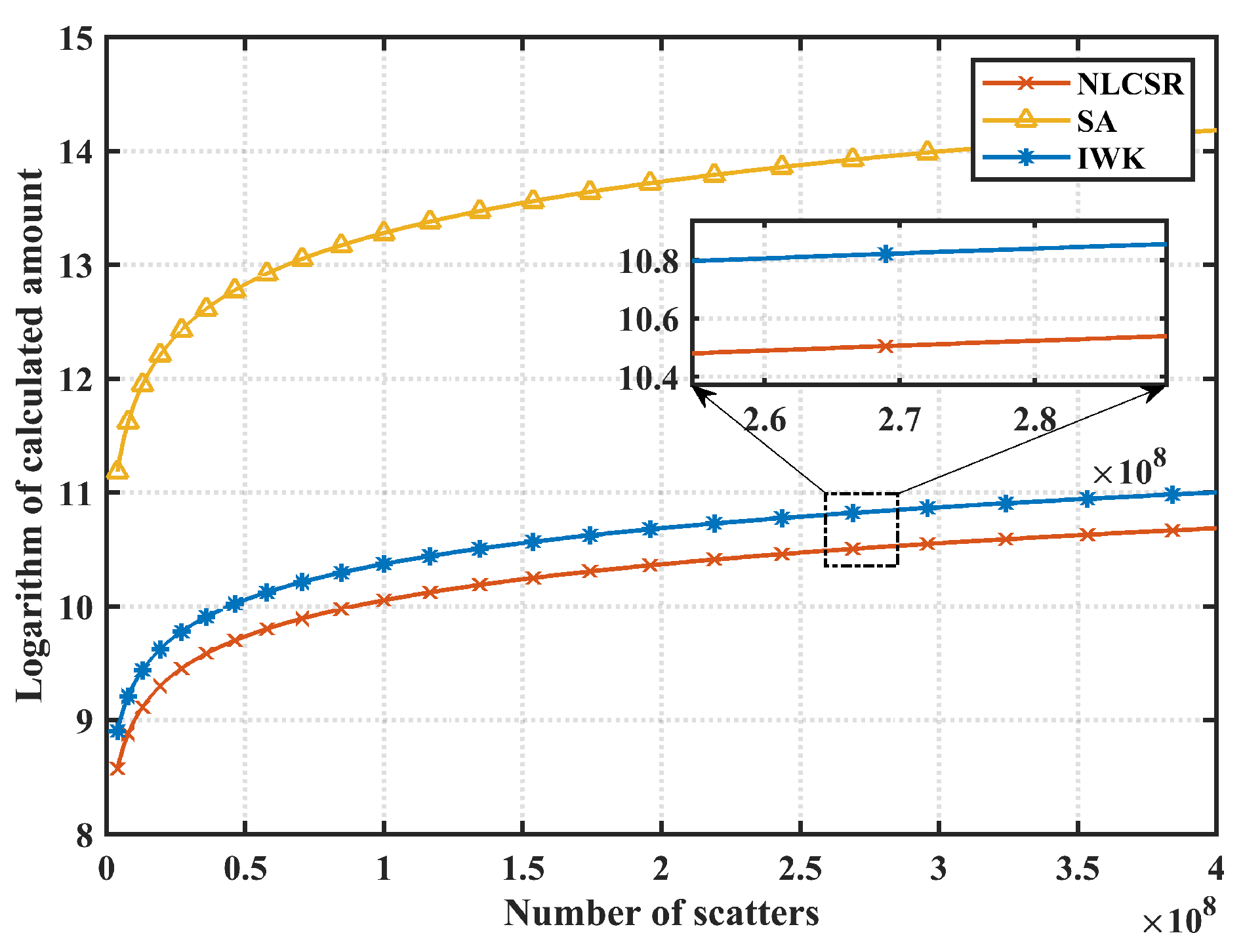
To facilitate a visual comparison of the computational complexity between these algorithms, we keep the parameters controlled as and plot a logarithmic graph depicting the total count of basic operations for each algorithm, as shown in Figure 16.
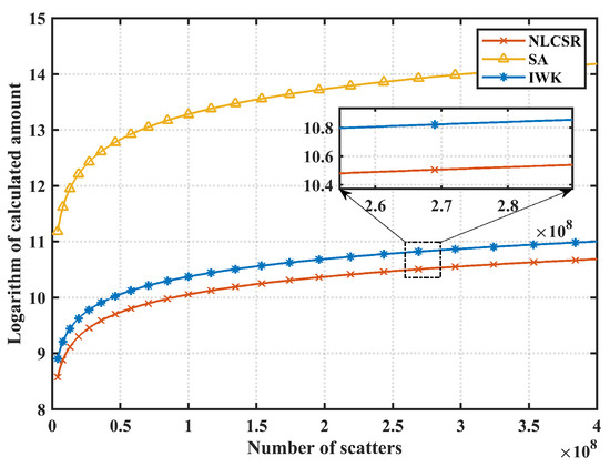
Figure 16.
The relationship between the basic operation amount and the total number of scatters in the template.
It is evident that the NLCSR algorithm demonstrates the lowest count of basic operations. After calculation and comparison, the jamming modulation efficiency of the NLCSR algorithm is higher than that of the IK algorithm. Moreover, the modulation operation of the NLCSR algorithm only needs Fourier transform and complex multiplication operation, which is simple and efficient, avoids the phase loss and Gibbs phenomenon caused by the interpolation operation [1,26], and is easy to use in the FFT-based signal processors and parallel processors realized.
The average running time simulation experiment was conducted on a computer equipped with a CPU with a main frequency of GHz. We used Matlab2021a to simulate three kinds of SAR deceptive jamming algorithms with large squint angles. We also calculated the average running time under different deceptive template sizes and signal sampling points, as shown in Table 4. The NLCSR algorithm takes the least time for jamming modulation. In addition, due to the low efficiency of the MATLAB interpreter using different degrees of optimization algorithms, the running time simulation did not exactly match the computational complexity analysis. By utilizing a field programmable gate array or a parallel digital signal processor implemented with FFT, the processing speed can be enhanced over tenfold, while simultaneously ensuring fulfillment of real-time constraints. Based on the above analysis, the NLCSR algorithm has more advantages in computational complexity.
Table 4.
Average Running Time of Different Algorithms.
4. Discussion
From the analysis and experimental results in Section 3, it can be seen that the NLCSR SAR deceptive jamming algorithm with a large squint angle can meet the jamming focusing ability and computational efficiency at the same time. Moreover, the algorithm suits SAR deceptive jamming with side-looking and small squint angles. However, the proposed method still has some problems.
As in the effectiveness analysis in Section 3.2, the NLCSR algorithm makes an approximation of balancing computational efficiency in the construction of the high-order cross-coupling phase term and the construction of the azimuth high-order modulation term. These approximations will limit the NLCSR algorithm’s adaptation to SAR system parameters, and the squint angle, resolution, and azimuth jamming range of deceptive jamming adaptation are mutually restricted. Suppose it is desired to satisfy higher-resolution SAR deceptive jamming with a large squint angle. In that case, limiting the azimuth jamming range and squint angle of deceptive jamming is necessary. Regarding the limitation of the effectiveness of the jamming as mentioned in relation to the above targets and the requirement of SAR multi-imaging mode jamming, how to improve the adaptability of the algorithm without increasing the complexity of jamming signal construction is a problem that we need to study further.
5. Conclusions
This article mainly studies the problem of SAR deceptive jamming with a large squint angle. Aiming at the dilemma of not being able to consider both jamming calculation efficiency and accuracy, an efficient large squint SAR deceptive jamming algorithm based on non-linear chirp scaling and low azimuth sampling reconstruction is proposed. The algorithm adopts the idea of constructing the JFR in the transform domain. It completes the construction of a high-precision signal model under the condition of removing the linear range walking term and low azimuth sampling. Therefore, the workflow of the NLCSR algorithm only needs Fourier transform and complex multiplication, which is easier to implement in hardware than interpolation. Simulation results prove that the NLCSR algorithm has a notable advantage in the efficiency of jamming signal construction compared to the existing deceptive jamming algorithm while ensuring the high-precision jamming signal focusing ability. In addition, we also explore the adaptability of the NLCSR algorithm and summarize the validation of the algorithm. The advantages of high accuracy and high efficiency give the NLCSR large squint angle SAR deceptive jamming algorithm a broad application prospect. In the future, we will work on improving the adaptability of the NLCSR algorithm to jamming scenarios and SAR imaging modes.
Author Contributions
Conceptualization, J.D., Q.Z. and W.L.; Funding acquisition, Q.Z., X.L. and W.L.; Investigation, J.D. and W.H.; Methodology, J.D., W.H. and H.W.; Writing—original draft, J.D.; Writing—review and editing, J.D. and Q.Z. All authors have read and agreed to the published version of the manuscript.
Funding
This work was funded by the Stable-Support Scientific Project of China Research Institute of Radiowave Propagation (No. A132003W02).
Data Availability Statement
Due to the nature of this study, participants did not agree to their data being shared publicly; therefore, supporting data are unavailable.
Conflicts of Interest
The authors declare no conflict of interest.
Abbreviations
The following abbreviations are used in this manuscript:
| SAR | Synthetic aperture radar |
| NLCSR | Non-linear chirp scaling and low azimuth sampling reconstruction algorithm |
| SA | Superposition calculation algorithm |
| IK | Inverse Omega-K algorithm |
| JFR | Jamming frequency response |
| PRI | Pulse repetition interval |
| DRFM | Digital radio frequency memory |
| LRW | Linear range walking |
| QPE | Quadratic phase error |
| ANCS | Azimuth non-linear chirp scaling algorithm |
| CSA | Chirp scaling imaging algorithm |
| IRW | Impulse response width |
| PSLR | Peak sidelobe ratio |
| ISLR | Integral sidelobe ratio |
| SSIM | Structural similarity |
Appendix A. Derivation of Equations (30)∼(33)
A Taylor expansion of the numerator term in Equation (30) at yields the following approximate relationship:
Bringing Equation (A1) into Equation (30), Equation (30) can be expressed as a power series form of and , which can be arranged as Equation (31). The coefficients can be arranged as follows:
In order to complete the azimuth equalization, construct the equation system shown in Equation (32). According to Equation (A2), the coefficient solutions of the following filter function and scaling function can be obtained:
It should be noted that the value of the scaling factor determines the value of all solutions. In order to avoid the high-order phase error of Equation (26) being too large, it is necessary to control the scaling factor not to be too close to . Similarly, to avoid the Doppler center frequency shift in Equation (33) being too large, resulting in azimuth aliasing, the scaling factor should not be too far away from . In this article, we generally go to .
References
- Cumming, I.G.; Wong, F.H. Digital Processing of Synthetic Aperture Radar Data; Artech House Publishers: Boston, MA, USA, 2005; pp. 473–476. [Google Scholar]
- Condley, C. Some System Considerations for Electronic Countermeasures to Synthetic Aperture Radar. In Proceedings of the IEE Colloquium on Electronic Warfare Systems, London, UK, 14 January 1991; pp. 8/1–8/7. [Google Scholar]
- Goi, W.W.; Goj, W.W. Synthetic-Aperture Radar and Electronic Warfare; Artech House Publishers: Boston, MA, USA, 1993. [Google Scholar]
- Song, C.; Wang, Y.; Jin, G.; Wang, Y.; Dong, Q.; Wang, B.; Zhou, L.; Lu, P.; Wu, Y. A Novel Jamming Method against SAR Using Nonlinear Frequency Modulation Waveform with Very High Sidelobes. Remote Sens. 2022, 14, 5370. [Google Scholar] [CrossRef]
- Liu, G.; Li, L.; Ming, F.; Sun, X.; Hong, J. A Controllable Suppression Jamming Method against SAR Based on Active Radar Transponder. Remote Sens. 2022, 14, 3949. [Google Scholar] [CrossRef]
- Wang, S.; Li, Y.U.; Jin, N.I.; Zhang, G. A Study on the Active Deception Jamming to SAR. Acta Electron. Sin. 2003, 31, 1900–1902. [Google Scholar]
- Yan, Z.; Guoqing, Z.; Yu, Z. Research on SAR Jamming Technique Based on Man-made Map. In Proceedings of the 2006 CIE International Conference on Radar, Shanghai, China, 16–19 October 2006; pp. 1–4. [Google Scholar] [CrossRef]
- Zhou, F.; Zhao, B.; Tao, M.; Bai, X.; Chen, B.; Sun, G. A Large Scene Deceptive Jamming Method for Space-Borne SAR. IEEE Trans. Geosci. Remote Sens. 2013, 51, 4486–4495. [Google Scholar] [CrossRef]
- Sun, Q.; Shu, T.; Zhou, S.; Tang, B.; Yu, W. A Novel Jamming Signal Generation Method for Deceptive SAR Jammer. In Proceedings of the 2014 IEEE Radar Conference, Cincinnati, OH, USA, 19–23 May 2014; pp. 1174–1178. [Google Scholar] [CrossRef]
- Yang, K.; Ye, W.; Ma, F.; Li, G.; Tong, Q. A Large-Scene Deceptive Jamming Method for Space-Borne SAR Based on Time-Delay and Frequency-Shift with Template Segmentation. Remote Sens. 2019, 12, 53. [Google Scholar] [CrossRef]
- Liu, Y.; Wei, W.; Pan, X.; Dai, D.; Feng, D. A Frequency-Domain Three-Stage Algorithm for Active Deception Jamming against Synthetic Aperture Radar. IET Radar Sonar Navig. 2014, 8, 639–646. [Google Scholar] [CrossRef]
- Lin, X.; Liu, P.; Xue, G. Fast Generation of SAR Deceptive Jamming Signal Based on Inverse Range Doppler Algorithm. In Proceedings of the IET International Radar Conference 2013, Xi’an, China, 14–16 April 2013; pp. 1–4. [Google Scholar] [CrossRef]
- Liu, Y.; Wang, W.; Pan, X.; Fu, Q.; Wang, G. Inverse Omega-K Algorithm for the Electromagnetic Deception of Synthetic Aperture Radar. IEEE J. Sel. Top. Appl. Earth Obs. Remote Sens. 2016, 9, 3037–3049. [Google Scholar] [CrossRef]
- Sun, Q.; Shu, T.; Yu, K.B.; Yu, W. Efficient Deceptive Jamming Method of Static and Moving Targets Against SAR. IEEE Sens. J. 2018, 18, 3610–3618. [Google Scholar] [CrossRef]
- He, X.; Zhu, J.; Wang, J.; Du, D.; Tang, B. False Target Deceptive Jamming for Countering Missile-Borne SAR. In Proceedings of the 2014 IEEE 17th International Conference on Computational Science and Engineering, Chengdu, China, 19–21 December 2014; pp. 1974–1978. [Google Scholar] [CrossRef]
- Zhao, B.; Zhou, F.; Bao, Z. Deception Jamming for Squint SAR Based on Multiple Receivers. IEEE J. Sel. Top. Appl. Earth Obs. Remote Sens. 2015, 8, 3988–3998. [Google Scholar] [CrossRef]
- Zhao, B.; Huang, L.; Zhou, F.; Zhang, J. Performance Improvement of Deception Jamming Against SAR Based on Minimum Condition Number. IEEE J. Sel. Top. Appl. Earth Obs. Remote Sens. 2017, 10, 1039–1055. [Google Scholar] [CrossRef]
- Zhao, B.; Huang, L.; Li, J.; Liu, M.; Wang, J. Deceptive SAR Jamming Based on 1-Bit Sampling and Time-Varying Thresholds. IEEE J. Sel. Top. Appl. Earth Obs. Remote Sens. 2018, 11, 939–950. [Google Scholar] [CrossRef]
- Yang, K.; Ma, F.; Ran, D.; Ye, W.; Li, G. Fast Generation of Deceptive Jamming Signal Against Spaceborne SAR Based on Spatial Frequency Domain Interpolation. IEEE Trans. Geosci. Remote Sens. 2022. [Google Scholar] [CrossRef]
- Li, N.; Cheng, D.; Lu, P.; Shu, G.; Guo, Z. Smart Jamming Against SAR Based on Non-Linear Frequency-Modulated Signal. IEEE Trans. Aerosp. Electron. Syst. 2022, 1–19. [Google Scholar] [CrossRef]
- Dong, J.; Zhang, Q.; Lu, W.; Cheng, W.; Liu, X. Hybrid Domain Efficient Modulation-Based Deceptive Jamming Algorithm for Nonlinear-Trajectory Synthetic Aperture Radar. Remote Sens. 2023, 15, 2446. [Google Scholar] [CrossRef]
- Liu, Y.X.; Zhang, Q.; Xiong, S.C.; Ni, J.C.; Wang, D.; Wang, H.B. An ISAR Shape Deception Jamming Method Based on Template Multiplication and Time Delay. Remote Sens. 2023, 15, 2762. [Google Scholar] [CrossRef]
- Shenghua, Z.; Dazhuan, X.; Xueming, J.; Hua, H. A Study on Active Jamming to Synthetic Aperture Radar. In Proceedings of the ICCEA 2004 3rd International Conference on Computational Electromagnetics and Its Applications, 2004, Beijing, China, 1–4 November 2004; pp. 403–406. [Google Scholar] [CrossRef]
- Dai, D.H.; Wu, X.F.; Wang, X.S.; Xiao, S.P. SAR Active-Decoys Jamming Based on DRFM. In Proceedings of the 2007 IET International Conference on Radar Systems, Edinburgh, UK, 15–18 October 2007; pp. 1–4. [Google Scholar]
- Zaugg, E.C.; Long, D.G. Generalized Frequency-Domain SAR Processing. IEEE Trans. Geosci. Remote Sens. 2009, 47, 3761–3773. [Google Scholar] [CrossRef]
- Li, Z.; Bethel, J. Image Coregistration in Sar Interferometry. Int. Arch. Photogramm. Remote Sens. Spat. Inf. Sci. 2008, XXXVII, 433–438. [Google Scholar]
- Sun, G.; Jiang, X.; Xing, M.; Qiao, Z.J.; Wu, Y.; Bao, Z. Focus Improvement of Highly Squinted Data Based on Azimuth Nonlinear Scaling. IEEE Trans. Geosci. Remote Sens. 2011, 49, 2308–2322. [Google Scholar] [CrossRef]
- Liu, R.; Wang, Y. Extended Nonlinear Chirp Scaling Algorithm for Highly Squinted Missile-Borne Synthetic Aperture Radar with Diving Acceleration. J. Appl. Remote Sens. 2016, 10, 025005. [Google Scholar] [CrossRef]
- Yi, T.; He, Z.; He, F.; Dong, Z.; Wu, M. Generalized Nonlinear Chirp Scaling Algorithm for High-Resolution Highly Squint SAR Imaging. Sensors 2017, 17, 2568. [Google Scholar] [CrossRef]
- Sample Imagery Detail. Available online: https://www.intelligence-airbusds.com/en/9317-sample-imagery-detail?product=37970&keyword=&type=364 (accessed on 24 June 2023).
- SAR Data–Pathfinder Radar ISR & SAR Systems. Available online: https://www.sandia.gov/radar/pathfinder-radar-isr-and-synthetic-aperture-radar-sar-systems/complex-data/ (accessed on 5 July 2023).


Disclaimer/Publisher’s Note: The statements, opinions and data contained in all publications are solely those of the individual author(s) and contributor(s) and not of MDPI and/or the editor(s). MDPI and/or the editor(s) disclaim responsibility for any injury to people or property resulting from any ideas, methods, instructions or products referred to in the content. |
© 2023 by the authors. Licensee MDPI, Basel, Switzerland. This article is an open access article distributed under the terms and conditions of the Creative Commons Attribution (CC BY) license (https://creativecommons.org/licenses/by/4.0/).