
Monitoring the Area Change in the Three Gorges Reservoir Riparian Zone Based on Genetic Algorithm Optimized Machine Learning Algorithms and Sentinel-1 Data


Abstract
:
1. Introduction
2. Materials and Methods
2.1. Materials
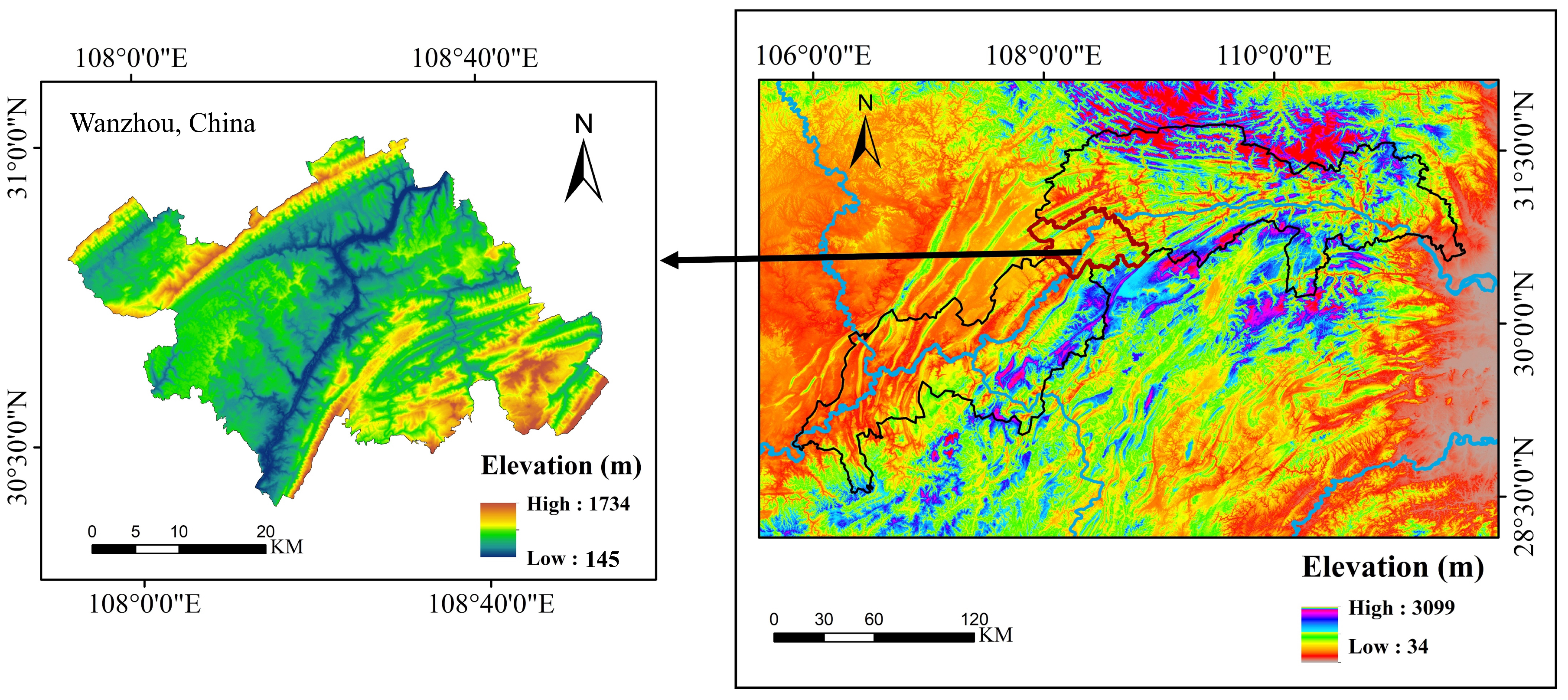
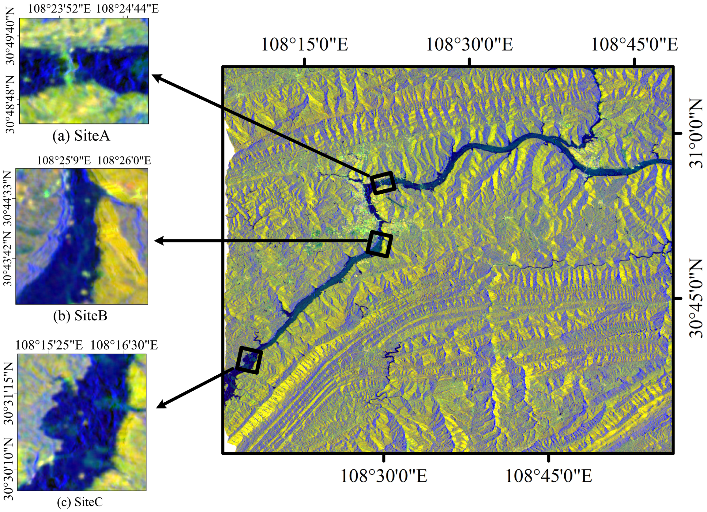
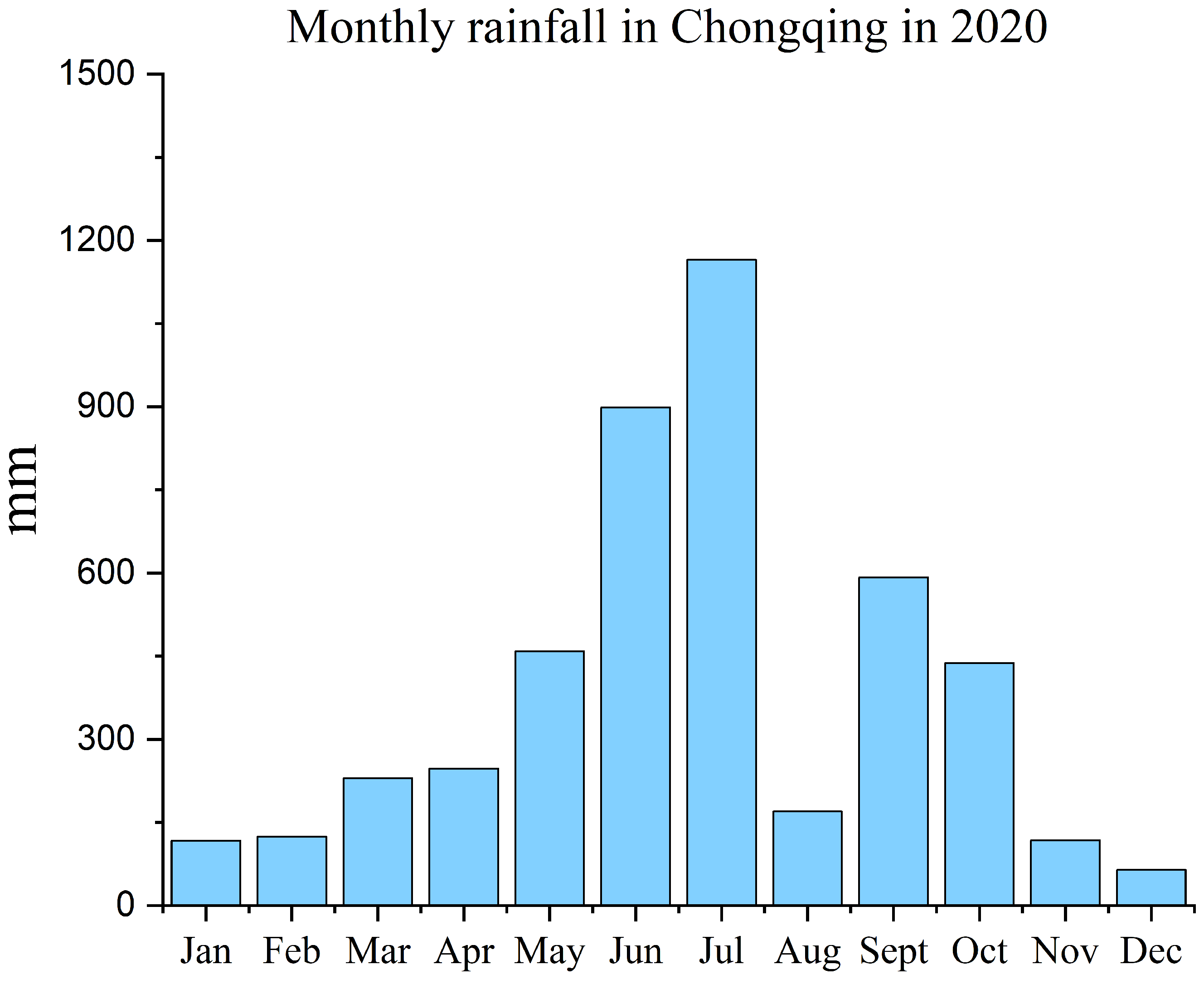
2.1.1. Study Area
2.1.2. Data
2.2. Methodology
2.2.1. Support Vector Machine
2.2.2. Extreme Gradient Boosting
2.2.3. Random Forest
2.2.4. Hyperparameters Optimization-Seeking Algorithms
- Construct an initial population (where each individual in the population represents a solution).
- Calculate the fitness of individuals in the population using an evaluation function.
- Use fitness values to calculate the probability of selecting individuals from the population.
- Generate the next generation of the population by combining different individuals through crossover.
- Introduce a certain mutation probability to randomly change some elements of individuals’ sequences to prevent becoming trapped in local optima.
- Iterate until termination conditions are met (e.g., reaching a maximum number of generations or satisfying convergence criteria).
2.2.5. Statistical Indicators
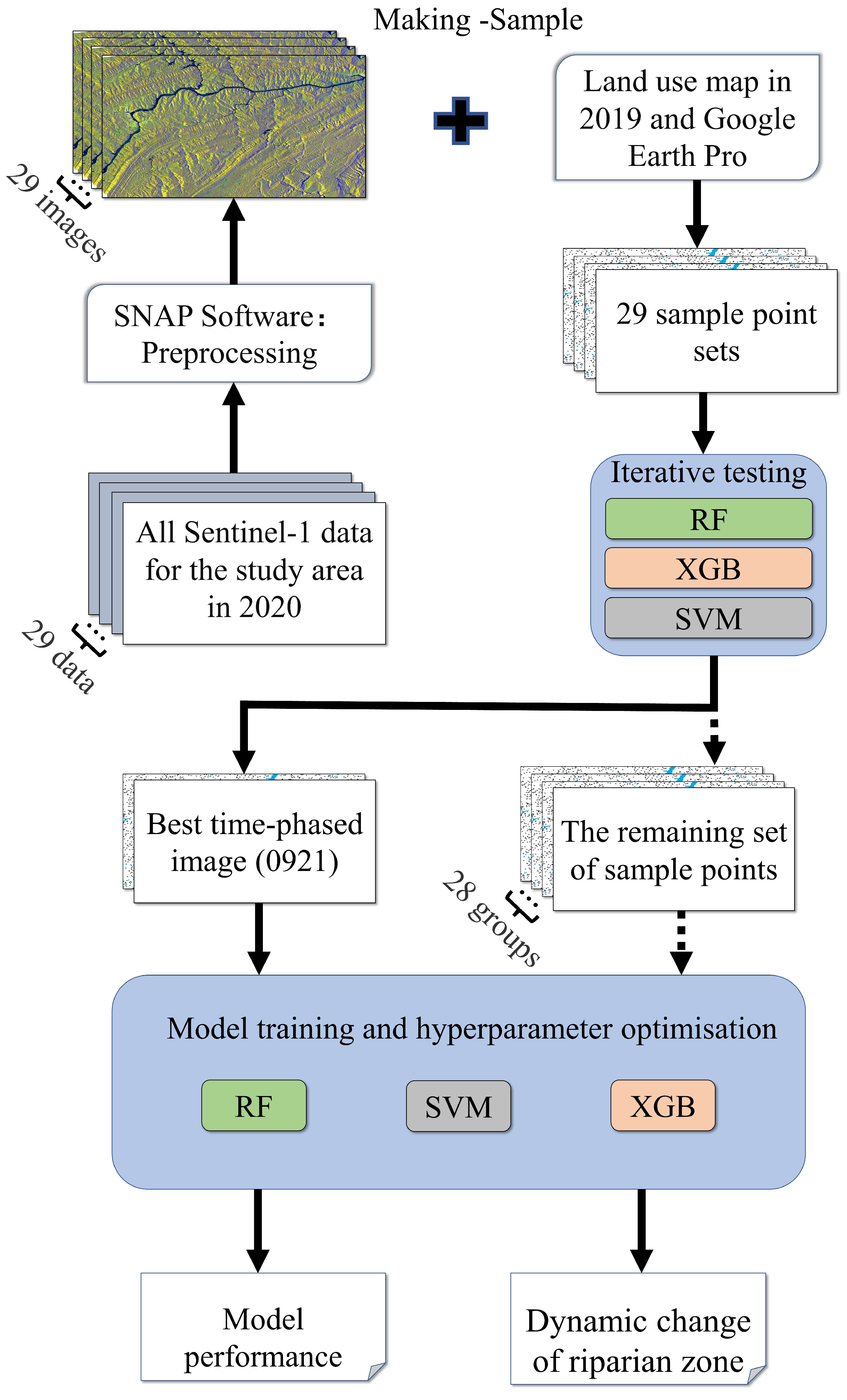
2.3. Overall Process
3. Results
3.1. Optimal Phase
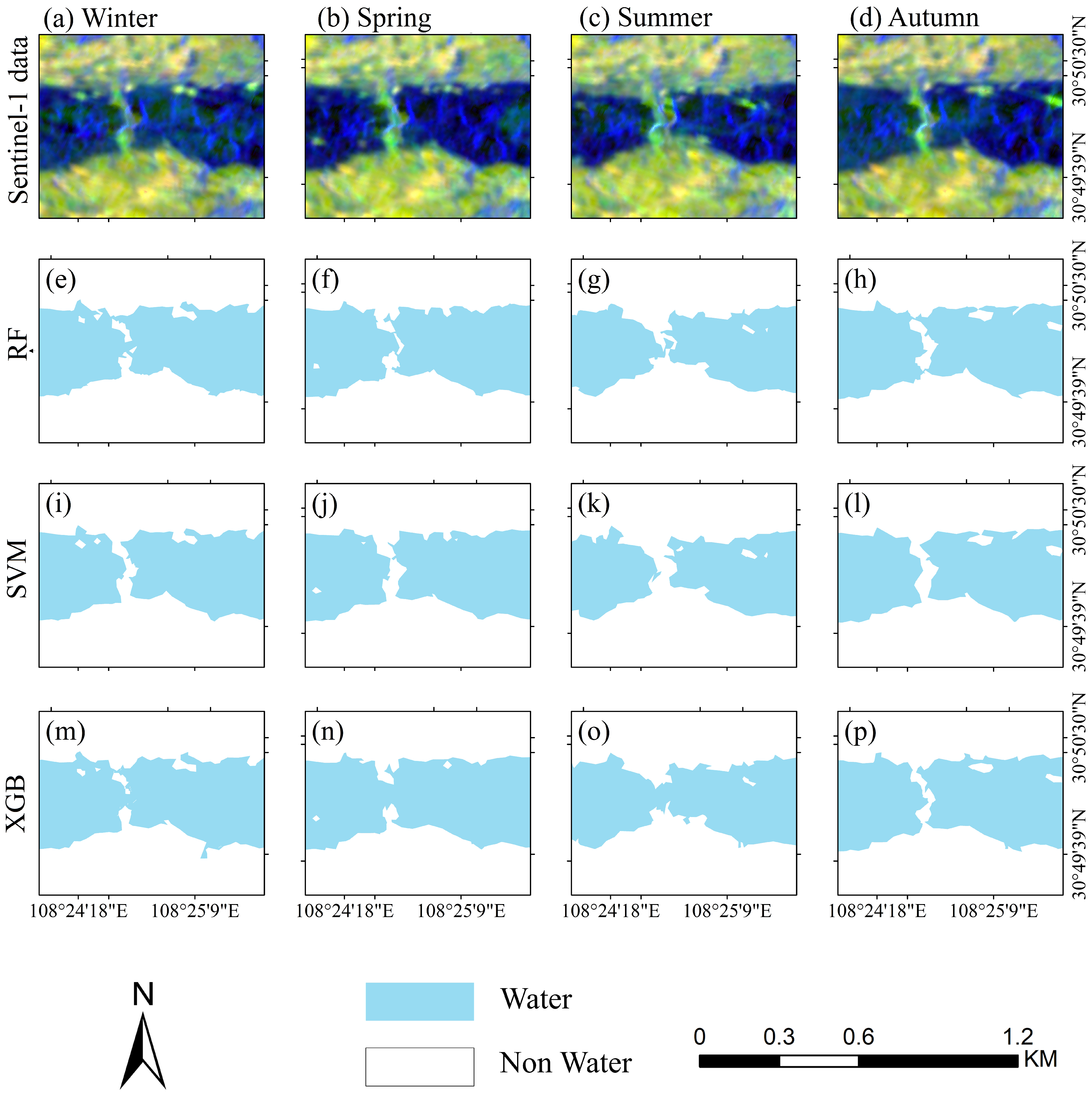
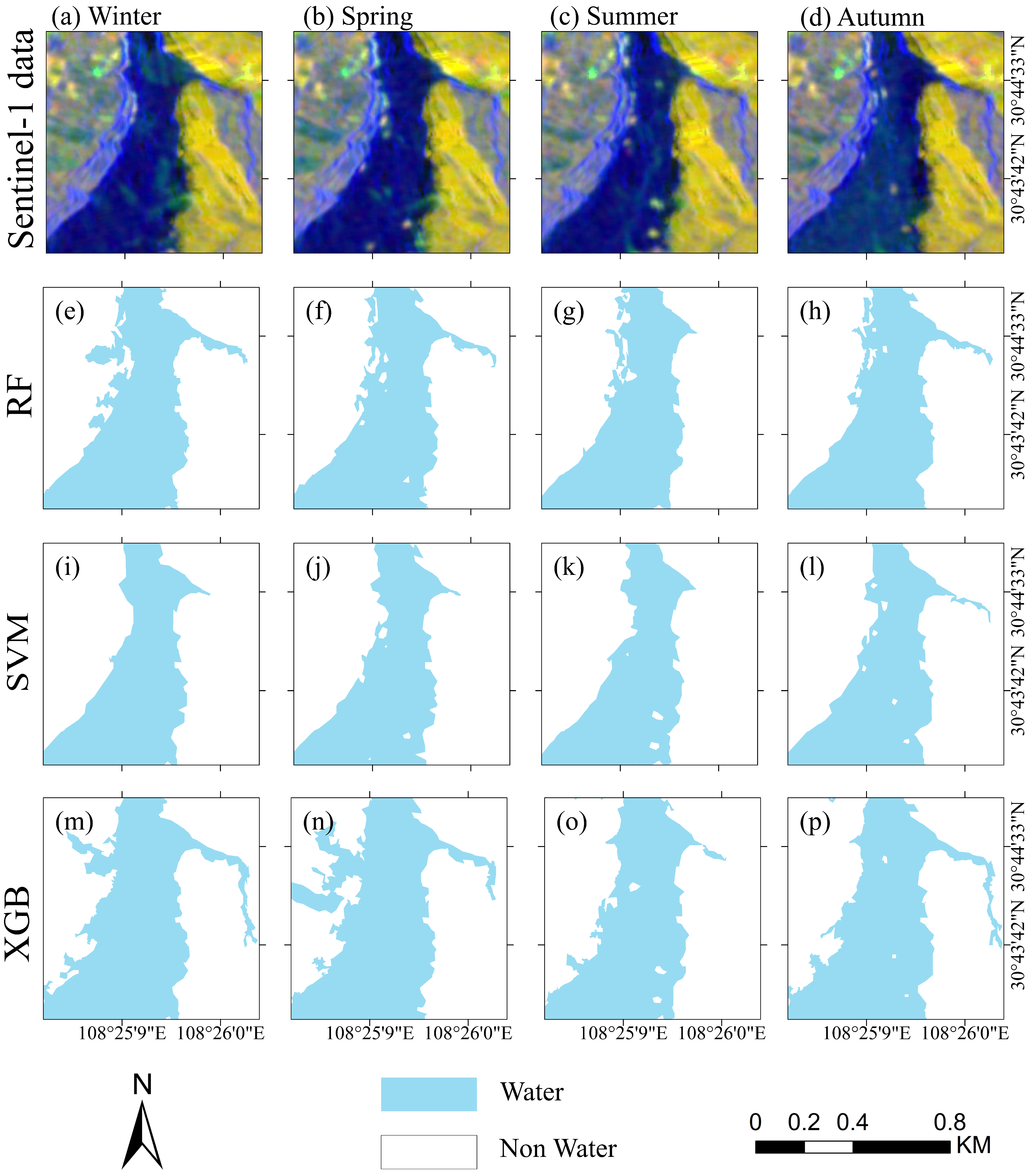
3.2. Identification of Surface with Optimal Models
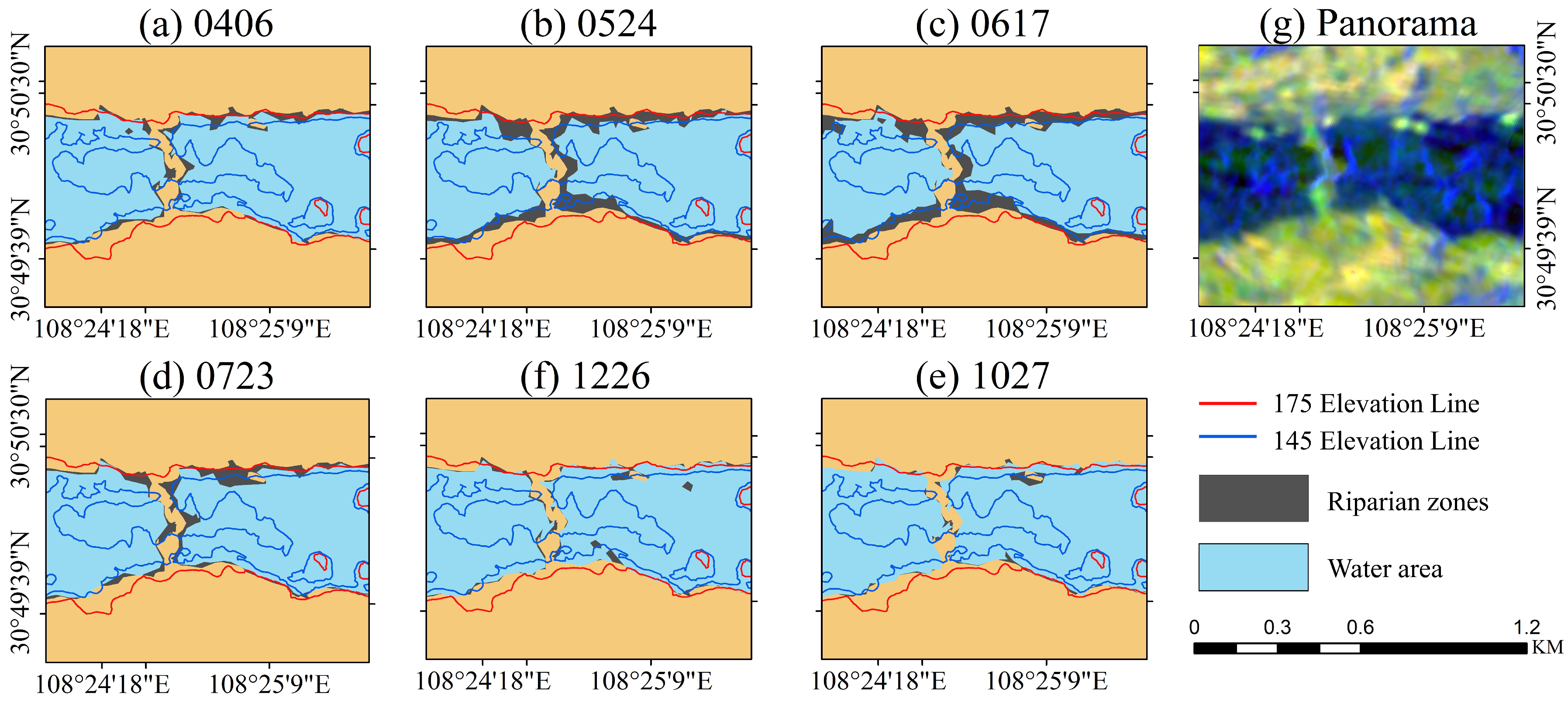
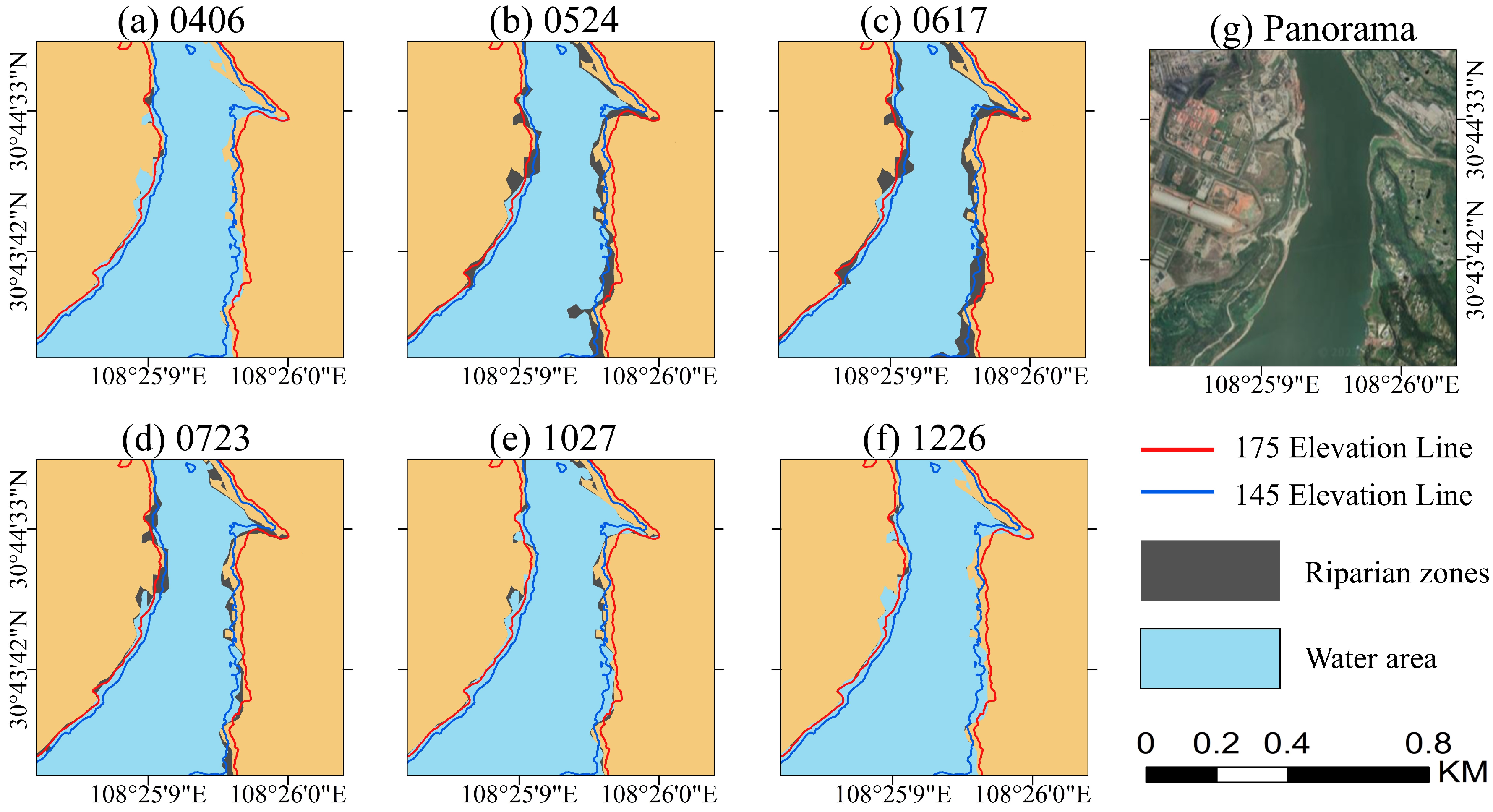
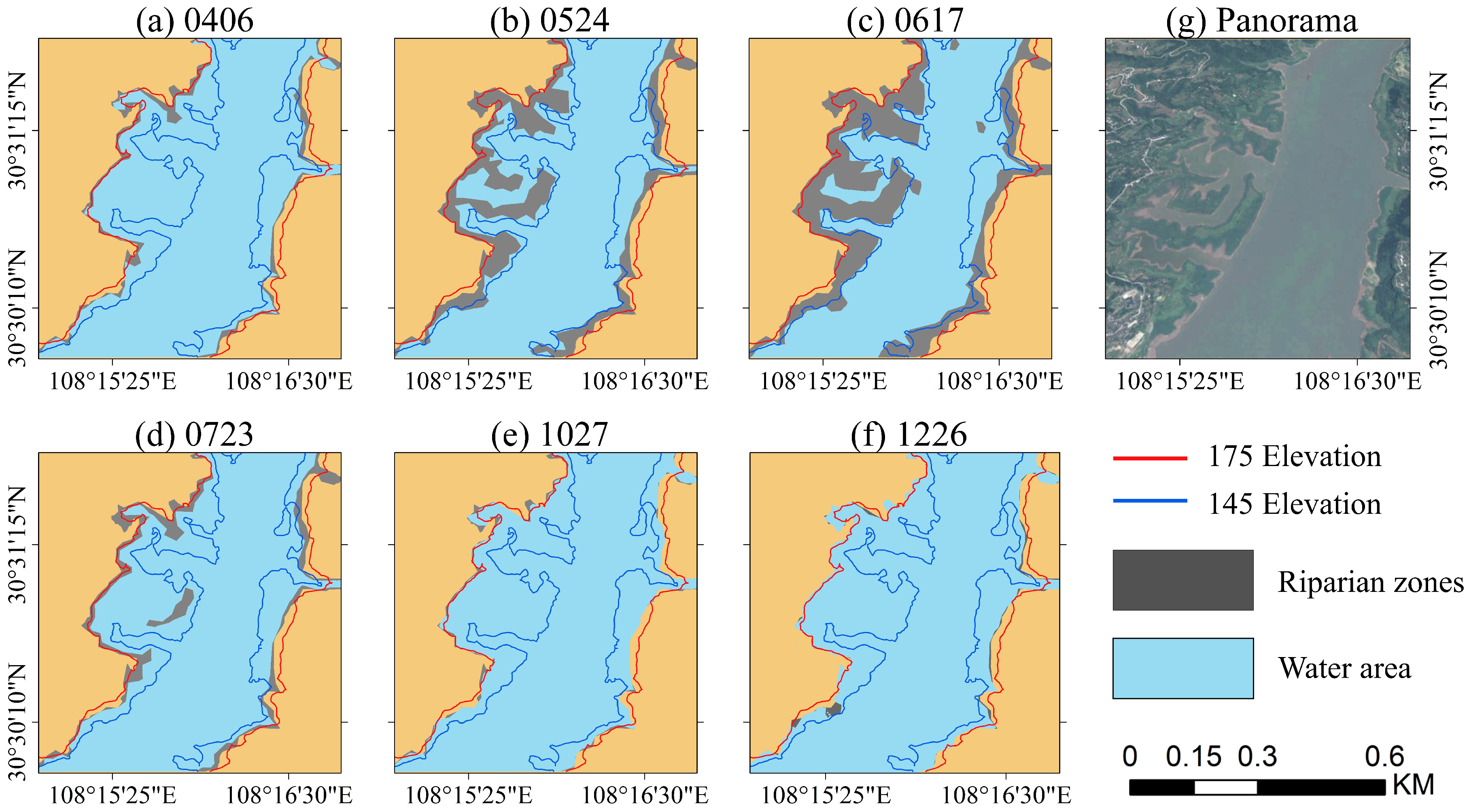
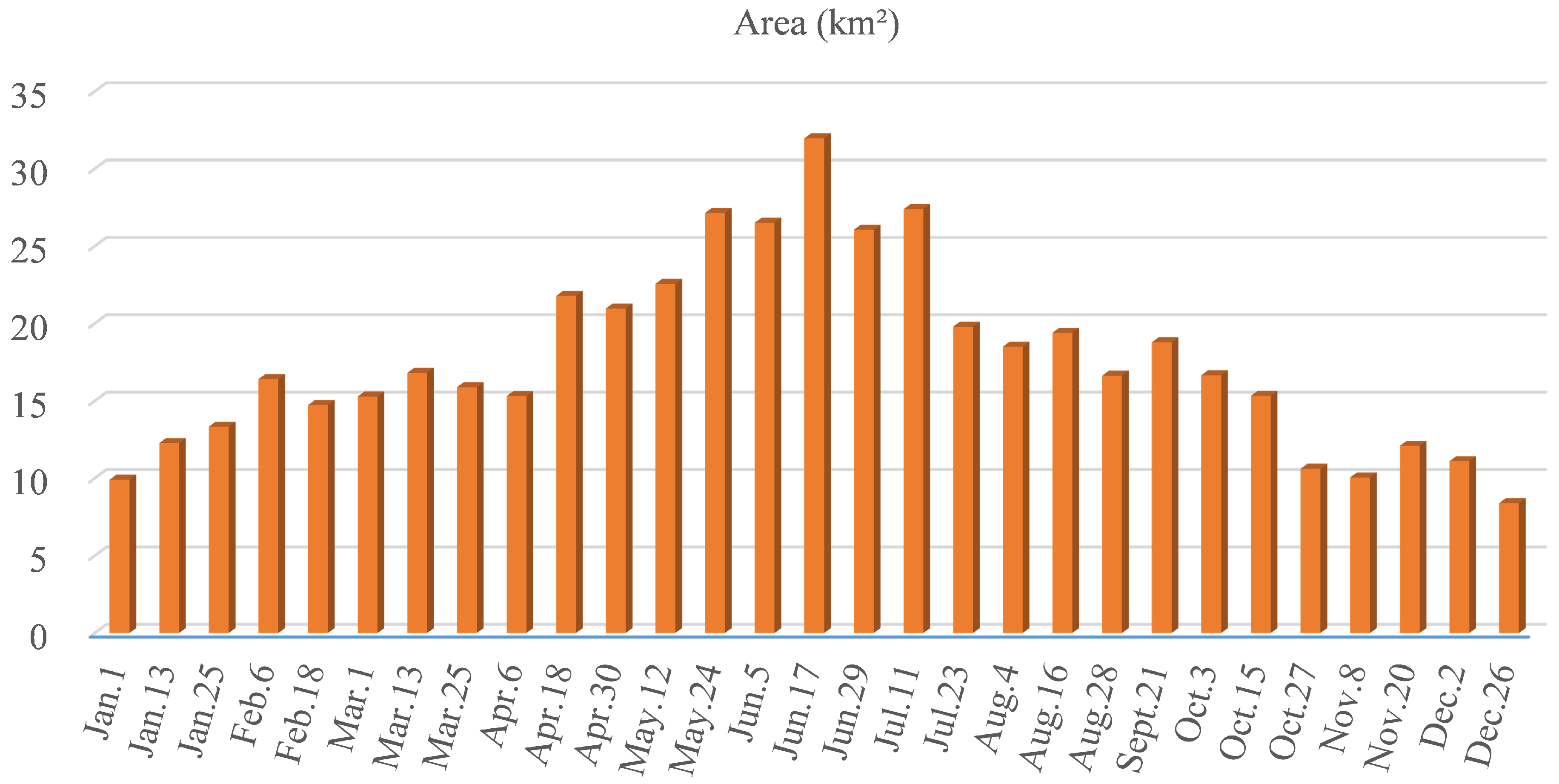
3.3. Surface Change in the Riparian Zone
4. Discussion
4.1. The Model Performance
4.2. The Area Change in the Riparian Zone
5. Conclusions
Author Contributions
Funding
Data Availability Statement
Conflicts of Interest
Appendix A

| Image | ACC | |||||
|---|---|---|---|---|---|---|
| RF | XGB | SVM | ||||
| Before GA | After GA | Before GA | After GA | Before GA | After GA | |
| 0125 | 0.929 | 0.94 | 0.9312 | 0.94 | 0.9231 | 0.9386 |
| 0325 | 0.9349 | 0.9438 | 0.9305 | 0.9424 | 0.9227 | 0.9434 |
| 0629 | 0.9206 | 0.9422 | 0.9223 | 0.9383 | 0.9217 | 0.9427 |
| 1226 | 0.9291 | 0.938 | 0.9326 | 0.9395 | 0.9321 | 0.9403 |
| Image | F1_score | |||||
| RF | XGB | SVM | ||||
| Before GA | After GA | Before GA | After GA | Before GA | After GA | |
| 0125 | 0.9332 | 0.9455 | 0.9397 | 0.9454 | 0.9399 | 0.9447 |
| 0325 | 0.9381 | 0.9479 | 0.9332 | 0.9456 | 0.9274 | 0.9489 |
| 0629 | 0.9227 | 0.9465 | 0.9315 | 0.9426 | 0.9226 | 0.9477 |
| 1226 | 0.9352 | 0.9464 | 0.9382 | 0.9434 | 0.9338 | 0.9464 |
| Image | Kappa | |||||
| RF | XGB | SVM | ||||
| Before GA | After GA | Before GA | After GA | Before GA | After GA | |
| 0125 | 0.8687 | 0.8791 | 0.8673 | 0.8792 | 0.8655 | 0.8762 |
| 0325 | 0.8763 | 0.8851 | 0.8754 | 0.8844 | 0.8631 | 0.886 |
| 0629 | 0.8621 | 0.8837 | 0.8647 | 0.8761 | 0.8645 | 0.8847 |
| 1226 | 0.8734 | 0.8841 | 0.8756 | 0.8803 | 0.8652 | 0.8796 |
| Image | Time (s) | ||||||||
|---|---|---|---|---|---|---|---|---|---|
| Optimization Time | Execution Time (After GA) | Execution Time (Default) | |||||||
| RF | XGB | SVM | RF | XGB | SVM | RF | XGB | SVM | |
| 0125 | 7114.6 | 7225 | 7072.1 | 594 | 603 | 585 | 597 | 599 | 579 |
| 0325 | 6974.1 | 6894.1 | 6768 | 589 | 594 | 587 | 583 | 585 | 589 |
| 0629 | 7214.5 | 7326.3 | 7095.1 | 592 | 594 | 593 | 597 | 599 | 591 |
| 1226 | 8744.7 | 8737.8 | 8667.2 | 593 | 592 | 593 | 586 | 593 | 590 |
Appendix B
References
- Jiao, L.; Zhang, Z.-N. Ecological Science A Summary of Water-Level-Fluctuating Zone. Ecol. Sci. 2013, 32, 259–264. [Google Scholar]
- Yin, D.; Wang, Y.; Jiang, T.; Qin, C.; Xiang, Y.; Chen, Q.; Xue, J.; Wang, D. Methylmercury production in soil in the water-level-fluctuating zone of the Three Gorges Reservoir, China: The key role of low-molecular-weight organic acids. Environ. Pollut. 2018, 235, 186–196. [Google Scholar] [CrossRef] [PubMed]
- Chen, Z.; Yuan, X.; Roß-Nickoll, M.; Hollert, H.; Schäffer, A. Moderate inundation stimulates plant community assembly in the drawdown zone of China’s Three Gorges Reservoir. Environ. Sci. Eur. 2020, 32, 79. [Google Scholar] [CrossRef]
- Tangen, B.A.; Bansal, S. Hydrologic lag effects on wetland greenhouse gas fluxes. Atmosphere 2019, 10, 269. [Google Scholar] [CrossRef]
- Gownaris, N.J.; Pikitch, E.K.; Aller, J.Y.; Kaufman, L.S.; Kolding, J.; Lwiza, K.M.; Obiero, K.O.; Ojwang, W.O.; Malala, J.O.; Rountos, K.J. Fisheries and water level fluctuations in the world’s largest desert lake. Ecohydrology 2017, 10, e1769. [Google Scholar] [CrossRef]
- Naiman, R.J.; Decamps, H. The ecology of interfaces: Riparian zones. Annu. Rev. Ecol. Syst. 1997, 28, 621–658. [Google Scholar] [CrossRef]
- Aguiar, F.C.; Fernandes, M.R.; Ferreira, M.T. Riparian vegetation metrics as tools for guiding ecological restoration in riverscapes. Knowl. Manag. Aquat. Ecosyst. 2011, 402, 21. [Google Scholar] [CrossRef]
- Tian, Y.; Guo, Z.; Zhong, W.; Qiao, Y.; Qin, J. A design of ecological restoration and eco-revetment construction for the riparian zone of Xianghe Segment of China’s Grand Canal. Int. J. Sustain. Dev. World Ecol. 2016, 23, 333–342. [Google Scholar] [CrossRef]
- Olokeogun, O.S.; Ayanlade, A.; Popoola, O.O. Assessment of riparian zone dynamics and its flood-related implications in Eleyele area of Ibadan, Nigeria. Environ. Syst. Res. 2020, 9, 6. [Google Scholar] [CrossRef]
- Dempsey, J.A.; Plantinga, A.J.; Kline, J.D.; Lawler, J.J.; Martinuzzi, S.; Radeloff, V.C.; Bigelow, D.P. Effects of local land-use planning on development and disturbance in riparian areas. Land Use Policy 2017, 60, 16–25. [Google Scholar] [CrossRef]
- Du, C.; Li, Y.; Wang, Q.; Liu, G.; Zheng, Z.; Mu, M.; Li, Y. Tempo-spatial dynamics of water quality and its response to river flow in estuary of Taihu Lake based on GOCI imagery. Environ. Sci. Pollut. Res. 2017, 24, 28079–28101. [Google Scholar] [CrossRef]
- de Bruijn, J.A.; de Moel, H.; Jongman, B.; de Ruiter, M.C.; Wagemaker, J.; Aerts, J.C. A global database of historic and real-time flood events based on social media. Sci. Data 2019, 6, 311. [Google Scholar] [CrossRef]
- Goldberg, M.D.; Li, S.; Goodman, S.; Lindsey, D.; Sjoberg, B.; Sun, D. Contributions of operational satellites in monitoring the catastrophic floodwaters due to Hurricane Harvey. Remote Sens. 2018, 10, 1256. [Google Scholar] [CrossRef]
- Demirkesen, A.; Evrendilek, F.; Berberoglu, S.; Kilic, S. Coastal flood risk analysis using Landsat-7 ETM+ imagery and SRTM DEM: A case study of Izmir, Turkey. Environ. Monit. Assess. 2007, 131, 293–300. [Google Scholar] [CrossRef] [PubMed]
- Radočaj, D.; Obhođaš, J.; Jurišić, M.; Gašparović, M. Global open data remote sensing satellite missions for land monitoring and conservation: A review. Land 2020, 9, 402. [Google Scholar] [CrossRef]
- Phiri, D.; Simwanda, M.; Salekin, S.; Nyirenda, V.R.; Murayama, Y.; Ranagalage, M. Sentinel-2 data for land cover/use mapping: A review. Remote Sens. 2020, 12, 2291. [Google Scholar] [CrossRef]
- Adeli, S.; Salehi, B.; Mahdianpari, M.; Quackenbush, L.J.; Brisco, B.; Tamiminia, H.; Shaw, S. Wetland monitoring using SAR data: A meta-analysis and comprehensive review. Remote Sens. 2020, 12, 2190. [Google Scholar] [CrossRef]
- Cazals, C.; Rapinel, S.; Frison, P.L.; Bonis, A.; Mercier, G.; Mallet, C.; Corgne, S.; Rudant, J.P. Mapping and characterization of hydrological dynamics in a coastal marsh using high temporal resolution Sentinel-1A images. Remote Sens. 2016, 8, 570. [Google Scholar] [CrossRef]
- Vasco, D.W.; Kim, K.H.; Farr, T.G.; Reager, J.; Bekaert, D.; Sangha, S.S.; Rutqvist, J.; Beaudoing, H.K. Using Sentinel-1 and GRACE satellite data to monitor the hydrological variations within the Tulare Basin, California. Sci. Rep. 2022, 12, 3867. [Google Scholar] [CrossRef]
- Berger, M.; Moreno, J.; Johannessen, J.A.; Levelt, P.F.; Hanssen, R.F. ESA’s sentinel missions in support of Earth system science. Remote. Sens. Environ. 2012, 120, 84–90. [Google Scholar] [CrossRef]
- Guzder-Williams, B.; Alemohammad, H. Surface Water Detection from Sentinel-1. In Proceedings of the 2021 IEEE International Geoscience and Remote Sensing Symposium IGARSS, Virtual, 12–16 July 2021; pp. 286–289. [Google Scholar] [CrossRef]
- Martinis, S.; Plank, S.; Ćwik, K. The use of Sentinel-1 time-series data to improve flood monitoring in arid areas. Remote Sens. 2018, 10, 583. [Google Scholar] [CrossRef]
- Souza, W.d.O.; Reis, L.G.d.M.; Ruiz-Armenteros, A.M.; Veleda, D.; Ribeiro Neto, A.; Fragoso Jr, C.R.; Cabral, J.J.d.S.P.; Montenegro, S.M.G.L. Analysis of environmental and atmospheric influences in the use of sar and optical imagery from sentinel-1, landsat-8, and sentinel-2 in the operational monitoring of reservoir water level. Remote Sens. 2022, 14, 2218. [Google Scholar] [CrossRef]
- Carreño Conde, F.; De Mata Muñoz, M. Flood monitoring based on the study of Sentinel-1 SAR images: The Ebro River case study. Water 2019, 11, 2454. [Google Scholar] [CrossRef]
- Lee, J.S. Refined filtering of image noise using local statistics. Comput. Graph. Image Process. 1981, 15, 380–389. [Google Scholar] [CrossRef]
- Moghimi, A.; Khazai, S.; Mohammadzadeh, A. An improved fast level set method initialized with a combination of k-means clustering and Otsu thresholding for unsupervised change detection from SAR images. Arab. J. Geosci. 2017, 10, 293. [Google Scholar] [CrossRef]
- Moghimi, A.; Mohammadzadeh, A.; Khazai, S. Integrating thresholding with level set method for unsupervised change detection in multitemporal SAR images. Can. J. Remote Sens. 2017, 43, 412–431. [Google Scholar] [CrossRef]
- Vickers, H.; Malnes, E.; Høgda, K.A. Long-term water surface area monitoring and derived water level using synthetic aperture radar (SAR) at altevatn, a medium-sized arctic lake. Remote Sens. 2019, 11, 2780. [Google Scholar] [CrossRef]
- Hardy, A.; Ettritch, G.; Cross, D.E.; Bunting, P.; Liywalii, F.; Sakala, J.; Silumesii, A.; Singini, D.; Smith, M.; Willis, T.; et al. Automatic detection of open and vegetated water bodies using Sentinel 1 to map African malaria vector mosquito breeding habitats. Remote Sens. 2019, 11, 593. [Google Scholar] [CrossRef]
- Nickmilder, C.; Tedde, A.; Dufrasne, I.; Lessire, F.; Tychon, B.; Curnel, Y.; Bindelle, J.; Soyeurt, H. Development of machine learning models to predict compressed sward height in Walloon pastures based on Sentinel-1, Sentinel-2 and meteorological data using multiple data transformations. Remote Sens. 2021, 13, 408. [Google Scholar] [CrossRef]
- Slagter, B.; Tsendbazar, N.E.; Vollrath, A.; Reiche, J. Mapping wetland characteristics using temporally dense Sentinel-1 and Sentinel-2 data: A case study in the St. Lucia wetlands, South Africa. Int. J. Appl. Earth Obs. Geoinf. 2020, 86, 102009. [Google Scholar] [CrossRef]
- Acharya, T.D.; Subedi, A.; Lee, D.H. Evaluation of machine learning algorithms for surface water extraction in a Landsat 8 scene of Nepal. Sensors 2019, 19, 2769. [Google Scholar] [CrossRef] [PubMed]
- Luo, J.; Chen, Z.; Chen, N. Distinguishing different subclasses of water bodies for long-term and large-scale statistics of lakes: A case study of the Yangtze River basin from 2008 to 2018. Int. J. Digit. Earth 2021, 14, 202–230. [Google Scholar] [CrossRef]
- Anderssen, R.; Bloomfield, P. Properties of the random search in global optimization. J. Optim. Theory Appl. 1975, 16, 383–398. [Google Scholar] [CrossRef]
- Herrera, F.; Lozano, M.; Verdegay, J.L. Tackling real-coded genetic algorithms: Operators and tools for behavioural analysis. Artif. Intell. Rev. 1998, 12, 265–319. [Google Scholar] [CrossRef]
- Žilinskas, A.; Zhigljavsky, A. Stochastic global optimization: A review on the occasion of 25 years of Informatica. Informatica 2016, 27, 229–256. [Google Scholar] [CrossRef]
- Xie, Y.; Li, P.; Zhang, J.; Ogiela, M.R. Differential privacy distributed learning under chaotic quantum particle swarm optimization. Computing 2021, 103, 449–472. [Google Scholar] [CrossRef]
- Tani, L.; Rand, D.; Veelken, C.; Kadastik, M. Evolutionary algorithms for hyperparameter optimization in machine learning for application in high energy physics. Eur. Phys. J. C 2021, 81, 1–9. [Google Scholar] [CrossRef]
- Huang, M.; Gong, J.; Shi, Z.; Liu, C.; Zhang, L. Genetic algorithm-based decision tree classifier for remote sensing mapping with SPOT-5 data in the HongShiMao watershed of the loess plateau, China. Neural Comput. Appl. 2007, 16, 513–517. [Google Scholar] [CrossRef]
- Sorkhabi, O.M.; Shadmanfar, B.; Kiani, E. Monitoring of dam reservoir storage with multiple satellite sensors and artificial intelligence. Results Eng. 2022, 16, 100542. [Google Scholar] [CrossRef]
- Bouktif, S.; Fiaz, A.; Ouni, A.; Serhani, M.A. Optimal deep learning lstm model for electric load forecasting using feature selection and genetic algorithm: Comparison with machine learning approaches. Energies 2018, 11, 1636. [Google Scholar] [CrossRef]
- Toma, R.N.; Prosvirin, A.E.; Kim, J.M. Bearing fault diagnosis of induction motors using a genetic algorithm and machine learning classifiers. Sensors 2020, 20, 1884. [Google Scholar] [CrossRef]
- Shao, Y.; Lin, J.C.W.; Srivastava, G.; Guo, D.; Zhang, H.; Yi, H.; Jolfaei, A. Multi-objective neural evolutionary algorithm for combinatorial optimization problems. IEEE Trans. Neural Netw. Learn. Syst. 2021, 34, 2133–2143. [Google Scholar] [CrossRef]
- Cortes, C.; Vapnik, V. Support-vector networks. Mach. Learn. 1995, 20, 273–297. [Google Scholar] [CrossRef]
- Sheykhmousa, M.; Mahdianpari, M.; Ghanbari, H.; Mohammadimanesh, F.; Ghamisi, P.; Homayouni, S. Support vector machine versus random forest for remote sensing image classification: A meta-analysis and systematic review. IEEE J. Sel. Top. Appl. Earth Obs. Remote Sens. 2020, 13, 6308–6325. [Google Scholar] [CrossRef]
- Chen, T.; Guestrin, C. Xgboost: A scalable tree boosting system. In Proceedings of the 22nd acm SIGKDD International Conference on Knowledge Discovery and Data Mining, San Francisco, CA, USA, 13–17 August 2016; pp. 785–794. [Google Scholar]
- Zhang, H.; Eziz, A.; Xiao, J.; Tao, S.; Wang, S.; Tang, Z.; Zhu, J.; Fang, J. High-resolution vegetation mapping using eXtreme gradient boosting based on extensive features. Remote Sens. 2019, 11, 1505. [Google Scholar] [CrossRef]
- Breiman, L. Random forests. Mach. Learn. 2001, 45, 5–32. [Google Scholar] [CrossRef]
- Belgiu, M.; Drăguţ, L. Random forest in remote sensing: A review of applications and future directions. ISPRS J. Photogramm. Remote Sens. 2016, 114, 24–31. [Google Scholar] [CrossRef]
- Probst, P.; Wright, M.N.; Boulesteix, A.L. Hyperparameters and tuning strategies for random forest. Wiley Interdiscip. Rev. Data Min. Knowl. Discov. 2019, 9, e1301. [Google Scholar] [CrossRef]
- LaValle, S.M.; Branicky, M.S.; Lindemann, S.R. On the relationship between classical grid search and probabilistic roadmaps. Int. J. Robot. Res. 2004, 23, 673–692. [Google Scholar] [CrossRef]
- Jiang, J.J.; Wei, W.X.; Shao, W.L.; Liang, Y.F.; Qu, Y.Y. Research on large-scale bi-level particle swarm optimization algorithm. IEEE Access 2021, 9, 56364–56375. [Google Scholar] [CrossRef]
- Katoch, S.; Chauhan, S.S.; Kumar, V. A review on genetic algorithm: Past, present, and future. Multimed. Tools Appl. 2021, 80, 8091–8126. [Google Scholar] [CrossRef] [PubMed]
- Li, X.; Zheng, H.; Han, C.; Wang, H.; Dong, K.; Jing, Y.; Zheng, W. Cloud detection of superview-1 remote sensing images based on genetic reinforcement learning. Remote Sens. 2020, 12, 3190. [Google Scholar] [CrossRef]
- Paterna, S.; Santoni, M.; Bruzzone, L. An approach based on multiobjective genetic algorithms to schedule observations in planetary remote sensing missions. IEEE J. Sel. Top. Appl. Earth Obs. Remote Sens. 2020, 13, 4714–4727. [Google Scholar] [CrossRef]
- Chetty, S.; Adewumi, A.O. Three new stochastic local search algorithms for continuous optimization problems. Comput. Optim. Appl. 2013, 56, 675–721. [Google Scholar] [CrossRef]
- Wang, M.; Wan, Y.; Ye, Z.; Lai, X. Remote sensing image classification based on the optimal support vector machine and modified binary coded ant colony optimization algorithm. Inf. Sci. 2017, 402, 50–68. [Google Scholar] [CrossRef]
- Goutte, C.; Gaussier, E. A probabilistic interpretation of precision, recall and F-score, with implication for evaluation. In Proceedings of the European Conference on Information Retrieval, Santiago de Compostela, Spain, 21–23 March 2005; Springer: Berlin/Heidelberg, Germany, 2005; pp. 345–359. [Google Scholar]
- Ghaddar, B.; Naoum-Sawaya, J. High dimensional data classification and feature selection using support vector machines. Eur. J. Oper. Res. 2018, 265, 993–1004. [Google Scholar] [CrossRef]
- Xiang, D.; Zhang, X.; Wu, W.; Liu, H. Denseppmunet-a: A robust deep learning network for segmenting water bodies from aerial images. IEEE Trans. Geosci. Remote Sens. 2023, 61, 1–11. [Google Scholar] [CrossRef]

| Date | Code * | Date | Code * | Date | Code * | Date | Code * | Date | Code * |
|---|---|---|---|---|---|---|---|---|---|
| 1 January | 0101 | 13 March | 0313 | 24 May | 0524 | 4 August | 0804 | 27 October | 1027 |
| 13 January | 0113 | 25 March | 0325 | 5 June | 0605 | 16 August | 0816 | 8 November | 1108 |
| 25 January | 0125 | 6 April | 0406 | 17 June | 0617 | 28 August | 0828 | 20 November | 1120 |
| 6 February | 0206 | 18 April | 0418 | 29 June | 0629 | 21 September | 0921 | 2 December | 1202 |
| 18 February | 0218 | 30 April | 0430 | 11 July | 0711 | 3 October | 1003 | 26 December | 1226 |
| 1 March | 0301 | 12 May | 0512 | 23 July | 0723 | 15 October | 1015 |
| Classifier | Hyperparameter | Candidate Value | Combination Number | Optimization Result |
|---|---|---|---|---|
| SVM | c | 0.01–1000 | 2.56 × | 15.886 |
| gamma | 0.0001–256 | 0.0039 | ||
| RF | max_depth | 1–600 | 6 × | 256 |
| n_estimators | 1–1000 | 997 | ||
| XGB | learning_rate | 0.01–1.0 | 0.104 | |
| sub_sample | 0.01–1.0 | 0.772 |
| Prediction | |||
|---|---|---|---|
| Positive (Pos) | Negative (Neg) | ||
| Ground truth | Positive | TP (True Pos) | FN (False Neg) |
| Negative | FP (False Pos) | TN (True Neg) | |
| Image | ACC | F1_score | Kappa | ||||||
|---|---|---|---|---|---|---|---|---|---|
| RF | XGB | SVM | RF | XGB | SVM | RF | XGB | SVM | |
| 0101 | 0.9406 | 0.9411 | 0.9395 | 0.9465 | 0.9457 | 0.9456 | 0.8803 | 0.8812 | 0.8779 |
| 0113 | 0.9416 | 0.9403 | 0.9400 | 0.9471 | 0.9458 | 0.9460 | 0.8824 | 0.8796 | 0.8790 |
| 0125 | 0.9400 | 0.9400 | 0.9386 | 0.9455 | 0.9454 | 0.9447 | 0.8791 | 0.8792 | 0.8762 |
| 0206 | 0.9410 | 0.9370 | 0.9451 | 0.9449 | 0.9399 | 0.9501 | 0.8815 | 0.8736 | 0.8894 |
| 0218 | 0.9433 | 0.9432 | 0.9402 | 0.9476 | 0.9446 | 0.9460 | 0.8859 | 0.8840 | 0.8794 |
| 0301 | 0.9435 | 0.9431 | 0.9437 | 0.9465 | 0.9463 | 0.9490 | 0.8845 | 0.8849 | 0.8866 |
| 0313 | 0.9410 | 0.9344 | 0.9424 | 0.9445 | 0.9365 | 0.9479 | 0.8815 | 0.8686 | 0.8839 |
| 0325 | 0.9438 | 0.9424 | 0.9434 | 0.9479 | 0.9456 | 0.9489 | 0.8851 | 0.8844 | 0.8860 |
| 0406 | 0.9424 | 0.9423 | 0.9436 | 0.9452 | 0.9454 | 0.9490 | 0.8831 | 0.8841 | 0.8862 |
| 0418 | 0.9406 | 0.9383 | 0.9445 | 0.9443 | 0.9412 | 0.9491 | 0.8807 | 0.8762 | 0.8882 |
| 0430 | 0.9433 | 0.9388 | 0.9451 | 0.9473 | 0.9419 | 0.9503 | 0.8860 | 0.8772 | 0.8894 |
| 0512 | 0.9430 | 0.9431 | 0.9412 | 0.9462 | 0.9450 | 0.9470 | 0.8853 | 0.8850 | 0.8814 |
| 0524 | 0.9381 | 0.9320 | 0.9415 | 0.9422 | 0.9355 | 0.9462 | 0.8756 | 0.8636 | 0.8823 |
| 0605 | 0.9250 | 0.9240 | 0.9327 | 0.9309 | 0.9289 | 0.9392 | 0.8492 | 0.8474 | 0.8642 |
| 0617 | 0.9234 | 0.9172 | 0.9338 | 0.9260 | 0.9189 | 0.9376 | 0.8465 | 0.8343 | 0.8671 |
| 0629 | 0.9422 | 0.9383 | 0.9427 | 0.9465 | 0.9426 | 0.9477 | 0.8837 | 0.8761 | 0.8847 |
| 0711 | 0.9372 | 0.9345 | 0.9414 | 0.9410 | 0.9382 | 0.9460 | 0.8738 | 0.8686 | 0.8822 |
| 0723 | 0.9368 | 0.9339 | 0.9406 | 0.9414 | 0.9384 | 0.9457 | 0.8729 | 0.8672 | 0.8803 |
| 0804 | 0.9431 | 0.9407 | 0.9421 | 0.9479 | 0.9454 | 0.9475 | 0.8855 | 0.8807 | 0.8834 |
| 0816 | 0.9433 | 0.9391 | 0.9445 | 0.9472 | 0.9420 | 0.9494 | 0.8861 | 0.8779 | 0.8882 |
| 0828 | 0.9400 | 0.9361 | 0.9438 | 0.9435 | 0.9383 | 0.9488 | 0.8795 | 0.8720 | 0.8869 |
| 0921 | 0.9435 | 0.9437 | 0.9454 | 0.9475 | 0.9459 | 0.9504 | 0.8864 | 0.8850 | 0.8899 |
| 1003 | 0.9370 | 0.9329 | 0.9399 | 0.9410 | 0.9363 | 0.9444 | 0.8735 | 0.8654 | 0.8791 |
| 1015 | 0.9281 | 0.9191 | 0.9411 | 0.9308 | 0.9201 | 0.9454 | 0.8560 | 0.8382 | 0.8816 |
| 1027 | 0.9413 | 0.9411 | 0.9439 | 0.9454 | 0.9441 | 0.9492 | 0.8821 | 0.8819 | 0.8869 |
| 1108 | 0.9402 | 0.9382 | 0.9405 | 0.9452 | 0.9411 | 0.9464 | 0.8824 | 0.8762 | 0.8800 |
| 1120 | 0.9377 | 0.9386 | 0.9387 | 0.9435 | 0.9413 | 0.9445 | 0.8789 | 0.8770 | 0.8758 |
| 1202 | 0.9415 | 0.9422 | 0.9432 | 0.9465 | 0.9437 | 0.9486 | 0.8851 | 0.8806 | 0.8856 |
| 1226 | 0.9380 | 0.9395 | 0.9403 | 0.9464 | 0.9434 | 0.9464 | 0.8841 | 0.8803 | 0.8796 |
Disclaimer/Publisher’s Note: The statements, opinions and data contained in all publications are solely those of the individual author(s) and contributor(s) and not of MDPI and/or the editor(s). MDPI and/or the editor(s) disclaim responsibility for any injury to people or property resulting from any ideas, methods, instructions or products referred to in the content. |
© 2023 by the authors. Licensee MDPI, Basel, Switzerland. This article is an open access article distributed under the terms and conditions of the Creative Commons Attribution (CC BY) license (https://creativecommons.org/licenses/by/4.0/).
Share and Cite
Xu, B.; Wu, W.; Ye, H.; Li, X.; Liu, H. Monitoring the Area Change in the Three Gorges Reservoir Riparian Zone Based on Genetic Algorithm Optimized Machine Learning Algorithms and Sentinel-1 Data. Remote Sens. 2023, 15, 5456. https://doi.org/10.3390/rs15235456
Xu B, Wu W, Ye H, Li X, Liu H. Monitoring the Area Change in the Three Gorges Reservoir Riparian Zone Based on Genetic Algorithm Optimized Machine Learning Algorithms and Sentinel-1 Data. Remote Sensing. 2023; 15(23):5456. https://doi.org/10.3390/rs15235456
Chicago/Turabian StyleXu, Baisheng, Wei Wu, Haohui Ye, Xinrong Li, and Hongbin Liu. 2023. "Monitoring the Area Change in the Three Gorges Reservoir Riparian Zone Based on Genetic Algorithm Optimized Machine Learning Algorithms and Sentinel-1 Data" Remote Sensing 15, no. 23: 5456. https://doi.org/10.3390/rs15235456
APA StyleXu, B., Wu, W., Ye, H., Li, X., & Liu, H. (2023). Monitoring the Area Change in the Three Gorges Reservoir Riparian Zone Based on Genetic Algorithm Optimized Machine Learning Algorithms and Sentinel-1 Data. Remote Sensing, 15(23), 5456. https://doi.org/10.3390/rs15235456