Sentinel-1 Imagery Used for Estimation of Soil Organic Carbon by Dual-Polarization SAR Vegetation Indices

Abstract

Despite optical remote sensing (and the spectral vegetation indices) contributions to digital soil-mapping studies of soil organic carbon (SOC), few studies have used active radar remote sensing mission data like that from synthetic aperture radar (SAR) sensors to predict SOC. Bearing in mind the importance of SOC mapping for agricultural, ecological, and climate interests and also the recently developed methods for vegetation monitoring using Sentinel-1 SAR data, in this work, we aimed to take advantage of the high operationality of Sentinel-1 imaging to test the accuracy of SOC prediction at different soil depths using machine learning systems. Using linear, nonlinear, and tree regression-based methods, it was possible to predict the SOC content of soils from western Bahia, Brazil, a region with predominantly sandy soils, using as explanatory variables the SAR vegetation indices. The models fed with SAR sensor polarizations and vegetation indices produced more accurate results for the topsoil layers (0–5 cm and 5–10 cm in depth). In these superficial layers, the models achieved an RMSE in the order of 5.0 g kg⁻¹ and an R² ranging from 0.16 to 0.24, therefore explaining about 20% of SOC variability using only Sentinel-1 predictors.

1. Introduction

Soil organic carbon (SOC) plays an important role in several ecological and agricultural processes related to physical, chemical, biological, and soil fertility properties and the biogeochemical carbon cycle in the Earth system [1]. Unfrozen soils are the third carbon pool in the Earth system [2] in the mineralized form (CaCO₃) and mainly in the organic form (SOC). Given the importance of SOC, efforts have been made to improve the mapping of the spatial variability of SOC [3,4,5,6], which aims to better understand its distribution in order to manage it as a finite natural resource.

In digital soil-mapping studies, the use of spectral vegetation indices is not new [4,7,8,9]. The SCORPAN factors themselves, which describe the variation of soil in the landscape as a function of the soil itself, climate, organisms, relief, parent material (lithology), soil age, and its spatial position [10], employ the optical vegetation indices as indicators of organisms since the main organisms that contribute to soil variation and formation in the landscape are vegetation and humans, although other organisms have driving effects on soil at the local scale [10,11].

Several approaches have used machine learning systems fed with images captured by sensors onboard aircraft or satellites to represent organisms (or the soil itself) and predict SOC contents and/or stocks. This is the case of studies such as those of Keskin et al. [8] and Odebiri et al. [9], which used images from Landsat 8, Landsat 7 ETM+, and MODIS satellite missions, and Guo et al. [7], who used an aircraft-embedded hyperspectral sensor. In these cases, the images captured one of two conditions: (1) the bare soil condition, e.g., Guo et al. [7], who predicted SOC in the topsoil layer using hyperspectral imagery, and (2) the vegetated land cover condition, e.g., in Odebiri et al. [9], who used vegetation indices and the multispectral bands to predict SOC. However, few studies have applied measurements from microwave sensors such as synthetic aperture radar (SAR) to predict SOC.

Few studies have examined the relationship between SAR sensor measurements of the Earth’s surface with SOC. This may be due to several factors, including the complexity of SAR image processing and the difficulty in explaining the interactions of microwave electromagnetic radiation with the Earth’s surface [12,13]. However, it may also be attributed to the limited availability of SAR data given that the number of operational SAR imaging missions has increased in the last decade [14].

Bartsch et al. [15] proposed the use of C-band measurements (with a wavelength of approximately $5.4 \mathrm{G}\mathrm{H}\mathrm{z}$) to quantify SOC stocks in circumpolar soils in the tundra biome. The authors exploited measurements from the Advanced SAR (ASAR) sensor onboard the ENVISAT orbital mission (mission finished in 2013), with the goal of improving SOC estimates and mapping. Bartsch et al. [15] concluded that near-surface SOC can be quantified with C-band SAR data for arctic and subarctic environments for non-peatland areas.

Following the work of Bartsch et al. [15], other works have also used SAR image polarizations to predict and/or map SOC in tropical and subtropical regions [16,17,18,19,20]. In the cited studies, the authors mainly used images from the Sentinel-1 SAR orbital constellation (which has C-band SAR sensors), apart from the work by Ceddia et al. [16], which used images from the L-band ALOS PALSAR sensor (with wave frequency of $~1.2 \mathrm{G}\mathrm{H}\mathrm{z}$). The authors used the images separately and in conjunction with other environmental covariates but only reported using the dual polarization that the Sentinel-1 sensor provides (VH and VV polarizations).

SAR sensors are active and coherent sensors, meaning that they emit pulses of radiation that travel to the Earth’s surface and are backscattered by targets, and sensors detect the backscatter at only one wavelength [12,13]. Since SAR sensors are monochromatic, interactions with different targets take place through the different polarizations the sensor is capable of measuring. The polarizations commonly adopted are HH (this emits and detects horizontally polarized waves), HV, VV, and VV. Due to the different backscattering mechanisms that may occur in a single scene in different polarizations, some authors have proposed vegetation indices for SAR images.

The first SAR vegetation index developed was the RVI (radar vegetation index) [21], which combines the fully polarimetric data (HH, HV, VV, and VH) of L-band images. The RVI was modified by Chang et al. [22], who proposed the polarized RVI (PRVI), which includes the metric degree of polarization (DoP). As for C-band sensors, mainly Sentinel-1, the first index proposed was the dual-polarization SAR vegetation index (DPSVI), which uses empirical relationships between Sentinel-1’s VV and VH polarizations to quantify the biomass of crops and other vegetation landforms [23]. Considering C-band signal saturation in forest areas, dos Santos et al. [24] made modifications to DPSVI to improve the index sensitivity for areas of dense biomass, proposing the DPSVIm. In addition, Mandal et al. [25] proposed the dual-polarization RVI (DpRVI) to monitor annual crops’ phenology using the DoP concept for C-band. Despite their characteristics, all these indices have in common the principle of measuring changes in the polarization of the radiation signal when interacting with volumetric and complex objects such as vegetation.

None of the cited SAR vegetation indices have been tested or used for SOC prediction, and the digital soil-mapping studies that used images from SAR sensors used only the original polarization. Considering that for C-band sensors, the radar signal interacts little with the soil under vegetation [12], this work aims to test the accuracy of SOC prediction for different land-use and land-cover classes and at different soil depths using different regression methods fed with the Sentinel-1 SAR dual-polarization images and their vegetation indices.

2. Materials and Methods

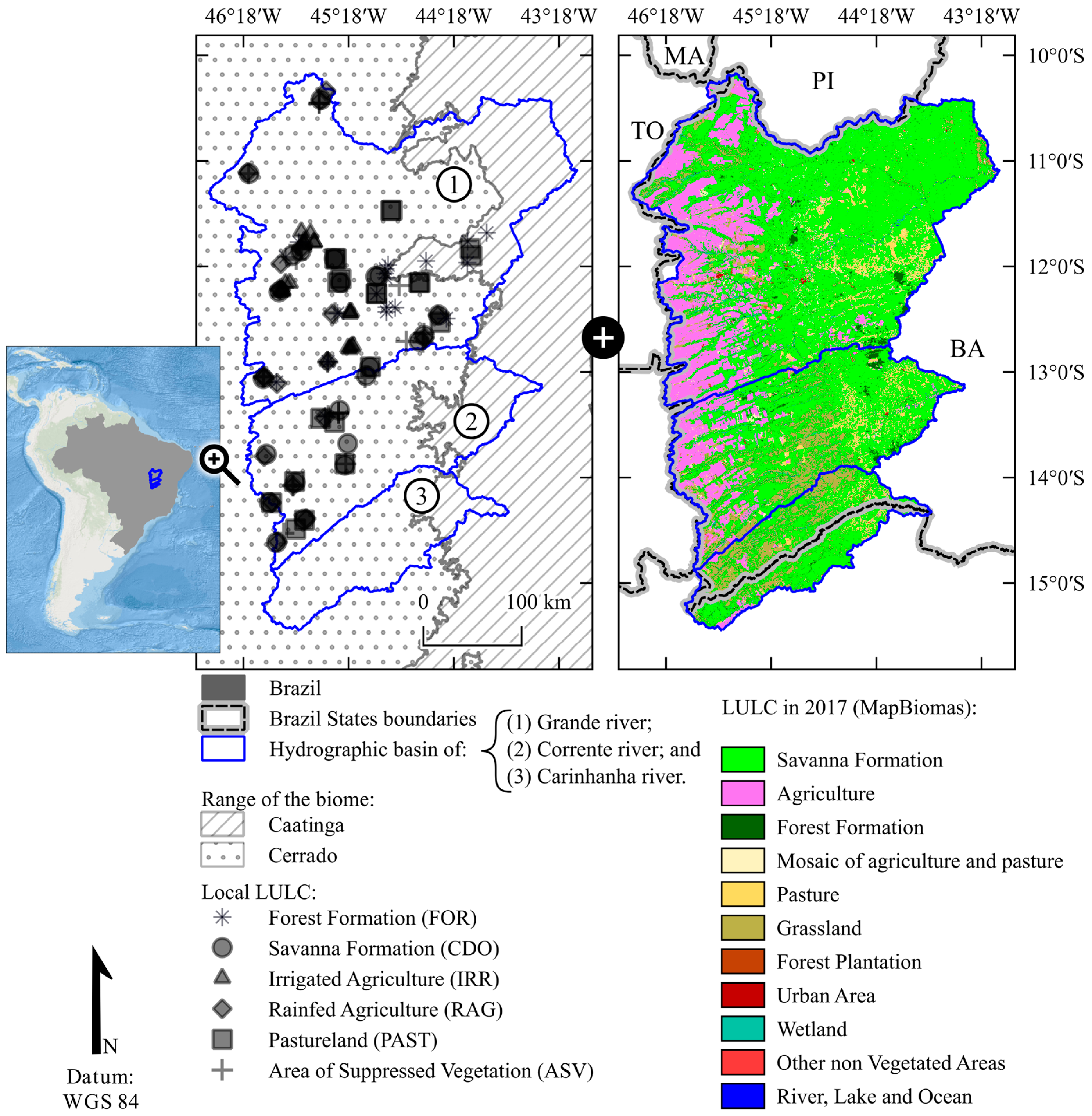
2.1. Study Area and Field Data Collection

The field soil data survey was conducted in the hydrographic basins of the rivers Grande, Corrente, and Carinhanha, in the western region of the state of Bahia, Brazil (Figure 1). The study area, located in the Cerrado biome, has a tropical climate with dry winter (climate Aw, in Köppen climate typology, Alvares et al. [26]) (Figure S1 of the Supplementary Material). The mean rainfall precipitation in the region (1980 to 2015) is 1060 mm year⁻¹, with great seasonality: There is low precipitation in the driest months (10 mm month⁻¹ in June, July, and August) and high precipitation in December and January (150 to 200 mm month⁻¹) [27]. The study area is located in a transition zone between the Cerrado biome (with annual precipitation greater than 1200 mm year⁻¹) and the Caatinga biome (with precipitation < 800 mm year⁻¹) [27].

The relief is predominantly flat (Figure S2). On the western edge of the basins, elevation reaches more than 1000 m above sea level, while at the mouth of the basin (easternmost region), the elevation is around 380 m. The landscape in the region, especially on the western border, is composed of formations known as Chapadões [28]. These relief characteristics favor agricultural mechanization and the use of chemical inputs in agriculture, so western Bahia is an important producing region of temporary crops (corn, soybeans, cotton, etc.) and constitutes the most recent Brazilian agricultural frontier, the MATOPIBA (acronym formed from the abbreviations of the states of Maranhão, Tocantins, Piauí, and Bahia) [27].

The soils of the region are formed on the geological formation of the Urucuia Group (dated to the Upper Cretaceous), whose composition includes quartz arenites, sandstones, and argillites [29]. The soils under study are predominantly sandy (with clay contents lower than 40% and total sand contents higher than 70%; see Figure 2b). According to the soil mapping of Brazil (Figure S3), following the criteria of the Brazilian Soil Classification System [30] and its correspondence with the World Reference Base for Soil Resources, there is a predominance in the region of Ferralsols, Arenosols, and Leptosols.

Soil-profile samples were collected from six different land-use and land-cover classes (LULC, observed on site), these being Cerrado (CDO: 23 sampled profiles), forest formation (FOR, 19 profiles), rainfed agriculture (RAG, 20 profiles), irrigated agriculture (IRR, 20 profiles), pastureland (PAST, 21 profiles), and area of suppressed vegetation (ASV, 20 profiles) [28], totaling 123 soil profiles. RAG and IRR areas are used to grow soybean (Glycine max), corn (Zea mays), cotton (Gossypium spp.), and beans (Phaseolus vulgaris). The CDO class is represented by Cerrado sensu stricto and grasslands, while the FOR class areas are represented by forest and Cerradão strata. The PAST class includes well-managed cultivated pastures and degraded pastures. Finally, the ASV class represents areas with recently suppressed vegetation. Images of the LULC classes of the sample points can be seen in [31].

In the IRR class, the samples were collected in the middle of the growing season in July 2017, while the RAG class samples were collected at the beginning of the growing season in November and December 2017. For the CDO, FOR, PAST, and ASV classes, the samples were also collected in November and December 2017.

Figure 1. Location of the sampled soil profiles in the study area and their respective LULC classes observed on site, accompanied by the LULC map of the basins (MapBiomas Collection 7.0 [32]). Hydrographic basins boundaries: Brazilian National Agency for Water and Basic Sanitation (ANA, https://dadosabertos.ana.gov.br/ (accessed on 24 April 2023)); geopolitical divisions: Brazilian Institute for Geography and Statistics (IBGE, https://portaldemapas.ibge.gov.br/ (accessed on 24 April 2023)).

Figure 1. Location of the sampled soil profiles in the study area and their respective LULC classes observed on site, accompanied by the LULC map of the basins (MapBiomas Collection 7.0 [32]). Hydrographic basins boundaries: Brazilian National Agency for Water and Basic Sanitation (ANA, https://dadosabertos.ana.gov.br/ (accessed on 24 April 2023)); geopolitical divisions: Brazilian Institute for Geography and Statistics (IBGE, https://portaldemapas.ibge.gov.br/ (accessed on 24 April 2023)).

Deformed soil samples were collected at seven depths in the 123 soil profiles: 0–5, 5–10, 10–15, 15–20, 20–40, 40–60, and 60–100 cm, totaling 861 samples. Each undeformed sample was composed of three subsamples, which were homogenized in the field. These samples were analyzed to quantify granulometry (fine sand, coarse sand, clay, and silt contents (kg kg⁻¹) of the superficial layer) and soil organic carbon (SOC (g kg⁻¹) of all 861 samples), whose analytical determination was carried out by the Walkley–Black colorimetric method [33]. The histogram of the SOC distribution and the texture distribution of the studied soils can be seen in Figure 2a and Figure 2b, respectively.

Figure 2. Histograms of soil organic carbon (SOC) contents in each soil layer (a) and soil texture diagram displaying the texture distribution of the surface layer (0–5 cm) of the sampled points (b).

Figure 2. Histograms of soil organic carbon (SOC) contents in each soil layer (a) and soil texture diagram displaying the texture distribution of the surface layer (0–5 cm) of the sampled points (b).

2.2. Remote Sensing Data Acquisition and Processing

The remote sensing data used in this study were derived from images from the SAR sensor onboard the orbital platform of the Sentinel-1A mission, the first satellite of the Sentinel-1 constellation of the European Space Agency (ESA). The Sentinel-1 mission satellites operate with SAR-type imaging radar sensors, a category of active sensors, and in the case of the Sentinel-1 satellites, the SAR sensors carry a C-band radar ($\lambda \cong 5.4 \mathrm{G}\mathrm{H}\mathrm{z}$) [34].

Dual-polarization images from the interferometric wide swath (IW) beam mode, which are images preprocessed with only the observed wave amplitude information, called GRD (ground range detected) products, were used. The Sentinel-1 bands with the greatest global coverage are the dual-polarization VH (where the sensor emits a pulse of radiation in vertical polarization and measures the detected reflectivity in horizontal polarization) and VV (emission and detection in vertical polarization). Sentinel-1 IW GRD images are formed after the sensor scans the Earth’s surface in three sub-swaths, i.e., IW1, IW2, and IW3, with ellipsoid incidence angles of 32.9, 28.3, and 43.1 and azimuthal resolutions (spatial resolution concerning the direction of flight of the satellite) of 22.4, 22.5, and 22.6 m, respectively [35].

The Sentinel-1 IW GRD images used in this work are detailed in

Table 1. Inventory of Sentinel-1 IW GRD images used in the study, generated by the SAR sensor of the Sentinel-1A satellite.

Acquisition Date	Product Unique Identifier	Relative Orbit Number
6 July 2017	B8D5	126
6 July 2017	0966
1 November 2017	82D6
1 November 2017	D608
1 November 2017	1ADD
1 November 2017	3E97
8 November 2017	3366	24

. and were obtained from the Alaska Satellite Facility (ASF) portal (https://asf.alaska.edu/, [36]). Although the products available on the ASF are not analysis-ready data like the Sentinel-1 imagery available via Google Earth Engine, the time series of radar imagery available on the ASF are readily available for download, which is no longer the case for the official ESA portal (the Copernicus Open-Access Hub) since the implementation of the long-term archive policy.

The processing steps (of the Table 1 products) and the algorithms used were as follows: (1) apply orbit file to obtain accurate satellite orbit and velocity vectors and generate accurate georeferencing of the images; (2) thermal noise removal to remove thermal antenna noise affecting the images; (3) border noise removal to remove noise on the edges of the images; (4) radiometric calibration to normalize the amplitude observed in each band for a radar cross-section and obtain the backscattering coefficient (reflectivity per unit area) in ${\beta }^0$ (section necessary to perform radiometric terrain corrections); (5) application of Speckle noise filter, in which the Lee filter was applied with a 5 × 5 pixels window; (6) the application of the radiometric terrain flattening algorithm attenuate geometrical distortions in the backscattering that are likely to occur due to the presence of relief artifacts (slopes, hills, etc.) and the operating geometry of SAR sensors (side-looking type) [37], and in this step, the backscattering coefficient is transformed from ${\beta }^0$ to ${\gamma }^0$; and (7) orthorectification of the images using the range-Doppler terrain correction algorithm. Details of the cited processing steps can be obtained in the texts by Filipponi [38] and dos Santos et al. [24].

Having the images with the VH and VV polarizations calibrated for the backscattering coefficient in ${\gamma }^0$, the next step was to compute the SAR vegetation indices. The SAR indices applied were as follows: RVIm (a proxy of the RVI for dual-polarized data) [39]; the normalized polarization index (Pol) [40], which calculates the normalized difference between VH and VV; the cross-ratio (CR), which is the ratio of VV by VH [41]; the dual-polarization SAR vegetation index (DPSVI) [23]; and the modified DPSVI (DPSVIm) index [24]. In addition to the aforementioned indices, the dual-polarization RVI for GRD products (DpRVIc) were also calculated [42]. The mathematical notation of each index used is presented in

Table 2. Description of synthetic aperture radar vegetation indices calculated with Sentinel-1 IW GRD images.

Vegetation Index	Equation	Theoretical Bounds	Source
DPSVI	$DPSV{I}_{(i,j)}=\frac{{VH}_{(i,j)}\left[\begin{array}{c}\left({VV}_{max}·{VH}_{(i,j)}-{VV}_{(i,j)}·{VH}_{(i,j)}+{{VH}_{(i,j)}}^2\right)+\\ \left({VV}_{max}·{VV}_{(i,j)}-{{VV}_{(i,j)}}^2+{VH}_{(i,j)}·{VV}_{(i,j)}\right)\end{array}\right]}{\sqrt{2}·{VV}_{(i,j)}}$	$0\le DPSVI$	[23]
DPSVIm	${DPSVIm}_{(i,j)}=\frac{{VV}_{(i,j)}^2+V{V}_{(i,j)}·V{H}_{(i,j)}}{\sqrt{2}}$	$0\le DPSVIm$	[24]
CR	${CR}_{(i,j)}=\frac{V{V}_{(i,j)}}{V{H}_{(i,j)}}$	$1\le CR$	[41]
Pol	${Pol}_{(i,j)}=\frac{V{H}_{(i,j)}-V{V}_{(i,j)}}{V{H}_{(i,j)}+V{V}_{(i,j)}}$	$-1\le Pol\le 1$	[40]
RVIm	${RVIm}_{(i,j)}=\frac{4V{H}_{(i,j)}}{V{H}_{(i,j)}+V{V}_{(i,j)}}$	Unreported	[39]
DpRVIc	${DpRVIc}_{(i,j)}=\frac{q_{(i,j)}·\left(q_{(i,j)}+3\right)}{{\left(1+q_{(i,j)}\right)}^2}$$; \mathrm{where} q_{(i,j)}=\frac{V{H}_{(i,j)}}{V{V}_{(i,j)}}$	$0\le DpRVIc\le 1$	[42]

Note: VV(i, j) and VH(i, j) correspond to the backscattering coefficient of the VV and VH polarizations at pixel (i, j).

.

The presented indices can be divided into cross-pol ratios (CR, RVIm, and Pol) and based on the degree of depolarization of the radar signal (DPSVI, DPSVIm, and DpRVIc). The Pol index is a normalized difference between the vertical dual polarization that was already employed to monitor crops in the study region by Filgueiras et al. [43], while the RVI is an adaptation of the original RVI index to be used with Sentinel-1 dual-polarization images. CR, on the other hand, is a ratio between the co-polarized image (VV) and the cross-polarized image (VH) and is commonly employed as an indicator of the presence of vegetation [13,41].

The DPSVI and DPSVIm indices use the concept of signal depolarization and quantify this depolarization using contrasts between the backscattering of the VH and VV polarizations and even separate bare soil and water surface (which always appear with values closer to zero) from vegetation pixels [23,24]. The DpRVIc index incorporates polarimetric descriptors and the degree of polarization (known as DoP; degree of polarization) measure from the original RVI to detect vegetation structure (branches, leaves, etc.) and has been tested to differentiate phenological stages of temporary crops [42].

The DPSVI, DPSVIm, and DpRVIc indices were calculated with the backscattering coefficient of the VV and VH polarizations in linear power units (dimensionless), while the CR, Pol, and RVIm indices were calculated with the backscattering coefficient transformed into the physical unit (decibel; dB), using Equation (1).

$${\gamma }^0\left(in dB\right)=10·{\log }_{10}{\gamma }^0$$

(1)

where ${\gamma }^0$ represents the backscattering coefficient of the VV and VH polarizations in unit linear power units, and ${\gamma }^0(in dB)$ is the same coefficient transformed to dB.

The download of the images, the processing, and the calculation of the vegetation indices was performed with Python programming language resources, using the SNAP (Sentinel Application Platform, version 9.0.6) software algorithms, and the raster sampling using the geographic coordinates of the soil profiles was performed with R programming language [44]. The codes built to process the Sentinel-1 IW GRD images from Table 1 can be found in the repository: <https://github.com/eupassarinho/sentinel-1-SAR-vegetation-indices.git>.

2.3. Modeling Soil Organic Carbon by Machine Learning Methods

In the processing of modeling SOC (g kg⁻¹), the vegetation indices of Table 2 plus the VV and VH polarizations (both in linear power unit as well as in dB) were used as predictors of SOC. To predict the SOC contents, three regression methods were employed: the least absolute shrinkage and selection operator (LASSO) [45], the support vector machine (SVM) [46] for regression (SVR), and the random forest (RF) [47]. These were chosen to encompass the modeling process methods based on linear (LASSO), nonlinear (SVR), and tree (RF) regression.

RF and SVM methods are already widely employed in soil attribute prediction and in digital soil mapping [17,48,49] and can be applied to both regression and classification problems. RF for regression works by building a collection of $M$ regression trees that are random to each other. Then, the average prediction of all trees is taken to predict a value [47,50]. On the other hand, the support vector machine admits predictions with a tolerable error, controlled by the modeling support vectors and defined by the hyperparameter C (cos) [51]. SVR becomes a nonlinear regression method when a nonlinear kernel function is used to transform the covariates as a preprocessing step for the prediction [51]. In this study, the kernel function used was the radial basis function (RBF).

Unlike RF and SVM, LASSO is a regression-only method, which selects predictors by penalty and also deals with the collinearity among them. LASSO fits linear regressions between the dependent variable and the predictors via ordinary least squares while adjusting the penalty parameter ($\lambda$) [52]. The hyperparameter $\lambda$ is used by the algorithm to force the parameter ${\beta }_1$ of each predictor to tend towards zero. If the ${\beta }_1$ of a predictor equals zero, then that predictor is not used in the prediction.

Regression methods are sensitive to the correlation that exists between the predictors [53,54]. This is the case for linear regression, SVM, and RF [17,48,49,55]. Therefore, before splitting the data for training the models, a correlation filter was applied with a threshold equal to 0.80. That is, of the covariables (Gamma0_VV, Gamma0_VH, Gamma0_VV_dB, Gamma0_VH_dB, Pol, RVIm, CR, DPSVI, DPSVIm, and DpRVIc), any with a correlation $\left|r\right|\ge 0.80$ [1,20] were eliminated from the modeling. This step, however, was employed only for modeling with the SVR-RBF and RF methods since LASSO deals with multicollinearity.

The original dataset (n = 861), containing SOC samples and the ten radar predictors, was randomly divided into the training and test (holdout) subsets, containing 70% and 30%, respectively, of the original data set [56]. However, since there is only one value of each covariate per soil profile, the models were trained for each soil layer [18,57], which means that each model was trained on 86 samples and tested on another 37 samples.

The models were then trained using k-fold cross-validation as the validation method for fitting the hyperparameters of the regression algorithms and 10 folds were defined [56]. For RF, the adjusted hyperparameter was the mtry (the number of predictor covariables to be used in each regression tree), which was set as 1/3 of the predictors (after filtering for correlation). For SVR-RBF, the C (cost) and sigma hyperparameters were tuned using a search grid ($C=\{0.1,0.2,0.4,0.6,0.8,1.0, and 10.0\}$, $sigma=\{0.0001,0.001,0.01,1/5(or 1/n of predictors),\mathrm{a}\mathrm{n}\mathrm{d} 1.0\}$). For the LASSO models, the hyperparameter $\lambda$ was tuned via search grid. The search grid for $\lambda$ was defined as an arithmetic progression of decimal numbers increasing from 0.0 to 2.0 every 0.2. For SVR-RBF and LASSO, preprocessing steps of the predictors were applied: centering (using the mean) and scaling (by the standard deviation).

For each regression method and soil layer, 100 models (or repetitions) were generated; for example, in the 0–5 cm layer, 100 models were generated with the SVR-RBF method and so on. This was carried out by setting, in each iteration of the loop, a new randomization seed coming from a truly random number. This methodology allows that in the sub-sampling process of the cross-validation, at each repetition, different data are in the k-folds and are used to adjust the hyperparameters of the model. Thus, it is possible to assess the degree of uncertainty of the models to the input data [48,54,57]. Since there are seven soil layers and three regression methods, this means that 2100 SOC prediction models were fitted. The modeling methodology is displayed in Figure 3.

All modeling steps were performed with R programming language resources, using functions from the tidymodels and caret (classification and regression training) packages, whose kernels for the regression methods were the glmnet (for LASSO), kernlab (for SVR-RBF), and randomForest (for RF) packages.

2.4. Results Assessment

The 2100 models were evaluated in both their training and prediction of samples from the test data set, and model performance analysis in both stages was performed to evaluate the generalization ability of the models. The evaluation of model performance in the training stage was carried out using the RMSE (root mean squared error) and R² (determination coefficient) metrics, which are standard caret accuracy and correlation metrics, respectively. To evaluate the predictions in the holdout test, other metrics were included: Willmott’s concordance index (d), MBE (mean bias error), MAE (mean absolute error), and CCC (Lin’s concordance correlation coefficient).

The 21 model architectures (e.g., RF for soil layer 0–5 cm, etc.) were compared to each other using non-parametric statistical tests. Since each model architecture generated 100 values for each statistical metric mentioned (MBE, RMSE, MAE, R², CCC, and d), the goal of this step was to test for statistically significant differences in the performance of models trained with different architectures (e.g., RMSE of RF versus RMSE of SVR-RBF for the 0–5 cm soil layer, etc.). For this, the Kruskal–Wallis’s test (non-parametric test for three or more groups of continuous variables) and Dunn’s test (post hoc pairwise test of the Kruskal–Wallis’s test) [58] were used, adopting a 95% confidence interval ($P=0.05$).

To assess the importance of the predictors in SOC modeling, the variable importance plots (VIP) method was used. The importance of the covariables used in the LASSO models consists of the normalization (from 0 to 100) of the slope coefficient (${\beta }_1$) adjusted for the covariables used by the method. For the SVM and RF methods, the importance is obtained by permuting a covariable in the model and evaluating the loss of model accuracy.

3. Results

3.1. Accuracy of Soil Organic Carbon Prediction

For predicting soil organic carbon (SOC) contents, not all covariables obtained from the processing of Sentinel-1 images were used. The linear correlation diagram between the covariables was obtained (Figure 4), where we noticed that although each covariable comes from a different equation, some are highly correlated. This is the case for the covariables CR, Pol, and RVIm, which are ratios between the radar polarizations, in addition to the VV and VH polarizations (both in linear power units and in dB). Therefore, after filtering covariables for multicollinearity ($r\ge 0.80)$ to feed the SVR-RBF and RF regression methods, the predictors DPSVIm, DPSVI, Gamma0_VH, DpRVIc, and CR were selected. For the LASSO method, all covariables in Figure 4 were employed.

Having filtered out the covariables to be used in modeling, the prediction of SOC by the different regression methods was evaluated in two steps: the performance of the models in the cross-validation step and in the holdout test (with samples not used to train the models).

Figure 5 exhibits the results of the goodness-of-fit metrics (RMSE and R²) obtained in the cross-validation of each model in each soil layer; in other words, the optimization results of the hyperparameters of each model are reported. In general, for both RMSE and R², there are significant differences between the fitting of each soil layer and each regression method, according to the non-parametric Kruskal–Wallis test. In addition, Dunn’s pairwise test indicates that the models of the deeper layers (>20 to 100 cm) and the topsoil layers (0 to 20 cm depth) are more similar to each other. Detailed results of the statistical tests can be found in the Supplementary Material.

We observe that the RMSE obtained in the SOC modeling is of the order of 5.5 g kg⁻¹ in the topsoil layers and decreases as the soil depth increases. With R², median values of around 0.2 were obtained in the topsoil layers, tending to decrease in deeper layers.

The RMSE of the deeper soil layers, of the order of 2.0 to 3.5 g kg⁻¹, suggests that as the depth increases, the models become more accurate. However, this is mainly due to the smaller amplitude of the data in these layers, as we observe the distribution of SOC (g kg⁻¹) for the layers 20–40, 40–60, and 60–100 cm in Figure 2. In addition, the median R² of the deeper layers, close to 0.1 for the LASSO and RF methods, indicates that the set of predictors explains less SOC variation than in the topsoil layers.

The loss of correlation between SOC estimates and observations as soil depth increases could also be evidenced in the test results obtained from new soil samples.

Table 3. Model performance results in the holdout test: median (Md) of MBE (mean bias error), RMSE (root mean squared error), MAE (mean absolute error), R² (coefficient of determination), CCC (Lin’s concordance correlation coefficient), and d (Willmott’s concordance index).

Regression Method	Soil Layer	Md (MBE)	Md (RMSE)	Md (MAE)	Md (R2)	Md (CCC)	Md (d)
LASSO	0–5 cm	0.869	4.864	3.914	0.243	0.231	0.442
	5–10 cm	−1.248	5.135	3.869	0.167	0.127	0.345
	10–15 cm	−0.824	5.557	4.532	0.027	0.079	0.297
	15–20 cm	−0.727	4.099	3.489	0.059	0.083	0.291
	20–40 cm	0.670	3.912	3.278	0.007	0.050	0.314
	40–60 cm	−0.005	2.414	1.956	0.001	0.017	0.318
	60–100 cm	0.093	2.322	2.015	0.000	−0.004	0.167
SVR-RBF	0–5 cm	0.899	4.959	3.942	0.238	0.196	0.400
	5–10 cm	−0.989	4.953	3.686	0.172	0.212	0.452
	10–15 cm	−1.123	5.556	4.582	0.039	0.086	0.325
	15–20 cm	−0.812	4.213	3.513	0.015	0.053	0.362
	20–40 cm	0.824	3.876	3.307	0.002	0.021	0.265
	40–60 cm	−0.035	2.306	1.928	0.040	0.042	0.193
	60–100 cm	0.285	2.436	2.151	0.011	−0.043	0.135
RF	0–5 cm	0.777	4.955	3.898	0.208	0.184	0.360
	5–10 cm	−1.196	5.082	3.829	0.180	0.151	0.372
	10–15 cm	−1.084	5.670	4.724	0.003	0.016	0.236
	15–20 cm	−0.666	4.187	3.567	0.015	0.046	0.294
	20–40 cm	0.740	3.811	3.219	0.010	0.037	0.272
	40–60 cm	−0.064	2.304	1.899	0.034	0.067	0.287
	60–100 cm	0.110	2.297	2.014	0.003	0.007	0.129

is a summary of the models’ performance in the holdout test, and it shows the median value (Md) of the statistical metrics: MBE, RMSE, MAE, R², CCC, and d. From Table 3, we notice that the best correlation (R²) and agreement (CCC and d) values were obtained with the models for the 0–5 cm and 5–10 cm (topsoil) layers.

Among the metrics R², CCC, and d, the d index shows the highest values of agreement between SOC estimates and observations (Table 3). However, the results obtained with R² and CCC metrics indicate that around 20% of the SOC variability was explained with the radar covariables, mainly in the topsoil layers: 0–5 cm and 5–10 cm. For these layers, whose results are highlighted in Table 3, the best results were obtained with the SVR-RBF and LASSO regression methods, which showed better generalization ability than the models trained with RF.

3.2. Covariables’ Importance and Their Relationship to Soil Organic Carbon

As demonstrated by the analysis of Figure 5 and Table 3, the predictive ability of the radar covariates was better for the topsoil layers (0–5 cm and 5–10 cm). Considering the similarity of accuracy and correlation for both layers, the analysis of the importance of the covariates is presented only for the 0–5 cm layer and for each model architecture (Figure 6).

Figure 6 displays boxplots with the importance of each covariable used in the SOC modeling. In the graph in Figure 6a, each covariable has many importance values according to the number of times it was used by the LASSO method. On the other hand, in Figure 6b,c, each covariable has 100 importance values from the 100 SVR-RBF and RF models, respectively.

For the linear method, LASSO, the most important covariable, the VH polarization of the Sentinel-1 sensor was present in almost all models. In turn, the VV polarization (in dB) was also selected for most models but with less importance and more similar to the DPSVIm index. Other covariables were used in some models: the VV polarization in linear power units, the DPSVI index, and the CR ratio.

The VH polarization was also the most important covariable for the SVR-RBF and RF models. In the case of these models, the method of estimating importance is based on the loss of prediction accuracy when a particular covariable is removed from the model. This means that although the VH band is the covariable that most contributes to the prediction accuracy, the vegetation indices also contributed to the SOC estimates.

For the 0–5 cm layer, it is possible to differentiate the distribution of SOC content between each land-use and land-cover class (LULC) where the samples were collected. In Figure 7, we observe that the SOC values tend to increase from the pasture class (PAST) towards the forest formations (FLO). The lowest SOC contents are observed in the PAST and rainfed agriculture (RAG) classes, intermediate SOC values are seen in the Cerrado savanna formation (CDO) and recently suppressed area (ASV) classes, while the highest SOC contents are in the irrigated agriculture (IRR) and forestry (FLO) classes.

The same behavior was observed in SOC contents among LULC classes, with contents increasing from the PAST class to FLO class, as we observed in other covariables. The covariables DPSVI, DPSVIm, Gamma0_VH, and Gamma0_VV_dB also showed similar behavior to the SOC contents, and in the case of the DPSVIm index, we observed that it tends to separate the FLO (with the highest SOC contents) class from the others. The CR index has an inversely proportional behavior: The values tend to decrease from the PAST to the FLO classes, although the only class that differed from the others was the PAST class. Also, in the case of DpRVIc, there was no behavior similar to SOC among the LULC classes.

4. Discussion

Zhou, Geng, Chen, Pan, et al. [20] performed SOC prediction (with contents ranging from 4.70 to 439.10 g kg⁻¹) in a central European region (in the countries of Slovenia, Austria, and Italy), in which one of the experiments consisted of predicting SOC contents using as predictors only the VV and VH polarizations of Sentinel-1 IW GRD images. The modeling developed by the authors used soil samples from the 0 to 20 cm layer. Although the dimensional accuracy metrics (RMSE and MAE) employed by the authors cannot be compared since they applied transformations to the modeled SOC samples, for both regression methods (SVM and RF), the authors obtained an R² of 0.16.

In similar modeling work, Zhou, Geng, Chen, Liu, et al. [19] obtained a goodness-of-fit $R^2=0.19$ in SOC predicting. In this work, the authors also used Sentinel-1 IW GRD imagery (also only the backscattering coefficients) and the RF regression method to predict SOC (with contents ranging from 1.75 to 139.83 g kg⁻¹) in a hydrographic basin in China in high-altitude and low-temperature terrain. In the present work, we achieved R² values between predictions and observations of SOC contents (with contents ranging from 0.59 to 26.91 g kg⁻¹) in testing the models of the order of $R^2~0.24$ using the LASSO and SVR-RBF algorithms in models of the topsoil layers (see Figure 5 and Table 3).

In addition, the models achieved RMSE values between 4 and 6 g kg⁻¹ (Table 3). These accuracy values found are comparable to regression models that use the spectral signature of soil samples to predict SOC. In these types of studies, authors found RMSE values ranging from 1.0 to 7.0 g kg⁻¹, as can be seen in the work of Soriano-Disla et al. [59] and Santos et al. [60], even though the values of R² in studies at the spectroscopic scale are of the order of two to three times higher than the values of R² found in our study with SAR remote sensing. Similarly, Moura-Bueno et al. [61] found RMSE values between 4.0 and 12 g kg⁻¹ in the prediction of SOC in southern Brazil by the utilizing spectral signatures (in the visible and near-infrared spectral regions) of soil samples. According to the authors, these variations in accuracy were related to pedological and environmental characteristics, including soil texture and type of land use and land cover.

The best-performing regression methods were the linear method, LASSO, and nonlinear SVR-RBF, to the detriment of RF (see Table 3), a behavior also observed by Shafizadeh-Moghadam et al. [17]. This suggests that there is a linear (or quasi-linear) relationship between the covariables and SOC contents. In this sense, it is important to highlight how the radar covariables and SOC contents behave in the different LULC classes in which the soil samples were collected, as the influence that the type of LULC has on SOC variations, especially in the topsoil layers, is well known [62].

At landscape scales (and larger scales), vegetation type and LULC class are factors that control SOC (along with other factors), and this is due to the control that organisms exert over the rates of organic matter input and decomposition [62,63]. In the topsoil layer, we noticed that SOC contents vary according to the type of vegetation (Figure 7). In Figure 6, we note the relative importance that the variables DPSVI, DPSVIm, and the VH polarization have for predicting SOC contents, and in Figure 7, we note that these same radar covariates showed similar behavior to the SOC contents in each LULC class. The ability of the Sentinel-1 covariables to stratify the different vegetation types indicates why the topsoil layer models were able to explain around 20% of the variation in SOC contents in the studied soils in contrast to the models from deeper layers (Table 3).

The capability of Sentinel-1 covariates to account for approximately 20% of the variability in soil organic carbon (SOC) contents across landscapes may be perceived as limited. However, it is important to consider that, for the purposes of digital soil mapping, additional covariates representing soil-forming factors are required to achieve more accurate predictions [10]. Take, for example, the SCORPAN framework, in which various elements such as the soil properties itself, climate, living organisms, relief descriptors, parent material, age, and geographical location are integrated to model complex phenomena contributing to spatial variations in soil properties [10].

Nonetheless, studies that focus on isolated groups of predictors (e.g., those representing only organisms in a specific location, as in the present study) tend to yield low R² values [4,17,19,20]. It is important to note, however, that a low R² value does not necessarily indicate a lack of predictive ability. The concept of “low” accuracy in digital soil mapping is relative given that the pedosphere is an intricate Earth system with landscape variations that are challenging to capture, even when considering all the covariates within the SCORPAN framework.

The covariables obtained from the SAR images contributed differently to the SOC prediction modeling (Figure 6). The VH polarization was the most-used covariable for the LASSO method and the one with the greatest relative importance for the SVR-RBF and RF methods. Although the intensity of the backscattered radar signal for SAR sensors is not a direct measure of aboveground plant biomass [64], the backscatter observed in HV or VH cross-polarization bands is directly associated with aboveground biomass [12,65,66,67]. This is because for cross-polarization bands, only surface elements that change the polarization of the electromagnetic wave reflected to the sensor are detected with higher brightness, and this is the case for vegetation [68]. Vegetation is a type of target in which microwaves, with wavelengths ranging from ~2 cm to 1 m, interact and undergo a change in their polarization, a mechanism known as volumetric backscattering [13].

The contribution of the SAR vegetation indices to the SOC prediction models is due to the purpose of each of the indices when they were proposed. DpRVI is an adaptation for GRD products of the DpRVI index of Mandal et al. [25], which in turn is an RVI-based index whose formulation is conceptually based on the degree of polarization of microwaves as they interact with vegetation [25,42]. The degree of polarization measures how much of the total energy backscattered by the targets has had its polarization changed. Both DpRVI and DpRVIc have been successful in discretizing phenological stages in annual crops such as canola, wheat, corn, etc.

DPSVI is also based on the depolarization of the microwave signal, but its structure also seeks to distinguish areas of water bodies and bare-ground surfaces. To this end, the DPSVI takes in its formulation the Euclidean distance relationships between the VV and VH backscattering to distinguish these conditions, also incorporating the VH polarization to graduate different levels of biomass in vegetation [23], and was originally tested on crops such as cassava and corn. Taking advantage of the concept of signal degree of depolarization, dos Santos et al. [24] proposed modifications in the DPSVI model to make the index more sensitive to different levels of biomass in forest-like areas. Among the modifications made, dos Santos et al. [24] incorporated the CR index, which facilitates the separation of different biomass levels in forest areas.

Since the soil samples used were collected in different LULC situations, from pastures to forested areas in the Brazilian Cerrado, and considering the applicability of the different SAR indices, we can affirm that there is a contribution of the different indices for SOC prediction in all regression methods in the topsoil layers. In addition to this, the prediction of SOC using Sentinel-1 IW GRD imagery products is feasible due to the ability to monitor the surface plant biomass and not the soil itself because, as shown by El Hajj et al. [69] and Saatchi [12], there is low C-band microwave penetration in vegetated areas.

SOC modeling in the landscape has historically had the contribution of optical vegetation indices to directly represent land cover and indirectly represent the condition of use and cover by the stratum of that vegetation in addition to other remote sensing products (such as net primary productivity) that denote the input of organic carbon to the soil from plant organs [4,18,57]. Optical vegetation indices represent the biophysical, biochemical, and physiological properties of the mapped vegetation, as shown in the systematic review by de Zeng et al. [70]. On the other hand, SAR vegetation indices tend to represent the vegetation structure, i.e., its geometry according to the vegetation type. Therefore, they can contribute to digital soil-mapping studies—even taking advantage of the continuity of operational space missions such as Sentinel-1—of missions that have recently become operational, such as the SAOCOM (Satélite Argentino de Observación Con Microondas) satellite constellation, which has L-band SAR sensors in the twin satellites (SAOCOM 1A and 1B), as well as planned missions such as NISAR (NASA-ISRO SAR), with L- and S-band sensors.

Furthermore, more accurate predictions of SOC content can be obtained by combining SAR-derived variables with covariables related to other SCORPAN components. In this regard, other components of SCORPAN, more precisely the relief, have already been described in studies of SOC modeling using SAR sensor images [71].

The use of SAR remote sensing data has already been proven to be an important alternative to optical remote sensing and has one major advantage over optical remote sensing. Imaging with SAR sensors is much less influenced by atmospheric conditions such as the presence of clouds [43,72] since microwaves (with $\lambda >2 \mathrm{c}\mathrm{m})$ barely interact with atmospheric particles [13,73]. This advantage ensures operationality when employing SAR imagery in digital soil-mapping works.

5. Conclusions

It was possible to predict the soil organic carbon (SOC) content of a region with different land-use and land-cover classes and predominantly sandy soils, using as explanatory variables the SAR (synthetic aperture radar) vegetation indices for Sentinel-1 satellite dual-polarization images.

The models fed with SAR sensor polarizations and their vegetation indices produced more accurate results in the topsoil layers (0–5 cm and 5–10 cm). In these superficial layers, the LASSO (least absolute shrinkage and selection operator), SVM (support vector machine), and RF (random forest) methods generated models with statistical metrics: RMSE of the order of 5.0 g kg⁻¹; MAE of the order of 3.9 g kg⁻¹; R² ranging from 0.16 to 0.24; CCC ranging from 0.12 to 0.23; and the d index ranging from 0.34 to 0.45. In deeper soil layers, although more accurate (looking at RMSE and MAE), the covariables lost their ability to explain SOC variability.

References

1. Lombardo, L.; Saia, S.; Schillaci, C.; Mai, P.M.; Huser, R. Modeling Soil Organic Carbon with Quantile Regression: Dissecting Predictors’ Effects on Carbon Stocks. Geoderma 2018, 318, 148–159. [Google Scholar] [CrossRef]
2. Yost, J.L.; Hartemink, A.E. Soil Organic Carbon in Sandy Soils: A Review. In Advances in Agronomy; Academic Press Inc.: London, UK, 2019; Volume 158, pp. 217–310. ISBN 978-0-12-817412-8. [Google Scholar]
3. FAO; ITPS. Global Soil Organic Carbon Map (GSOCmap) Version 1.5; FAO: Rome, Italy, 2020; ISBN 978-92-5-132144-7. [Google Scholar]
4. Kunkel, V.R.; Wells, T.; Hancock, G.R. Modelling Soil Organic Carbon Using Vegetation Indices across Large Catchments in Eastern Australia. Sci. Total Environ. 2022, 817, 152690. [Google Scholar] [CrossRef] [PubMed]
5. Padarian, J.; Minasny, B.; McBratney, A.; Smith, P. Soil Carbon Sequestration Potential in Global Croplands. PeerJ 2022, 10, e13740. [Google Scholar] [CrossRef]
6. Poggio, L.; de Sousa, L.M.; Batjes, N.H.; Heuvelink, G.B.M.; Kempen, B.; Ribeiro, E.; Rossiter, D. SoilGrids 2.0: Producing Soil Information for the Globe with Quantified Spatial Uncertainty. Soil 2021, 7, 217–240. [Google Scholar] [CrossRef]
7. Guo, L.; Zhang, H.; Shi, T.; Chen, Y.; Jiang, Q.; Linderman, M. Prediction of Soil Organic Carbon Stock by Laboratory Spectral Data and Airborne Hyperspectral Images. Geoderma 2019, 337, 32–41. [Google Scholar] [CrossRef]
8. Keskin, H.; Grunwald, S.; Harris, W.G. Digital Mapping of Soil Carbon Fractions with Machine Learning. Geoderma 2019, 339, 40–58. [Google Scholar] [CrossRef]
9. Odebiri, O.; Mutanga, O.; Odindi, J.; Peerbhay, K.; Dovey, S. Predicting Soil Organic Carbon Stocks under Commercial Forest Plantations in KwaZulu-Natal Province, South Africa Using Remotely Sensed Data. GIScience Remote Sens. 2020, 57, 450–463. [Google Scholar] [CrossRef]
10. McBratney, A.B.; Mendonça Santos, M.L.; Minasny, B. On Digital Soil Mapping. Geoderma 2003, 117, 3–52. [Google Scholar] [CrossRef]
11. Hole, F.D. Effects of Animals on Soil. Geoderma 1981, 25, 75–112. [Google Scholar] [CrossRef]
12. Saatchi, S. SAR Methods for Mapping and Monitoring Forest Biomass. In The Synthetic Aperture Radar (SAR) Handbook: Comprehensive Methodologies for Forest Monitoring and Biomass Estimation; Flores-Anderson, A.I., Herndon, K.E., Thapa, R.B., Cherrington, E., Eds.; NASA: Huntsville, AL, USA, 2019. [Google Scholar]
13. Woodhouse, I.H. Introduction to Microwave Remote Sensing; CRC Press: Boca Raton, FL, USA, 2006; ISBN 0-415-27123-1. [Google Scholar]
14. Paradella, W.R.; Mura, J.C.; Gama, F.F. Monitoramento DInSAR Para Mineração e Geotecnia; Oficina de Textos: São Paulo, Brazil, 2021; ISBN 978-65-86235-19-7. [Google Scholar]
15. Bartsch, A.; Widhalm, B.; Kuhry, P.; Hugelius, G.; Palmtag, J.; Siewert, M.B. Can C-Band Synthetic Aperture Radar Be Used to Estimate Soil Organic Carbon Storage in Tundra? Biogeosciences 2016, 13, 5453–5470. [Google Scholar] [CrossRef]
16. Ceddia, M.B.; Gomes, A.S.; Vasques, G.M.; Pinheiro, É.F.M. Soil Carbon Stock and Particle Size Fractions in the Central Amazon Predicted from Remotely Sensed Relief, Multispectral and Radar Data. Remote Sens. 2017, 9, 124. [Google Scholar] [CrossRef]
17. Shafizadeh-Moghadam, H.; Minaei, F.; Talebi-khiyavi, H.; Xu, T.; Homaee, M. Synergetic Use of Multi-Temporal Sentinel-1, Sentinel-2, NDVI, and Topographic Factors for Estimating Soil Organic Carbon. Catena 2022, 212, 106077. [Google Scholar] [CrossRef]
18. Sothe, C.; Gonsamo, A.; Arabian, J.; Snider, J. Large Scale Mapping of Soil Organic Carbon Concentration with 3D Machine Learning and Satellite Observations. Geoderma 2022, 405, 115402. [Google Scholar] [CrossRef]
19. Zhou, T.; Geng, Y.; Chen, J.; Liu, M.; Haase, D.; Lausch, A. Mapping Soil Organic Carbon Content Using Multi-Source Remote Sensing Variables in the Heihe River Basin in China. Ecol. Indic. 2020, 114, 106288. [Google Scholar] [CrossRef]
20. Zhou, T.; Geng, Y.; Chen, J.; Pan, J.; Haase, D.; Lausch, A. High-Resolution Digital Mapping of Soil Organic Carbon and Soil Total Nitrogen Using DEM Derivatives, Sentinel-1 and Sentinel-2 Data Based on Machine Learning Algorithms. Sci. Total Environ. 2020, 729, 138244. [Google Scholar] [CrossRef]
21. Kim, Y.; van Zyl, J. On the Relationship between Polarimetric Parameters. In Proceedings of the IGARSS 2000. IEEE 2000 International Geoscience and Remote Sensing Symposium. Taking the Pulse of the Planet: The Role of Remote Sensing in Managing the Environment. Proceedings (Cat. No.00CH37120), Honolulu, HI, USA, 24–28 July 2000; IEEE: New York, NY, USA, 2000; Volume 3, pp. 1298–1300. [Google Scholar]
22. Chang, J.G.; Shoshany, M.; Oh, Y. Polarimetric Radar Vegetation Index for Biomass Estimation in Desert Fringe Ecosystems. IEEE Trans. Geosci. Remote Sens. 2018, 56, 7102–7108. [Google Scholar] [CrossRef]
23. Periasamy, S. Significance of Dual Polarimetric Synthetic Aperture Radar in Biomass Retrieval: An Attempt on Sentinel-1. Remote Sens. Environ. 2018, 217, 537–549. [Google Scholar] [CrossRef]
24. dos Santos, E.P.; da Silva, D.D.; do Amaral, C.H. Vegetation Cover Monitoring in Tropical Regions Using SAR-C Dual-Polarization Index: Seasonal and Spatial Influences. Int. J. Remote Sens. 2021, 42, 7581–7609. [Google Scholar] [CrossRef]
25. Mandal, D.; Kumar, V.; Ratha, D.; Dey, S.; Bhattacharya, A.; Lopez-Sanchez, J.M.; McNairn, H.; Rao, Y.S. Dual Polarimetric Radar Vegetation Index for Crop Growth Monitoring Using Sentinel-1 SAR Data. Remote Sens. Environ. 2020, 247, 111954. [Google Scholar] [CrossRef]
26. Alvares, C.A.; Stape, J.L.; Sentelhas, P.C.; de Moraes Gonçalves, J.L.; Sparovek, G. Köppen’s Climate Classification Map for Brazil. Meteorol. Z. 2013, 22, 711–728. [Google Scholar] [CrossRef]
27. Pousa, R.; Costa, M.H.; Pimenta, F.M.; Fontes, V.C.; Castro, M. Climate Change and Intense Irrigation Growth in Western Bahia, Brazil: The Urgent Need for Hydroclimatic Monitoring. Water 2019, 11, 933. [Google Scholar] [CrossRef]
28. Dionizio, E.A.; Pimenta, F.M.; Lima, L.B.; Costa, M.H. Carbon Stocks and Dynamics of Different Land Uses on the Cerrado Agricultural Frontier. PLoS ONE 2020, 15, e0241637. [Google Scholar] [CrossRef] [PubMed]
29. SGB. GeoSGB; Serviço Geológico do Brasil: Brasília, Brazil, 2022.
30. dos Santos, H.G.; Jacomine, P.K.T.; dos Anjos, L.H.C.; de Oliveira, V.Á.; Lumbreras, J.F.; Coelho, M.R.; de Almeida, J.A.; de Araújo-Filho, J.C.; Cunha, T.J.F. Brazilian Soil Classification System, 5th ed.; Embrapa: Brasília, Brazil, 2018; ISBN 978-85-7035-800-4. [Google Scholar]
31. Dionizio, E.A.; Costa, M.H. Influence of Land Use and Land Cover on Hydraulic and Physical Soil Properties at the Cerrado Agricultural Frontier. Agriculture 2019, 9, 24. [Google Scholar] [CrossRef]
32. Souza, C.M.; Shimbo, J.Z.; Rosa, M.R.; Parente, L.L.; Alencar, A.A.; Rudorff, B.F.T.; Hasenack, H.; Matsumoto, M.; Ferreira, L.G.; Souza-Filho, P.W.M.; et al. Reconstructing Three Decades of Land Use and Land Cover Changes in Brazilian Biomes with Landsat Archive and Earth Engine. Remote Sens. 2020, 12, 2735. [Google Scholar] [CrossRef]
33. Walkley, A.; Black, I.A. An Examination of the Degtjareff Method for Determining Soil Organic Matter, and a Proposed Modification of the Chromic Acid Titration Method. Soil Sci. 1934, 37, 29–38. [Google Scholar] [CrossRef]
34. ESA. Sentinel-1: ESA’s Radar Observatory Mission for GMES Operational Services; Fletcher, K., Ed.; European Space Agency: Paris, France, 2012. [Google Scholar]
35. ESA. Sentinel-1 SAR Technical Guide. Available online: https://sentinel.esa.int/web/sentinel/technical-guides/sentinel-1-sar (accessed on 18 November 2022).
36. ASF Copernicus Sentinel Data 2017, 2018, and 2019. Retrieved from ASF DAAC, Processed by ESA. Available online: https://asf.alaska.edu/ (accessed on 17 November 2022).
37. Small, D. Flattening Gamma: Radiometric Terrain Correction for SAR Imagery. IEEE Trans. Geosci. Remote Sens. 2011, 49, 3081–3093. [Google Scholar] [CrossRef]
38. Filipponi, F. Supplementary Materials: Sentinel-1 GRD Preprocessing Workflow. Proceedings 2019, 18, 11. [Google Scholar] [CrossRef]
39. Nasirzadehdizaji, R.; Balik Sanli, F.; Abdikan, S.; Cakir, Z.; Sekertekin, A.; Ustuner, M. Sensitivity Analysis of Multi-Temporal Sentinel-1 SAR Parameters to Crop Height and Canopy Coverage. Appl. Sci. 2019, 9, 655. [Google Scholar] [CrossRef]
40. Hird, J.; DeLancey, E.; McDermid, G.; Kariyeva, J. Google Earth Engine, Open-Access Satellite Data, and Machine Learning in Support of Large-Area Probabilistic Wetland Mapping. Remote Sens. 2017, 9, 1315. [Google Scholar] [CrossRef]
41. Frison, P.-L.; Fruneau, B.; Kmiha, S.; Soudani, K.; Dufrêne, E.; Toan, T.L.; Koleck, T.; Villard, L.; Mougin, E.; Rudant, J.-P. Potential of Sentinel-1 Data for Monitoring Temperate Mixed Forest Phenology. Remote Sens. 2018, 10, 2049. [Google Scholar] [CrossRef]
42. Bhogapurapu, N.; Dey, S.; Mandal, D.; Bhattacharya, A.; Karthikeyan, L.; McNairn, H.; Rao, Y.S. Soil Moisture Retrieval over Croplands Using Dual-Pol L-Band GRD SAR Data. Remote Sens. Environ. 2022, 271, 112900. [Google Scholar] [CrossRef]
43. Filgueiras, R.; Mantovani, E.C.; Althoff, D.; Fernandes Filho, E.I.; Cunha, F.F. da Crop NDVI Monitoring Based on Sentinel 1. Remote Sens. 2019, 11, 1441. [Google Scholar] [CrossRef]
44. R Core Team. R: A Language and Environment for Statistical Computing; R Core Team: Vienna, Austria, 2023. [Google Scholar]
45. Tibshirani, R. Regression Shrinkage and Selection Via the Lasso. J. R. Stat. Soc. Ser. B Methodol. 1996, 58, 267–288. [Google Scholar] [CrossRef]
46. Cortes, C.; Vapnik, V. Support-Vector Networks. Mach. Learn. 1995, 20, 273–297. [Google Scholar] [CrossRef]
47. Breiman, L. Random Forests. Mach. Learn. 2001, 45, 5–32. [Google Scholar] [CrossRef]
48. Mishra, U.; Yeo, K.; Adhikari, K.; Riley, W.J.; Hoffman, F.M.; Hudson, C.; Gautam, S. Empirical Relationships between Environmental Factors and Soil Organic Carbon Produce Comparable Prediction Accuracy to Machine Learning. Soil Sci. Soc. Am. J. 2022, 86, 1611–1624. [Google Scholar] [CrossRef]
49. Xiao, Y.; Xue, J.; Zhang, X.; Wang, N.; Hong, Y.; Jiang, Y.; Zhou, Y.; Teng, H.; Hu, B.; Lugato, E.; et al. Improving Pedotransfer Functions for Predicting Soil Mineral Associated Organic Carbon by Ensemble Machine Learning. Geoderma 2022, 428, 116208. [Google Scholar] [CrossRef]
50. Biau, G.; Scornet, E. A Random Forest Guided Tour. Test 2016, 25, 197–227. [Google Scholar] [CrossRef]
51. Smola, A.J.; Schölkopf, B. A Tutorial on Support Vector Regression. Stat. Comput. 2004, 14, 199–222. [Google Scholar] [CrossRef]
52. James, G.; Witten, D.; Hastie, T.; Tibshirani, R. An Introduction to Statistical Learning; Springer Texts in Statistics; Springer: New York, NY, USA, 2013; Volume 103, ISBN 978-1-4614-7137-0. [Google Scholar]
53. Boehmke, B.; Greenwell, B. Hands-On Machine Learning with R; Chapman and Hall/CRC: Boca Raton, FL, USA, 2019; ISBN 978-0-367-81637-7. [Google Scholar]
54. Kuhn, M.; Johnson, K. Applied Predictive Modeling; Springer: New York, NY, USA, 2013; ISBN 978-1-4614-6848-6. [Google Scholar]
55. Moura-Bueno, J.M.; Dalmolin, R.S.D.; ten Caten, A.; Dotto, A.C.; Demattê, J.A.M. Stratification of a Local VIS-NIR-SWIR Spectral Library by Homogeneity Criteria Yields More Accurate Soil Organic Carbon Predictions. Geoderma 2019, 337, 565–581. [Google Scholar] [CrossRef]
56. Brus, D.J.; Kempen, B.; Heuvelink, G.B.M. Sampling for Validation of Digital Soil Maps. Eur. J. Soil Sci. 2011, 62, 394–407. [Google Scholar] [CrossRef]
57. Gomes, L.C.; Faria, R.M.; de Souza, E.; Veloso, G.V.; Schaefer, C.E.G.R.; Filho, E.I.F. Modelling and Mapping Soil Organic Carbon Stocks in Brazil. Geoderma 2019, 340, 337–350. [Google Scholar] [CrossRef]
58. McKight, P.E.; Najab, J. Kruskal-Wallis Test. In The Corsini Encyclopedia of Psychology; John Wiley & Sons, Ltd.: Hoboken, NJ, USA, 2010; p. 1. ISBN 978-0-470-47921-6. [Google Scholar]
59. Soriano-Disla, J.M.; Janik, L.J.; Viscarra Rossel, R.A.; Macdonald, L.M.; McLaughlin, M.J. The Performance of Visible, Near-, and Mid-Infrared Reflectance Spectroscopy for Prediction of Soil Physical, Chemical, and Biological Properties. Appl. Spectrosc. Rev. 2014, 49, 139–186. [Google Scholar] [CrossRef]
60. dos Santos, U.J.; de Demattê, J.A.M.; Menezes, R.S.C.; Dotto, A.C.; Guimarães, C.C.B.; Alves, B.J.R.; Primo, D.C.; Sampaio, E.V.d.S.B. Predicting Carbon and Nitrogen by Visible Near-Infrared (Vis-NIR) and Mid-Infrared (MIR) Spectroscopy in Soils of Northeast Brazil. Geoderma Reg. 2020, 23, e00333. [Google Scholar] [CrossRef]
61. Moura-Bueno, J.M.; Dalmolin, R.S.D.; Horst-Heinen, T.Z.; ten Caten, A.; Vasques, G.M.; Dotto, A.C.; Grunwald, S. When Does Stratification of a Subtropical Soil Spectral Library Improve Predictions of Soil Organic Carbon Content? Sci. Total Environ. 2020, 737, 139895. [Google Scholar] [CrossRef]
62. Wiesmeier, M.; Urbanski, L.; Hobley, E.; Lang, B.; von Lützow, M.; Marin-Spiotta, E.; van Wesemael, B.; Rabot, E.; Ließ, M.; Garcia-Franco, N.; et al. Soil Organic Carbon Storage as a Key Function of Soils—A Review of Drivers and Indicators at Various Scales. Geoderma 2019, 333, 149–162. [Google Scholar] [CrossRef]
63. Guo, L.B.; Gifford, R.M. Soil Carbon Stocks and Land Use Change: A Meta Analysis. Glob. Change Biol. 2002, 8, 345–360. [Google Scholar] [CrossRef]
64. Woodhouse, I.H.; Mitchard, E.T.A.; Brolly, M.; Maniatis, D.; Ryan, C.M. Radar Backscatter Is Not a “direct Measure” of Forest Biomass. Nat. Clim. Change 2012, 2, 556–557. [Google Scholar] [CrossRef]
65. Bispo, P.d.C.; Rodríguez-Veiga, P.; Zimbres, B.; do Couto de Miranda, S.; Henrique Giusti Cezare, C.; Fleming, S.; Baldacchino, F.; Louis, V.; Rains, D.; Garcia, M.; et al. Woody Aboveground Biomass Mapping of the Brazilian Savanna with a Multi-Sensor and Machine Learning Approach. Remote Sens. 2020, 12, 2685. [Google Scholar] [CrossRef]
66. Joshi, N.; Mitchard, E.T.A.; Brolly, M.; Schumacher, J.; Fernández-Landa, A.; Johannsen, V.K.; Marchamalo, M.; Fensholt, R. Understanding “saturation” of Radar Signals over Forests. Sci. Rep. 2017, 7, 3505. [Google Scholar] [CrossRef]
67. Santoro, M.; Cartus, O.; Carvalhais, N.; Rozendaal, D.M.A.; Avitabile, V.; Araza, A.; de Bruin, S.; Herold, M.; Quegan, S.; Rodríguez-Veiga, P.; et al. The Global Forest Above-Ground Biomass Pool for 2010 Estimated from High-Resolution Satellite Observations. Earth Syst. Sci. Data 2021, 13, 3927–3950. [Google Scholar] [CrossRef]
68. Mitchard, E.T.A.; Saatchi, S.S.; Lewis, S.L.; Feldpausch, T.R.; Woodhouse, I.H.; Sonké, B.; Rowland, C.; Meir, P. Measuring Biomass Changes Due to Woody Encroachment and Deforestation/Degradation in a Forest–Savanna Boundary Region of Central Africa Using Multi-Temporal L-Band Radar Backscatter. Remote Sens. Environ. 2011, 115, 2861–2873. [Google Scholar] [CrossRef]
69. El Hajj, M.; Baghdadi, N.; Bazzi, H.; Zribi, M. Penetration Analysis of SAR Signals in the C and L Bands for Wheat, Maize, and Grasslands. Remote Sens. 2018, 11, 31. [Google Scholar] [CrossRef]
70. Zeng, Y.; Hao, D.; Huete, A.; Dechant, B.; Berry, J.; Chen, J.M.; Joiner, J.; Frankenberg, C.; Bond-Lamberty, B.; Ryu, Y.; et al. Optical Vegetation Indices for Monitoring Terrestrial Ecosystems Globally. Nat. Rev. Earth Environ. 2022, 3, 477–493. [Google Scholar] [CrossRef]
71. Ferreira, A.C.S.; Pinheiro, É.F.M.; Costa, E.M.; Ceddia, M.B. Predicting Soil Carbon Stock in Remote Areas of the Central Amazon Region Using Machine Learning Techniques. Geoderma Reg. 2023, 32, e00614. [Google Scholar] [CrossRef]
72. dos Santos, E.P.; da Silva, D.D.; do Amaral, C.H.; Fernandes-Filho, E.I.; Dias, R.L.S. A Machine Learning Approach to Reconstruct Cloudy Affected Vegetation Indices Imagery via Data Fusion from Sentinel-1 and Landsat 8. Comput. Electron. Agric. 2022, 194, 106753. [Google Scholar] [CrossRef]
73. Flores-Anderson, A.I.; Herndon, K.E.; Thapa, R.B.; Cherrington, E. (Eds.) The Synthetic Aperture Radar (SAR) Handbook: Comprehensive Methodologies for Forest Monitoring and Biomass Estimation; NASA: Huntsville, AL, USA, 2019.
74. NASA JPL NASADEM Merged DEM Global 1 Arc Second V001 [Data Set]. NASA EOSDIS Land Processes DAAC. Available online: https://lpdaac.usgs.gov/products/nasadem_hgtv001/ (accessed on 10 September 2022).
75. Embrapa Mapa de Solos Do Brasil; Empresa Brasileira de Pesquisa Agropecuária: Brasília, Brazil, 2011.
Figure 3. Schematic of the soil organic carbon (SOC) modeling steps using covariables derived from Sentinel-1 radar imagery and the machine learning regression methods.
Remotesensing 15 05464 g003
Figure 4. Linear correlation diagram between the covariables obtained from Sentinel-1A images: highlighted with an asterisk (*) are those covariables selected after filtering by correlation to feed the SVR-RBF and RF methods.
Remotesensing 15 05464 g004
Figure 5. Cross-validation results on the fitting of the LASSO (subgraphs (a)), SVR-RBF (in (b)), and RF (in (c)) models: accuracy and correlation of the estimates with the observed SOC values are denoted by RMSE and R2, respectively.
Remotesensing 15 05464 g005
Figure 6. Importance of covariables used to predict SOC at the soil layer of 0–5 cm for the models: (a) LASSO, (b) SVR-RBF, and (c) RF.
Remotesensing 15 05464 g006
Figure 7. Distribution of the values of each covariable selected by the regression methods, including soil organic carbon (SOC) itself of the 0–5 cm soil layer in the different land-use and land-cover (LULC) classes.
Remotesensing 15 05464 g007