Abstract
In hidden Markov chain (HMC) models, widely used for target tracking, the process noise and measurement noise are in general assumed to be independent and Gaussian for mathematical simplicity. However, the independence and Gaussian assumptions do not always hold in practice. For instance, in a typical radar tracking application, the measurement noise is correlated over time as the sampling frequency of a radar is generally much higher than the bandwidth of the measurement noise. In addition, target maneuvers and measurement outliers imply that the process noise and measurement noise are non-Gaussian. To solve this problem, we resort to triplet Markov chain (TMC) models to describe stochastic systems with correlated noise and derive a new filter under the maximum correntropy criterion to deal with non-Gaussian noise. By stacking the state vector, measurement vector, and auxiliary vector into a triplet state vector, the TMC model can capture the complete dynamics of stochastic systems, which may be subjected to potential parameter uncertainty, non-stationarity, or error sources. Correntropy is used to measure the similarity of two random variables; unlike the commonly used minimum mean square error criterion, which uses only second-order statistics, correntropy uses second-order and higher-order information, and is more suitable for systems in the presence of non-Gaussian noise, particularly some heavy-tailed noise disturbances. Furthermore, to reduce the influence of round-off errors, a square-root implementation of the new filter is provided using QR decomposition. Instead of the full covariance matrices, corresponding Cholesky factors are recursively calculated in the square-root filtering algorithm. This is more numerically stable for ill-conditioned problems compared to the conventional filter. Finally, the effectiveness of the proposed algorithms is illustrated via three numerical examples.
1. Introduction
Target tracking plays an important role in both civilian and military fields [1,2,3,4]. It aims to estimate the kinematic state (e.g., position, velocity and acceleration) of a target in real time [5]. Target tracking problems are usually solved in the framework of state-space models, and the state estimation can be obtained by solving the filtering problem of a state-space model. The hidden Markov chain (HMC) model is the most commonly used state-space model for target tracking. In an HMC model, the hidden state is assumed to be a Markov process and observed via an independent observation process. For linear cases, the filtering problem is usually solved using the Kalman filter (KF) [6], which, at each time step, recursively provides an optimal solution in the minimum mean square error (MMSE) sense. The KF and its variants have been widely used in many practical applications, such as target tracking [2], navigation [1], and smart grids [7], to name but a few.
The KF in general performs well with independent and Gaussian noise sources. That is both process noise and measurement noise are independent Gaussian noise sequences. However, the independence and Gaussian conditions that are typically assumed in target tracking do not always hold in practice [5]. For example, in a typical tracking application, a radar is used to track a vehicle. On the one hand, successive samples of the measurement noise are correlated over time because the sampling frequency of a radar is usually much higher than the bandwidth of the measurement noise [8]. In addition, the discretization process of the object continuous-time motion dynamics brings an extra noise contribution to the sensor measurement model, resulting in correlated process noise and measurement noise [9]. This implies that independence assumptions implicit in the HMC model may not be satisfied in reality. On the other hand, the Gaussian distribution is commonly used to characterize the process noise and measurement noise for mathematical simplicity [10]. Nevertheless, real-world data in general are non-Gaussian due to ubiquitous disturbances, such as some heavy-tailed noise disturbances. For instance, when the moving vehicle encounters an emergency (e.g., a jaywalker or a traffic accident), maneuvering is required to avoid potential hazards. Changes in the vehicle aspect with respect to the radar due to maneuvers probably result in significant radar cross-section fluctuations. In this case, the target kinematic state and its associated measurement are found to be non-Gaussian and heavy-tailed [5,11]. In addition, outliers from unreliable sensors imply that the measurement noise is also non-Gaussian and heavy-tailed [12]. When the independence and Gaussian assumptions implicit in the HMC model are not tenable, the KF may fail to produce reliable estimation results.
For stochastic systems with correlated noise, traditional solutions involve reconstructing a new HMC model with independent process noise and measurement noise using a pre-whitening technique, and then, use the standard KF to calculate the state estimation [1]. In recent years, several other forms of state-space models have been developed for modeling stochastic systems. One such model is the pairwise Markov chain (PMC) model [13,14,15,16,17]. In the PMC model, the pairwise is Markovian, where X is the hidden process and Y is the observed one. The PMC model is more general than the HMC model, since X in the PMC model is not necessarily Markovian, which presents the possibility of improving modeling capability. Another popular model is the triplet Markov chain (TMC) model [18,19,20]. In the TMC model, the triplet is Markovian, where R is an auxiliary process. The TMC model is more general than the PMC (and the HMC) model, since is not necessarily Markovian in the TMC model. Moreover, such an auxiliary process presents the possibility of capturing the complete dynamics of stochastic systems, and is very useful in some engineering applications, which may be subjected to potential parameter uncertainty, non-stationarity, or error sources [19]. In the framework of the TMC model, a Kalman-like filter, called the triplet Kalman filter (TKF), is developed for the linear Gaussian case [18]. The structural advantages of the TMC model make it preferable in solving some practical engineering problems, such as target tracking [19], signal segmentation [21], speech processing [22], and so on.
To solve the filtering problem of stochastic systems in the presence of non-Gaussian noise, particularly some heavy-tailed noise disturbances, several strategies have been developed. In general, these strategies can be divided into three categories [23]. The first uses heavy-tailed distributions to model non-Gaussian noise, such as the most commonly used t-distribution [5,11,12,24]. However, unlike the Gaussian distribution, the t-distribution is difficult to analytically handle, resulting in the corresponding filtering algorithms not having a closed form solution. The second is the multiple model approach, in which a finite sum of Gaussian distributions is used to represent non-Gaussian noise [25,26]. However, recursive filtering is not feasible in the classic family of conditionally Gaussian linear state-space models (CGLSSMs), which is a natural extension of Gaussian linear systems arrived at by introducing its dependence on switches, and approximate approaches need to be used [27]. As alternative models, conditionally Markov switching hidden linear models (CMSHLMs) allow fast exact optimal filtering in the presence of jumps [28]. In particular, CMSHLM-based filters can be as efficient as particle filters in the case of Gaussian mixtures [29]. CMSHLMs are also used to approximate nonlinear non-Gaussian stationary Markov dynamic systems and allow fast exact filtering [30]. The third strategy is the Monte Carlo method, which employs a set of weighted random particles to approximate the probability density function of the state [31]. In theory, enough particles can approximate the real distribution of a state with arbitrary precision. Sampling methods are generally categorized into deterministic sampling approaches [32] and random sampling approaches [31]. However, sampling approaches, especially random sampling approaches, usually have a huge computation burden, which does not facilitate online application.
Recently, the research on filtering techniques under the maximum correntropy (MC) criterion has become an important orientation for the state estimation of stochastic systems in the presence of non-Gaussian noise [33,34,35,36]. Correntropy is a statistical metric to measure the similarity of two random variables in information theory; unlike the commonly used MMSE criterion, which uses second-order statistics, the MC criterion uses second-order statistics and higher-order information, thus offering the probability of improving estimation accuracy for systems in the presence of non-Gaussian noise. Several filtering techniques under the MC criterion have been developed for linear non-Gaussian HMC models [23,37,38]. They outperform the classical KF against heavy-tailed noise disturbances. The MC criterion has also been extended to nonlinear cases [39,40]. In addition, one study [38] provides two square-root filtering algorithms under the MC criterion to improve numerical stability. However, these filtering algorithms do not take into account the case of correlated noise in stochastic systems, such as the aforementioned target tracking example, and thus, they may not produce reliable estimation results.
In this paper, our aim is to address the filtering problem of stochastic systems with correlated and non-Gaussian noise. To solve this problem, we resort to a linear TMC model to formulate stochastic systems with correlated noise, and then derive a new filter under the MC criterion to deal with non-Gaussian noise. The inspiration for this idea comes from two aspects. One is that the TMC model relaxes the independence assumptions that are typically assumed in the HMC model, and it can capture the complete dynamics of stochastic systems subjected to potential parameter uncertainty, non-stationarity, or error sources [19]. The other is that the MC criterion can capture higher-order statistics compared to the commonly used MMSE criterion, which utilize only the second-order information. It has been found that the MC criterion is more suitable for stochastic systems in the presence of non-Gaussian noise, particularly some heavy-tailed noise disturbances, than the MMSE criterion [37,38,41,42].
In brief, the main contributions of this work are as follows:
(1) A new maximum correntropy triplet Kalman filter (MCTKF) is developed to address the estimation problem of dynamic systems with correlated and non-Gaussian noise. In this filter, the TMC model is employed to describe common noise-dependent dynamic systems and the maximum correntropy criterion, instead of the MMSE criterion, is used to address non-Gaussian noise. A single target tracking example, where the process noise is autocorrelated and the process noise and measurement noise are non-Gaussian, is provided to verify the effectiveness of the MCTKF;
(2) A square-root implementation of the MCTKF using QR decomposition is designed to improve the numerical stability with respect to round-off errors, which are ubiquitous in many real-world applications. Instead of full covariance matrices in the MCTKF, corresponding Cholesky factors are recursively computed in the square-root MCTKF. A linear non-Gaussian TMC example with round-off errors is provided to verify the numerical stability of the square-root MCTKF;
(3) A bearing-only multi-target tracking example with non-Gaussian process noise and measurement noise is provided to verify the effectiveness of the nonlinear extension of the MCTKF, i.e., the maximum correntropy extended triplet Kalman filter (MCETKF). We use the multi-Bernoulli (MB) filtering framework [43] to address the multi-tracking problem, in which the MCETKF, the extended TKF (ETKF), and extended KF (EKF) are tested. Test results show that the proposed MB-MCETKF outperforms other filtering algorithms in terms of estimation accuracy of both target states and number.
The rest of the paper is organized as follows. The problem formulation is first introduced in Section 2. Next, the MCTKF and its square-root implementation using QR decomposition are provided in Section 3. Section 4 discusses how to model for practical applications with dependent noise. In Section 5, we validate the proposed filters via simulations. Finally, we conclude the paper in Section 6.
2. Problem Formulation
2.1. Hidden Markov Chain Model
The HMC model is the most popular form of state-space model and it is commonly used for target tracking. Consider a linear HMC model as follows:
where and are the state vector with dimension and the measurement vector with dimension at time k, respectively. and are the transition matrix and the measurement matrix, respectively. and are the process noise and the measurement noise, respectively. denotes a Gaussian distribution with the mean vector m and the covariance matrix P. In general, the process noise and measurement noise in model (1) are assumed to be independent, jointly independent, and independent of the initial state . Thus, the classical KF can be employed to estimate the state, and it recursively provides an optimal solution in the MMSE sense [6].
However, the independence and Gaussian assumptions implicit in the HMC model may not be satisfied in practice. For the aforementioned example, in a typical radar target-tracking application, the measurement noise is correlated (or colored) over time as the sampling frequency of a radar is usually much higher than the bandwidth of the measurement noise. In addition, target maneuvers in emergency and outliers from unreliable sensors imply that the process and measurement noises are non-Gaussian and heavy-tailed. In this case, the KF may not produce reliable state estimation.
2.2. Triplet Markov Chain Model
Taking into account independent constraints of noise sources in the HMC model, we resort to a linear TMC model to formulate stochastic systems with correlated noise [18]. By stacking the state vector, measurement vector, and auxiliary vector into a triplet state vector, the TMC model can capture the complete dynamics of stochastic systems subjected to potential parameter uncertainty, non-stationarity, or error sources [19]. Consider a linear TMC model given by
where , and are the state vector with dimension , the auxiliary vector with dimension , and the measurement vector with dimension at time k, respectively. Matrix is deterministic. Noise process is a white noise sequence.
In model (2), only the process is assumed to be a Markov process, and other chains, e.g., x, r, z, , and , need not be Markov in general [18]. It has been found that model (2) can be directly used to describe the systems of model (1) with autoregressive process noise, autoregressive measurement noise, or correlated process noise and measurement noise (see Section II.B in [18]). The structural advantages of the TMC model make it preferable in modeling some practical engineering problems.
2.3. Triplet Kalman Filter
A Kalman-like filter has been provided for the linear TMC model with Gaussian noise under the MMSE criteria [18]. It is referred to as a triplet Kalman filter (TKF). For convenience, the TKF is briefly reviewed here. In model (2), the state variable and the auxiliary variable are combined into an augmented variable . Then, model (2) can be rewritten compactly by
Let us further assume that
Proposition 1
(Triplet Kalman Filter). Consider the linear Gaussian triplet Markov system (3) with (4). Then, the state estimate and its corresponding covariance can be computed from and via the equations:
Initialization: Set initial values and constants
- 1
- ,
- 2
- ,
- 3
- ,
- 4
- .
Prediction: Compute predicted state and by
- 5
- ,
- 6
- .
Update: Compute updated state and by
- 7
- ,
- 7
- ,
- 9
- ,
- 10
- ,
- 11
- .
The TKF recursively provide an optimal solution in the MMSE sense, and in general, performs well in the presence of Gaussian noise. However, it may fail to produce reliable estimation results for stochastic systems in the presence of non-Gaussian noise, such as some heavy-tailed noise disturbances. The main reason for this is that the MMSE criterion adopted by the TKF captures only the second-order statistics of the innovation , and is sensitive to impulsive noise disturbances. To solve this problem, a new filter is derived under the maximum correntropy criterion in the next section. As correntropy utilizes second-order and higher-order statistics of the innovation, the new filter may perform much better than the TKF for stochastic systems in the presence of non-Gaussian noise.
In terms of the floating-point operations, it can be easily concluded from Table 1 that the computational complexity of the TKF is

Table 1.
Computational complexities of TKF’s recursive equations.
3. Methods
3.1. Maximum Correntropy Triplet Kalman Filter
3.1.1. Correntropy
Correntropy is an important statistical metric in information theory and widely used in signal processing, pattern recognition, and machine learning [44,45]. It is used to measure the similarity between two random variables. Specifically, given two random variables X and Y, the correntropy is defined by
where denotes an expectation operator, denotes a positive definite kernel function satisfying Mercer theory, and is the joint probability density function of variables X and Y. Satisfying Mercer theory means that the kernel matrix is positive semi-definite. In practice, the joint distribution is usually unknown, and only limited numbers of data are available. In this case, a sample mean estimator can be used to compute the correntropy:
where denotes N samples drawn from the joint distribution .
In this paper, unless otherwise specified, the kernel function is a Gaussian kernel function given by
where , and is a kernel size. From (8), one can see that the Gaussian correntropy is positive and bounded. It reaches the maximum if and only if .
Taking the Taylor series expansion of the Gaussian kernel function, we have
As can be seen from (9), the correntropy is expressed as a weighted sum of all even-order moments of [37]. Compared to the MMSE criterion, which uses only second-order statistics of the error information and is sensitive to larger outliers, the correntropy captures the second-order and higher-order moments of the error, which makes it preferable in addressing non-Gaussian noise. Note that when tends to infinity, the correntropy will be determined by the first term (i.e., when ) on the right-hand side of (9).
3.1.2. Main Result
To address the filtering problem of stochastic systems with correlated and non-Gaussian noise, a new filter is derived based on the maximum correntropy (MC) criterion in the framework of the linear TMC model. The new filter is referred to as maximum correntropy triplet Kalman filter (MCTKF) and is summarized in Proposition 2.
Proposition 2
(Maximum Correntropy Triplet Kalman Filter). Consider the linear Gaussian triplet Markov system (3) with (4) in the presence of non-Gaussian noise. Then, the state estimate and its corresponding covariance can be computed from and via the equations:
Initialization: Set initial values and constants
- 1
- ,
- 2
- ,
- 3
- ,
- 4
- .
Prediction: Compute predicted state and by
- 5
- ,
- 6
- .
Update: Compute updated state and by
- 7
- ,
- 8
- ,
- 9
- ,
- 10
- ,
- 11
- ,
- 12
- .
The MCTKF has a recursive structure similar to the TKF, except that an extra inflation parameter is involved in the update step. The inflation parameter can be regarded as a scale to control information inflation of , and is calculated according to the MC criterion. The MC criterion uses second-order and higher-order statistics of the innovation . This makes the MCTKF perform well for stochastic systems in the presence of non-Gaussian noise.
The kernel size plays an important role in the behavior of the MCTKF. It will reduce to the TKF when the kernel size tends to infinity, as the inflation parameter is . Here, we adopt an adaptive strategy suggested in [23] to choose , which is a function of the innovation and computed by
Choosing (10) for results in the parameter being a constant, i.e., . According to the results in Section 5.1, although this strategy in general cannot obtain the optimal value for , it still makes the MCTKF able to outperform the TKF in dealing non-Gaussian noise. Furthermore, in this condition, the MCTKF outperforms an MCTKF with a fixed kernel size , when the parameter is inappropriately selected. To sum up, the kernel size plays a very important role in the MCTKF, and (10) is a fair competitive strategy at present. We will study this problem in our future research.
According to Table 2, the computational complexity of the MCTKF given in (11) is almost the same as that of the TKF shown in (5), which facilitates its practical application.
Table 2.
Computational complexities of the recursive equations of the MCTKF.
3.1.3. Derivation of the MCTKF
For the linear TMC model (3) with (4), according to the prediction step of the TKF in Proposition 1, we have
where I and 0 denote an identity matrix of and a zero matrix of , respectively. The error is
For the case of non-Gaussian noise, we use the maximum Gaussian kernel-based correntropy criterion instead of the MMSE criterion to derive the update equations. The main reason for this is that the MMSE uses only second-order statistics of the error signal and is sensitive to large outliers, whereas the correntropy captures second-order and higher-order moments of the error, which may perform much better for non-Gaussian noise, especially when the dynamic system is disturbed by some heavy-tailed impulsive noises. Thus, the objective function under maximum Gaussian kernel-based correntropy is
In addition, a weighted matrix in the weighted least square (WLS) contributes to obtain a minimum covariance estimation. Therefore, under the MC and WLS criterion, we establish a new objective function given by
Our goal is to find a solution that maximizes objective function (15) to deal with non-Gaussian noise, i.e.,
One can obtain the maximum of objective function (15) by setting its gradient to zero, because the objective function is convex and its solution is unique. The main reason is as follows. Both two terms on the right-hand side of (15) are Gaussian kernel functions. On the one hand, the exponential function with base is a positive monotonically increasing function. On the other hand, the exponential part is a non-positive definite quadratic form, which is an upward convex function with a unique maximum. Thus, the Gaussian kernel function will reach the maximum value when the exponential part takes the maximum value by setting the gradient of the exponential part to zero. In addition, according to the property of the exponential function, the solution of setting the gradient of the exponential function to zero is equivalent to the solution of setting the exponential part to zero. Therefore, the solution obtained by setting the gradient of the objective function to zero maximizes the objective function.
According to the above analysis, maximization of the objective function with respect to implies , i.e.,
Equation (17) can be written more compactly as
where
Adding and subtracting a term on the right-hand side of (18), gives
Then, the estimation of is
where
The covariance matrix has a similar form to that of the standard TKF (see step 11 in Proposition 1), except that is replaced by , i.e.,
Remark 1.
In the gain matrix , the involved is a function of variable . In other words, (22) is a fixed-point equation, i.e., . In theory, the estimation of can be obtained via a fixed-point iterative technique given by
where denotes the estimation result of the nth iteration initialized by . It has been found that only one iteration of the fixed-point rule is required in practice [38]. Therefore, by substituting into (20), we have
since the denominator of (20) is .
Remark 2.
The calculation of in (23) involves two and one matrix inversions. Matrix inversion generally requires a lot of computing resources. This will become impractical when the dimension of a matrix is very large. In addition, from the perspective of numerical stability, matrix inversion should as far as possible also be avoided. Inspired by the theoretical result of Lemma 1 in [38], similarly, we provide several algebraic equivalent formulas of the gain matrix and the covariance matrix in Lemma 1 below.
Lemma 1.
Consider the state-space model (3) with (4) in the presence of non-Gaussian noise. The estimation problem can be solved by the MCTKF shown in Proposition 2, where the gain matrix and the covariance matrix can be equivalently replaced by the following formulas
where and are as follows
and is given by (25).
Proof.
(1) Algebraic equivalence for formulas. First, (26) can be directly obtained by substituting (29) into (27), which implies (26) and (27) are algebraically equivalent.
Next, we prove the algebraic equivalence of Formulas (27) and (28). Substituting (30) into (27), we have
Formula (33) can be rewritten as
and thus, we have
Hence, Formulas (26)–(28) of the gain matrix are algebraically equivalent.
(2) Algebraic equivalence for formulas. First, we prove the algebraic equivalence of Formulas (29) and (30). According to the matrix inversion lemma [46], i.e.,
Formula (29) can be rewritten as
Substituting (28) into (37), we have
The last line of Formula (38) is exactly the same as (30), which implies that (29) and (30) are algebraically equivalent.
Next, we prove the algebraic equivalence of Formulas (30) and (31). Substituting (28) into (31), we have
The last line of Formula (39) is aslo exactly the same as (30), which implies that (30) and (31) are algebraically equivalent.
Finally, we want to verify (32). To this end, we add and subtract a term on the right-hand side of (30), i.e.,
In addition, by substituting (30) into (27), can be rewritten as
Then, (32) can be derived by substituting (41) into (40) as follows:
Hence, Formulas (29)–(32) of the covariance matrix are algebraically equivalent. □
We can use (28) instead of (23) to compute the gain matrix , since the former requires only one matrix inversion. This reduces the computational cost and improves the numerical stability.
3.2. Square-Root MCTKF
The MCTKF, in general, performs well for stochastic systems with correlated and non-Gaussian noise. However, it may suffer from the influence of round-off errors, which is an important issue in practice [38]. Studies have shown that the square-root filtering technique is an effective strategy for enhancing the numerical stability of filtering algorithms, and can significantly reduce the influence of round-off errors. The key idea is that a square-root factor of the covariance matrix, instead of the full matrix, is propagated at each time step. In this section, a square-root implementation of the MCTKF is provided to reduce the influence of round-off errors.
Cholesky decomposition is the most commonly used approach in square-root filtering algorithms. An important reason for this is that for a symmetric positive definite matrix, its Cholesky factor exists and is unique. Even if the matrix is positive semi-definite, its Cholesky factor still exists, but is not unique [47]. More exactly, for a symmetric positive definite matrix A, Cholesky decomposition gives it the expression: , where the factor has a triangular form with positive diagonal elements. Triangular forms are preferred in most engineering applications. For descriptions of some other square-root filtering variants, readers can refer to [48].
In this section, we employ the Cholesky decomposition to provide a square-root implementation of the MCTKF. Instead of the full covariance matrices and , corresponding Cholesky factors and are calculated at each time step. Throughout this paper, the factor is specified as an upper triangular matrix for the Cholesky decomposition of . It should be noted that the square-root filtering technique is not completely free of round-off errors, but the influence of round-off errors can be reduced in the following two aspects [38,49]: (i) the product will never be negative definite, even in the presence of round-off errors, while round-off errors may lead to negative covariance matrices; and (ii) the numerical conditioning of is usually much better than that of A, as the condition number of matrix A is . This means that the square-root implementation can yield twice as effective precision as the conventional filter in ill-conditioned problems [49].
In addition, modern square-root filtering techniques imply QR factorization at each time step for calculating corresponding Cholesky factors. More precisely, first, a pre-array A is constructed according to model parameters of the stochastic system. Next, an orthogonal operator is introduced to the pre-array to obtain an upper (or lower) triangular form of a post-array B, i.e., . Finally, the Cholesky factor can be simply extract from the post-array.
Taking into account that the inflation parameter is a scalar value, we design a square-root implementation of the MCTKF using QR decomposition. It is referred to as a square-root MCTKF, and is summarized in Proposition 3.
Proposition 3
(Square-Root Maximum Correntropy Triplet Kalman Filter). Consider the linear Gaussian triplet Markov system (3) with (4) in the presence of non-Gaussian noise. Then, the state estimate and can be computed from and via the equations:
Cholesky Decomposition: Find square roots
- 1
- , .
Initialization: Set initial values and constants
- 2
- ,
- 3
- ,
- 4
- ,
- 5
- ,
- 6
- Find the square root .
Prediction: Compute predicted state and by
- 7
- ,
- 8
- . Form the pre-array
- 9
- . Find the post-array
Update: Compute updated state and by
- 10
- ,
- 11
- ,
- 12
- ,
- 13
- . Find the post-array
- 14
- .
Instead of the full covariance matrices and , the Cholesky factors and are recursively calculated in the square-root MCTKF. In fact, the Cholesky decomposition is applied only once for covariance matrix factorization, i.e., in step 1 of Proposition 3. Stable orthogonal transformations should be applied as far as possible in the square-root algorithm. In Proposition 3, we utilize the QR decomposition, in which can be any orthogonal transformation and the resulted post-array is an upper triangular matrix. Although the square-root algorithm cannot be free of round-off errors, it can significantly reduce the influence of round-off errors and is more numerically stable for ill-conditioned problems than the MCTKF.
In essence, the square-root MCTKF is algebraically equivalent to the conventional MCTKF. This can be easily proved by utilizing the properties of orthogonal matrices. In brief, can be easily obtained as . Then, the required formulas can be obtained by comparing both sides of the resulted equality . The proof of algebraic equivalence of the square-root MCTKF and the conventional MCTKF is given below.
Proof.
First, according to the equation in step 8 of the square-root MCTKF (Proposition 3), we have
which is consistent with the equation in step 6 of the conventional MCTKF (Proposition 2).
Next, according to step 12 of Proposition 3, we have
We have according to (44), as is a scalar value. In addition, from (45) we have
which can be regarded as a “normalized” gain matrix. According to (28), the relationship between in step 10 of the MCTKF and its normalized form in step 13 of the square-root MCTKF is as follows:
Therefore, according to step 11 of the MCTKF, the state estimation can be obtained by
The last line of (49) is consistent with the equation in step 14 of the square-root MCTKF.
Finally, taking into account that is a scalar value and the covariance matrix is symmetric, from (45) and (46), we have
The last line of (50) is exactly the same as the equation in step 12 of the MCTKF.
Hence, the square-root MCTKF (Proposition 3) and the conventional MCTKF (Proposition 2) are algebraically equivalent. □
From Table 3, the computational complexity of the square-root MCTKF is
Note that in steps 9 and 13 of Proposition 3, the square-root MCTKF returns a lower triangle of the matrix and does not involve floating-point operations.
Table 3.
Computational complexities of the recursive equation of the square-root MCTKF.
4. Applications
This section focuses on how to use the TMC model to formulate common noise-dependent dynamic systems. For mathematical convenience, it is usually assumed that the process noise and the measurement noise of a dynamic system are white noise and independent of each other. However, the independence assumption does not always hold in practice. For example, in some dynamic systems, the process noise may be autocorrelated, or the measurement noise may be autocorrelated, or the process noise and the measurement noise may be cross-correlated. These common noise-dependent dynamic systems can be described using the TMC model.
Consider a linear HMC model as follows:
where and are the hidden state and the measurement, respectively; and are the transition matrix and the measurement matrix, respectively; and and are the process noise and the measurement noise, respectively.
(1) Autocorrelated Process Noise
Consider the case where in (52), the process noise is a Markov chain (MC) process, i.e., , in which is the white noise with zero mean, and the measurement noise remains zero-mean white noise. In this case, the state is no longer a MC process, but is a MC process. Set , and then the system can be reformulated by a TMC model as follows:
where and are independent.
(2) Autocorrelated Measurement Noise
Consider the case where in (52), the process noise remains zero-mean white noise, but the measurement noise is a MC process, i.e., , in which is white noise with zero mean. Set , and then the system can be reformulated by a TMC model as follows:
where and are independent.
(3) Autocorrelated Process Noise and Measurement Noise
Consider the case where in (52), both process noise and measurement noise are MC processes, i.e., , in which is the white noise with zero mean, and , in which is white noise with zero mean. In addition, and are independent. Set , and then the system can be reformulated by a TMC model as follows:
where .
(4) Cross-correlated Process Noise and Measurement Noise
Consider the case where in (52) the process noise and the measurement noise are cross-correlated, i.e., . In this case, the auxiliary variable is ignored, and the system can be reformulated by a PMC model as follows:
The PMC model is a particular form of the TMC in which the auxiliary variable is ignored and in (3).
5. Results and Analysis
In this section, three illustrative examples are provided to demonstrate the effectiveness of the proposed algorithms. First (Section 5.1), a single target-tracking example with correlated and non-Gaussian noise is considered to verify the effectiveness of the MCTKF. Second (Section 5.2), a linear non-Gaussian TMC example with a round-off error is provided to verify the effectiveness of the square-root MCTKF. Third (Section 5.3), a nonlinear bearing-only multi-tracking example is given to verify the effectiveness of the nonlinear extension of the MCTKF.
Simulations are carried out using Matlab R2018a on a PC with the following specifications: Inter(R) Core(TM) i7-7700 CPU at 3.6 GHz, RAM 16.0 GB.
5.1. Single Target-Tracking Example with Correlated and Non-Gaussian Noise
It has been found that the TMC model is suitable for applications with correlated noise [20]. Let us consider a typical linear HMC model, in which the process noise is assumed to be a Markov process, i.e.,
where the process noise is assumed to be a Markov process, and noise processes and are zero-mean white noise and independent of the initial state . The corresponding covariance matrices are defined by , and . In (57), poses as an error source and is a Markov process excited by the white driving noise . This implies that the independence assumption of is no longer satisfied. Thus, the standard Kalman filter is inappropriate for this system. However, (57) can be directly converted into a linear TMC model (2), i.e.,
with
Consider a typical two-state target-tracking problem, where the state contains the position and velocity in the Cartesian coordinates with position measurements only [20]. The model parameters in (57) are set as follows:
where s is the sampling period. The initial state is Gaussian with , where and . To verify the effectiveness of the proposed algorithms, two cases are considered for the system in the presence of non-Gaussian noise.
Case 1: Both and are Gaussian noise disturbed by shot noise, and the shot noise occurs with a probability of , i.e.,
where , , and shot noise sources and are generated by and , respectively. The symbol is a Matlab instruction that an integer is randomly returned from the uniform discrete distribution of interval .
Case 2: Both and are Gaussian mixture noise, i.e.,
where , , , , and .
The following filtering algorithms are tested for comparative study: (1) the Kalman filter (KF), (2) the triplet Kalman filter (TKF), (3) the triplet Student’s t-filter (TTF) [5], (4) the proposed maximum correntropy TKF (MCTKF), and (5) its square-root implementation (Square-root MCTKF). In the TTF, the noise is assumed to be a Student’s t-distribution, i.e., , where the mean vector is , the scale matrix is (see Equation (59)), and the freedom degree is . To compare the performance of the filters, the root mean square root (RMSE) is used as a metric, i.e.,
where denotes the component of the state vector at time k, M is the total number of Monte Carlo trials, and and are the element of the true state vector and its estimation at time k in the Monte Carlo trial, respectively. We performed Monte Carlo trials.
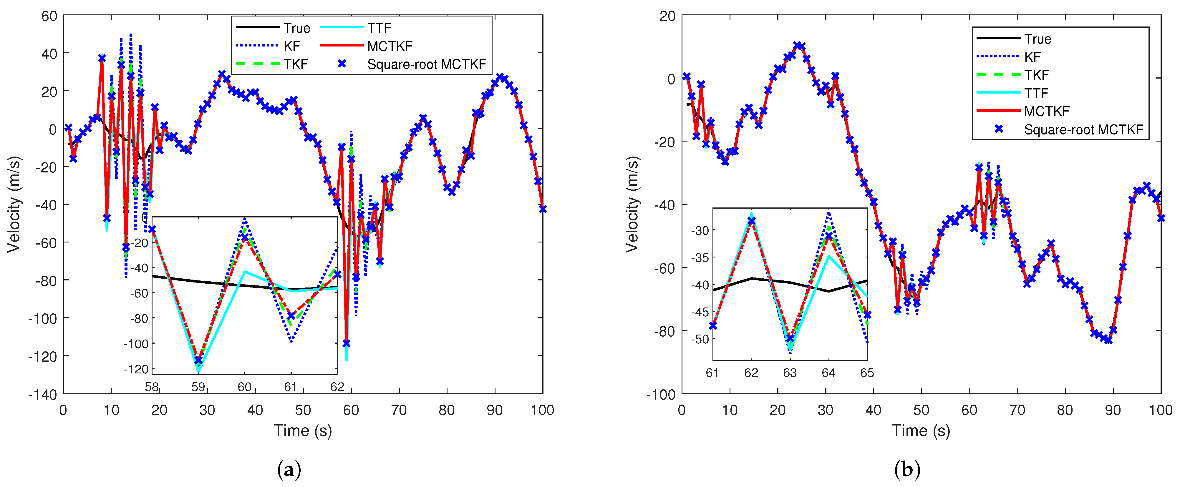
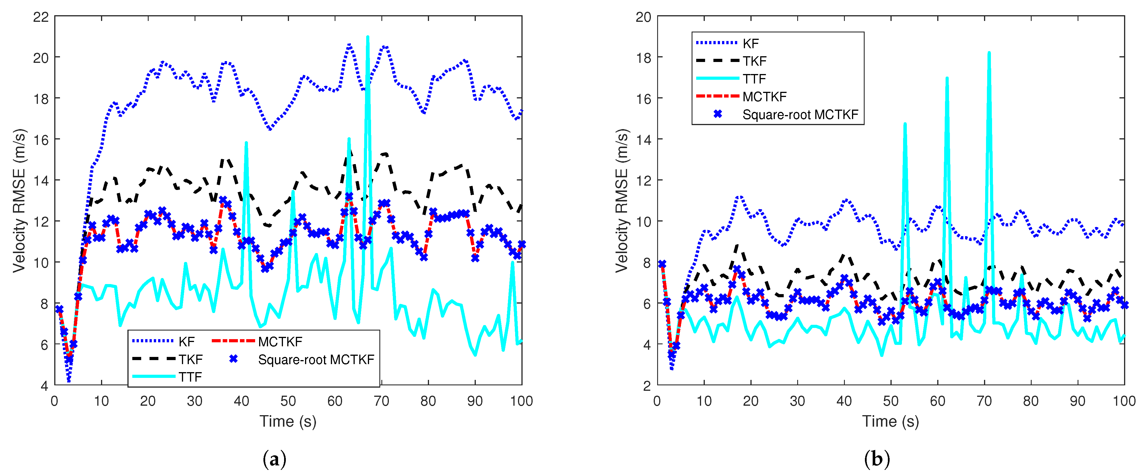
The true velocity of the target and the results of its estimation in a single trial are given in Figure 1, which shows that the proposed MCTKF and its square-root form perform better than other filters. It should be noted that all filters have similar estimation results of target position. One possible reason for this is that target position can be observed. In addition, the velocity RMSEs over 500 Monte Carlo trials are shown in Figure 2. Figure 2 shows that the MCTKF and its square-root form have the same and smaller velocity RMSEs than the TKF and KF. This indicates that the MCTKF and its square-root implementation are algebraically equivalent and can effectively deal with the state estimation problem of stochastic systems with correlated and non-Gaussian noise. The estimation performance of the TKF will degrade when the system is disturbed by some heavy-tailed noise. The KF has the worst estimation performance, because the independence and Gaussian assumptions of the process noise and measurement noise required in the KF are not satisfied in this system. The TTF is also effective for non-Gaussian noise and even performs better than the MCTKF at most of the time. This is because the Student’s t-distribution can describe the system with non-Gaussian noise more accurately than the Gaussian distribution, although it does not have an analytical solution. However, the TTF exhibits poorer robustness compared to the MCTKF. As shown in Figure 1 and Figure 2, the former has a large estimation bias at some moments. A possible reason for this is that for large outliers, the TTF relies more on measurements, while the MCTKF can reduce the impact of outliers on state estimation via the parameter . Therefore, there is a trade-off between estimation accuracy and robustness when choosing which method to use.
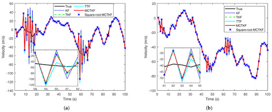
Figure 1.
True velocity and estimates in a single trial. (a) Case 1. (b) Case 2.
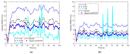
Figure 2.
Velocity RMSEs over time. (a) Case 1. (b) Case 2.
Note that the difference between the TKF and the MCTKF in Figure 2 is more significant that in Figure 1. The main reason for this is the difference in y-axis coordinate range between the two figures, and a smaller coordinate range results in more significant difference. In addition, Figure 1 is the result of a single trial, which has a certain degree of randomness, while Figure 2 is the statistical result of 500 Monte Carlo trials. This may also be a reason for this difference.
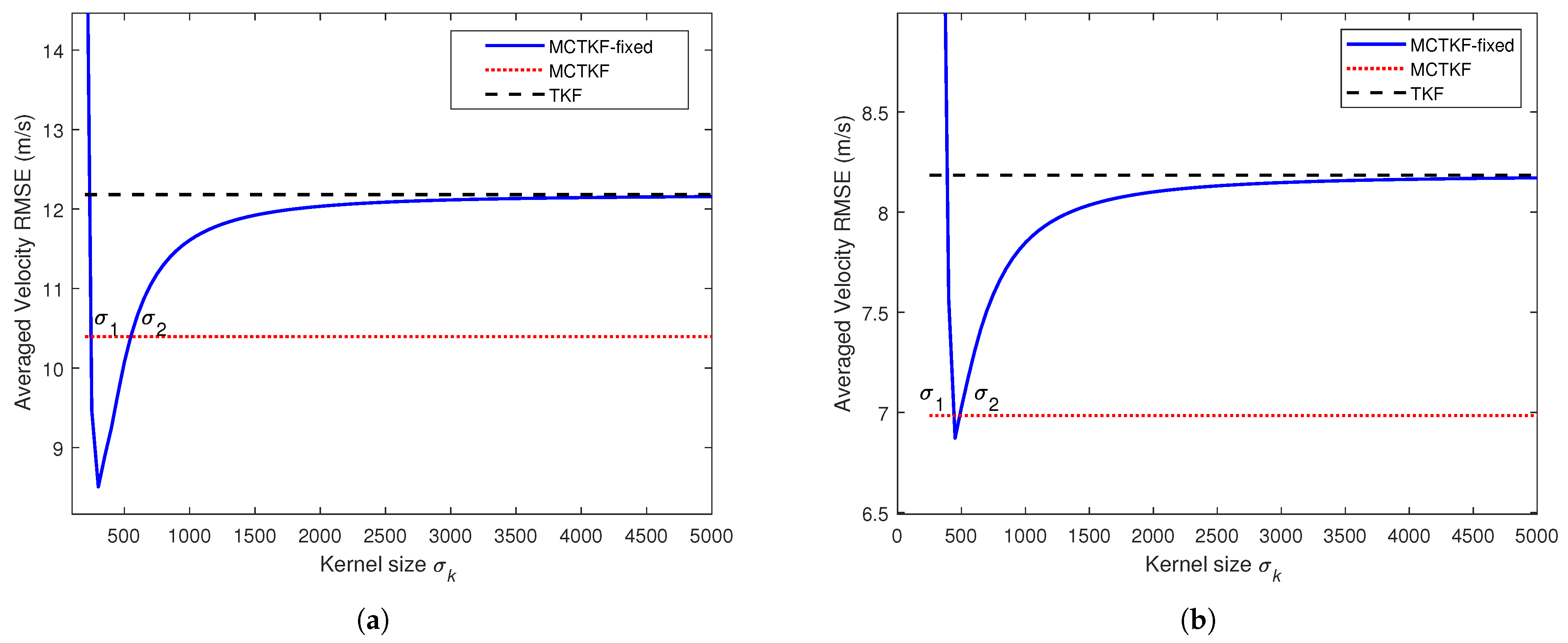
We further study the effect of the kernel size on the proposed MCTKF. To this end, the MCTKF with a fixed (MCTKF-fixed) is tested. The averaged velocity RMSEs of the MCTKF-fixed with different kernel sizes are shown in Figure 3. The results suggest that the kernel size plays a significant role in the accuracy of the MCTKF. When the kernel size is too small, the estimation accuracy of the MCTKF-fixed will severely deteriorate and even diverge. In contrast, the MCTKF-fixed will reduce to the conventional TKF as . Indeed, within a certain range, i.e., , the MCTKF-fixed performs better than the MCTKF. However, using strategy (10) for the kernel size , the MCTKF performs better than the TKF, although this strategy cannot obtain its optimal value. Therefore, the problem of the optimal kernel size selection is a very important issue in correntropy-based filters. We will focus on this issue in future research.
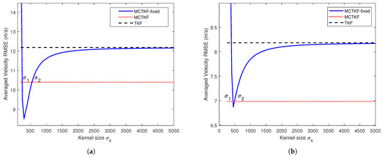
Figure 3.
Averaged velocity RMSEs of the MCTKF-fixed with different kernel size . (a) Case 1. (b) Case 2.
5.2. Linear TMC Example with Round-off Error
The square-root implementation of the MCTKF aims to improve the numerical stability of the filtering algorithm and reduce the influence of round-off errors. To further verify the robustness of the square-root MCTKF, consider the model (3) with (4) with parameters as follows:
where the parameter is utilized to simulate round-off. We assume that , but , where denotes the unit round-off error (computer-made round-off for floating-point arithmetic is often characterized by a single parameter , defined in different sources as the largest number such that either or in machine precision [38]). Two cases are considered for the system in the presence of non-Gaussian noise.
Case 1: The process noise is Gaussian noise disturbed by shot noise, and the shot noise occurs with a probability of , i.e.,
where , and the shot noise is generated by . The symbol is a Matlab instruction that an integer is randomly returned from the uniform discrete distribution of interval .
Case 2: The process noise is Gaussian mixture noise given by
where , , and .
The MCTKF and the square-root MCTKF are tested for comparative study. We conduct 100 Monte Carlo trials on various ill-conditioned parameter values . For the MCTKF, the source of the difficulty lies in the inversion of the matrix . More precisely, even though the rank of the observation matrix is (i.e., ), the matrix becomes severely ill-conditioned as , i.e., approaches the machine precision limit. The averaged RMSEs and the CPU time of a single trial are shown in Table 4.
Table 4.
RMSE results and average CPU time in the presence of shot and Gaussian mixture noises in Case 1 and Case 2, respectively.
By analyzing the results given in Table 4, we can explore the numerical behavior of each filter when the ill-conditioned problem grows. Specifically, when , both two filters perform well, and have the same RMSE results. This further indicates that the square-root MCTKF is algebraically equivalent to the conventional MCTKF. With the decrease in the parameter , the RMSE results of the two filtering algorithms are no longer the same. Smaller RMSE results indicate that the square-root MCTKF is more numerically stable than the MCTKF. In particular, when and , the MCTKF diverges, but its square-root form still performs well. In addition, taking into account the computational complexity, the averaged CPU time of the square-root MCTKF is about of that of the MCTKF.
The above analysis shows that the square-root MCTKF is more numerically stable than the conventional MCTKF, and can significantly reduce the influence of round-off errors.
5.3. Nonlinear Bearing-Only Multi-Target Tracking Example in the Presence of Non-Gaussian Noise
In this section, a bearing-only multi-target tracking example is provided to verify the effectiveness of the proposed strategy in dealing with correlated non-Gaussian noise. In multi-target tracking, data association is the main difficulty due to the uncertainties in target birth and death, clutter, and miss-detection. Interestingly, random finite set-based multi-target filtering methods [50] deal with the multi-target tracking problem from the perspective of set value estimation, avoiding the data association process. Therefore, we use the multi-Bernoulli (MB) filtering framework [43] to address the multi-tracking problem, in which the extended Kalman filter (EKF), the extended triplet Kalman filter (ETKF), and the maximum correntropy extended triplet Kalman filter (MCETKF) are tested, due to nonlinear bearing measurements.
There are a total number of 10 targets in the surveillance region . Each target moves at an approximately constant turn rate, but the turn rate is time-varying. Let the target state be , where and are the target position and velocity, respectively. Hence, the state transition model is
where
is the process noise, is the angular acceleration, and s is the sampling time. Therefore, the transformation model of the hidden state is
Both and are white noise and independent of each other. They are assumed non-Gaussian and follow a t-distribution. Let and , where denotes a t-distribution with mean , scale matrix , and degree of freedom . The t-distribution is the most commonly used heavy-tailed distribution. The parameters are set as follows: and , where , , and .
Two sensors are used to observe targets, and the measurement equation is
where denotes the position of the ith sensor, with , and is the measurement noise, with , , , and . Outliers in sensor measurements are also considered. That is, at time , the scale matrix of sensor measurement noise is with probability 0.5, or with probability 0.5. The total simulation time is 100 s. Each sensor moves at a constant velocity, and their positions shown in Figure 4a are set as follows:
The detection probability of target is . Clutter is modeled as a Poisson distribution with density over the surveillance region (that is, an average of 2 pieces of clutter per scan). Note that bearing-only target tracking is sensitive to clutter, and high clutter density leads to high false alarms. Range-and-bearing tracking is suitable for scenes with higher clutter density.
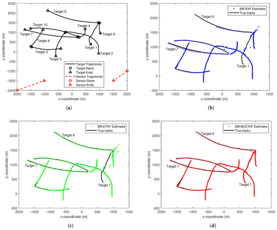
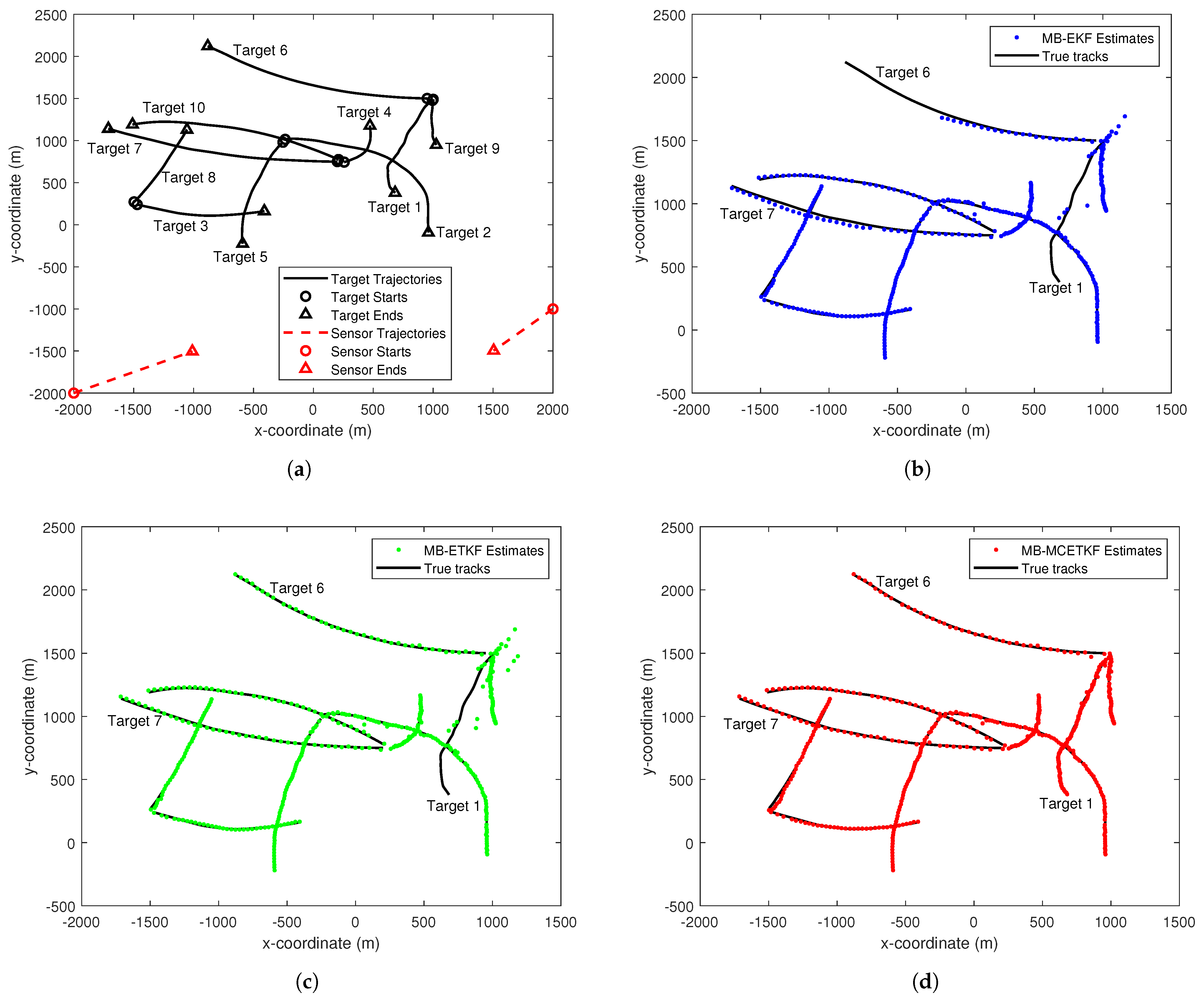
Figure 4.
The estimated results by different filters. (a) True trajectories of targets and sensors. (b) MB-EKF estimated result. (c) MB-ETKF estimated result. (d) MB-MCETKF estimated result.
Under the MB filtering framework [43], the EKF, the ETKF, and the MCETKF are tested. For the MB-ETKF and the MB-MCETKF, the birth process is a multi-Bernoulli random finite set with density , where existing probabilities are , , and corresponding probability density functions are , where the parameters are
The prior knowledge of process noise is assumed as
and the prior knowledge of measurement noise is assumed as . For the MB-EKF, all parameters are the same as those in the MB-ETKF and MB-MCETKF, except for the ignored auxiliary variable turn rate , and the turn rate in is a constant with . The survival probability of a target is .
The true trajectories of targets and sensors in a single trial are shown in Figure 4a. The estimated results of target states by the MB-EKF, the MB-ETKF, and the MB-MCETKF are given in Figure 4b–d, respectively. Intuitively, The MB-EKF and the MB-ETKF perform poorly because some targets are lost during the tracking process, such as target 1 and target 6 in Figure 4b, and target 1 in Figure 4c. The main reason for this is that both are derived using the MMSE criterion under the assumption of Gaussian noise, and the MMSE only uses the second-order term of the innovation. They easily mistake outliers originated from targets as false-alarm targets, resulting in target loss. Moreover, several false-alarm estimations appear in Figure 4b,c. The main reason for this may be that the measurement outliers near the target state can easily make the target state estimation worse, although both filters have a certain robustness toward measurement outliers. In terms of details, a significant estimation bias gradually appears over time in both target 6 and 7 shown in Figure 4b. The main reason for this is that the MB-EKF does not consider the turning rate of a target, which is time-varying over time. The proposed MB-MCETKF shows better estimation performance than the other two filters, does not suffer from target loss and false alarms, and can accurately estimate the states of each target. The main reasons for this include: first, the TMC model is more accurate and takes into account the turning rate of a target via an auxiliary variable; and second, the proposed algorithm adopts the correntropy criterion, instead of the MMSE criterion, and shows better robustness toward outliers by utilizing higher-order information of the innovation.
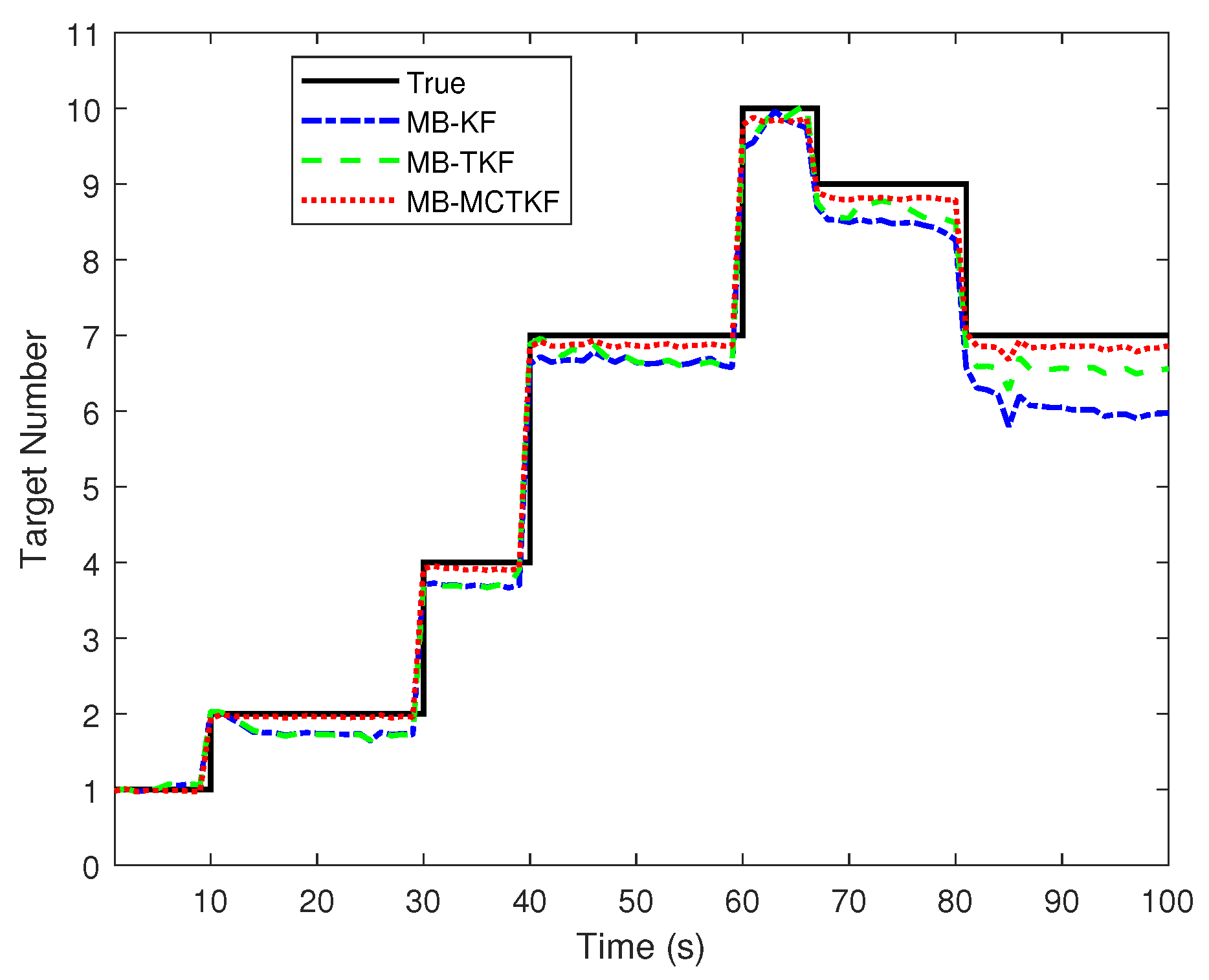
Figure 5 shows target number estimation results of different filters over 500 Monte Carlo trials. Figure 5 shows that the target number estimation of the MB-ETKF is almost same as that of the MB-EKF in the initial state, but worse than that of the MB-MCETKF. The main reason for this is that both are derived using the MMSE criterion under an assumption of Gaussian noise, and the MMSE only uses the second-order term of the innovation. They easily mistake outliers as false-alarm targets, resulting in an underestimation of target number. As time goes by, the target number estimation of the MB-EKF becomes worse than that of the MB-ETKF. The main reason for this is that the turning rate is not considered in the MB-EKF, resulting in a more inaccurate predicted state of a target, which will further reduce its robustness toward outliers. The target number estimation of the MB-MCETKF is more accurate than that of the other two filters, mainly because the former is derived by using correntropy criteria, which utilizes not only second-order but also higher-order information of the innovation, and thus, has stronger resistance toward outliers than the other two filters. Note that the MB-MCETKF can only reduce the influence of outliers to a certain extent, but cannot completely eliminate it. Therefore, large outliers may also be regarded as false alarms, resulting in an estimate of the number of targets slightly lower than the true number of targets.
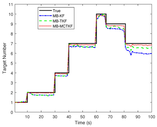
Figure 5.
Target number estimates.
To further compare the performance of the algorithms, the most popular optimal subpattern assignment (OSPA) distance for multi-target tracking is used as a metric [43]. This takes into account both the number and states of targets. Assume and , where X and are the true and estimated finite sets of targets, respectively. Let , where is the truncation distance and is the Euclidean norm, denotes the set of permutations over . For , the OSPA distance is defined by
if , and if .
The OSPA distances (where and ) of different filters over 500 Monte Carlo trials are shown in Figure 6. Figure 6 shows that its smaller OSPA distance indicates that the MB-MCETKF performs better than the other two filters, since the former can more accurately estimate the states and number of targets, shown in Figure 4 and Figure 5, respectively. In the initial stage, the MB-EKF and the MB-ETKF have similar OSPA distances and similar target number estimation results shown in Figure 5, which indicates that the former can also accurately estimate the states of targets, although it does not consider the turning rate. The main reason for this is that the initial turning rate is set to 0 rad/s in the true scenario. As time goes by, the OSPA distance of the MB-EKF becomes worse than that of the MB-ETKF. The main reasons for this include that the MB-EKF has a worse target number estimation shown in Figure 5 and its target state estimation shown in Figure 4b also becomes worse; for example, there is significant estimation bias in Target 6 and Target 7.
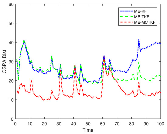
Figure 6.
OSPA distances.
The average CPU time of single-step running of each filtering algorithm is given in Table 5. It can be seen that the MB-MCETKF has almost identical CPU time to the MB-ETKF. However, because the former requires additional calculation time for the parameter (step 2, in Proposition 2), it takes slightly more CPU time. Compared to the other two filters, the MB-EKF takes the least CPU time. The main reason for this is that lower-dimensional matrix takes less computing time during the inversion operation. In this example, the state dimension in the MB-EKF is 4, which is smaller than the state dimension of 5 in the other two filters, resulting in the former taking less computational time.
Table 5.
Average CPU time of single-step running of each filtering algorithm.
6. Conclusions
In this paper, a new filter called the MCTKF is developed to address the filtering problem of stochastic systems with correlated and non-Gaussian noise. In this filter, the linear TMC model is employed to formulate the correlated relationship of stochastic systems, and the MC criterion, instead of the MMSE, is adopted to deal with non-Gaussian noise, as the former can use not only second-order but also higher-order statistics of the innovation. Furthermore, a square-root implementation of the MCTKF is designed using QR decomposition to improve the numerical stability with respect to round-off errors. Although the two filters are algebraically equivalent, simulation results show that the square-root algorithm is more numerically stable than the MCTKF for ill-conditioned problems. Both filters have simple forms, which facilitate their practical application. Numerical examples show the effectiveness of the proposed algorithms, including the nonlinear extension of the MCTKF via a bearing-only multi-target tracking example in the presence of non-Gaussian noise.
In addition, our results show that kernel size plays an important role in the two filters. Simulation results show that the adaptive kernel size selection method adopted in this paper is an effective strategy. However, it is not optimal and there is room for improvement. Therefore, the issue of optimal kernel size selection needs to be further studied.
Author Contributions
Conceptualization, G.Z. and L.Z.; methodology, G.Z. and X.Z.; software, validation, G.Z., S.D. and M.Z.; formal analysis, G.Z and F.L.; investigation; resource; data curation, G.Z. and X.Z.; writing—original draft preparation, G.Z.; review and editing, G.Z. and L.Z.; visualization, G.Z., S.D. and M.Z.; supervision, F.L.; project administration; funding acquisition, G.Z. and F.L. All authors have read and agreed to the published version of the manuscript.
Funding
This research was funded by the National Natural Science Foundation of China under Grants 62103318 and 62173266, and the Special Fund for Basic Research Funds of Central Universities (Humanities and Social Sciences) under Grant 300102231627.
Data Availability Statement
The data that support the findings of this study are available from the corresponding author upon reasonable request.
Conflicts of Interest
The authors declare no conflict of interest.
References
- Bar-Shalom, Y.; Li, X.R.; Kirubarajan, T. Estimation with Applications to Tracking and Navigation: Theory, Algorthims and Software; Wiley: New York, NY, USA, 2001. [Google Scholar]
- Jiang, M.; Guo, S.; Luo, H.; Yao, Y.; Cui, G. A Robust Target Tracking Method for Crowded Indoor Environments Using mmWave Radar. Remote Sens. 2023, 15, 2425. [Google Scholar] [CrossRef]
- Zandavi, S.M.; Chung, V. State Estimation of Nonlinear Dynamic System Using Novel Heuristic Filter Based on Genetic Algorithm. Soft Comput. 2019, 23, 5559–5570. [Google Scholar] [CrossRef]
- Lan, J.; Li, X.R. Nonlinear Estimation Based on Conversion-Sample Optimization. Automatica 2020, 121, 109160. [Google Scholar] [CrossRef]
- Zhang, G.; Lan, J.; Zhang, L.; He, F.; Li, S. Filtering in Pairwise Markov Model with Student’s t Non-Stationary Noise with Application to Target Tracking. IEEE Trans. Signal Process. 2021, 69, 1627–1641. [Google Scholar] [CrossRef]
- Kalman, R.E. A New Approach to Linear Filtering and Prediction Problems. J. Basic Eng. 1960, 82, 35–45. [Google Scholar] [CrossRef]
- An, D.; Zhang, F.; Yang, Q.; Zhang, C. Data Integrity Attack in Dynamic State Estimation of Smart Grid: Attack Model and Countermeasures. IEEE Trans. Autom. Sci. Eng. 2022, 19, 1631–1644. [Google Scholar] [CrossRef]
- Wu, W.R.; Chang, D.C. Maneuvering Target Tracking with Colored Noise. IEEE Trans. Aerosp. Electron. Syst. 1996, 32, 1311–1320. [Google Scholar]
- Saha, S.; Gustafsson, F. Particle Filtering with Dependent Noise Processes. IEEE Trans. Signal Process. 2012, 60, 4497–4508. [Google Scholar] [CrossRef]
- Li, W.; Jia, Y.; Du, J.; Zhang, J. PHD Filter for Multi-Target Tracking with Glint Noise. Signal Process. 2014, 94, 48–56. [Google Scholar] [CrossRef]
- Huang, Y.; Zhang, Y.; Li, N.; Wu, Z.; Chambers, J.A. A Novel Robust Student’s t-Based Kalman Filter. IEEE Trans. Aerosp. Electron. Syst. 2017, 53, 1545–1554. [Google Scholar] [CrossRef]
- Roth, M.; Özkan, E.; Gustafsson, F. A Student’s t Filter for Heavy Tailed Process and Measurement Noise. In Proceedings of the IEEE International Conference on Acoustics, Speech and Signal Processing, Vancouver, BC, Canada, 26–31 May 2013; pp. 5770–5774. [Google Scholar]
- Pieczynski, W.; Desbouvries, F. Kalman Filtering Using Pairwise Gaussian Models. In Proceedings of the IEEE International Conference on Acoustics, Speech, and Signal Processing, ICASSP 2003, Hong Kong, China, 6–10 April 2003; pp. 57–60. [Google Scholar]
- Pieczynski, W. Pairwise Markov Chains. IEEE Trans. Pattern Anal. Mach. Intell. 2003, 25, 634–639. [Google Scholar] [CrossRef]
- Némesin, V.; Derrode, S. Robust Blind Pairwise Kalman Algorithms Using QR Decompositions. IEEE Trans. Signal Process. 2013, 61, 5–9. [Google Scholar] [CrossRef]
- Zhang, G.H.; Han, C.Z.; Lian, F.; Zeng, L.H. Cardinality Balanced Multi-target Multi-Bernoulli Filter for Pairwise Markov Model. Acta Autom. Sin. 2017, 43, 2100–2108. [Google Scholar]
- Petetin, Y.; Desbouvries, F. Bayesian Multi-Object Filtering for Pairwise Markov Chains. IEEE Trans. Signal Process. 2013, 61, 4481–4490. [Google Scholar] [CrossRef]
- Ait-El-Fquih, B.; Desbouvries, F. Kalman Filtering in Triplet Markov Chains. IEEE Trans. Signal Process. 2006, 54, 2957–2963. [Google Scholar] [CrossRef]
- Lehmann, F.; Pieczynski, W. Reduced-Dimension Filtering in Triplet Markov Models. IEEE Trans. Autom. Control 2021, 67, 605–617. [Google Scholar] [CrossRef]
- Lehmann, F.; Pieczynski, W. Suboptimal Kalman Filtering in Triplet Markov Models Using Model Order Reduction. IEEE Signal Process. Lett. 2020, 27, 1100–1104. [Google Scholar] [CrossRef]
- Petetin, Y.; Desbouvries, F. Exact Bayesian Estimation in Constrained Triplet Markov Chains. In Proceedings of the IEEE International Workshop on Machine Learning for Signal Processing (MLSP), Reims, France, 21–24 September 2014; pp. 1–16. [Google Scholar]
- Ait El Fquih, B.; Desbouvries, F. Kalman Filtering for Triplet Markov Chains: Applications and Extensions. In Proceedings of the IEEE International Conference on Acoustics, Speech and Signal Processing, ICASSP, Philadelphia, PA, USA, 23–23 March 2005; Volume IV, pp. 685–688. [Google Scholar]
- Izanloo, R.; Fakoorian, S.A.; Yazdi, H.S.; Simon, D. Kalman Filtering Based on the Maximum Correntropy Criterion in The Presence of Non–Gaussian Noise. In Proceedings of the 2016 Annual Conference on Information Science and Systems (CISS), Princeton, NJ, USA, 16–18 March 2016; pp. 500–505. [Google Scholar]
- Zhu, J.; Xie, W.; Liu, Z. Student’s t-Based Robust Poisson Multi-Bernoulli Mixture Filter under Heavy-Tailed Process and Measurement Noises. Remote Sens. 2023, 15, 4232. [Google Scholar] [CrossRef]
- Bilik, I.; Tabrikian, J. MMSE-Based Filtering in Presence of Non-Gaussian System and Measurement Noise. IEEE Trans. Aerosp. Electron. Syst. 2010, 46, 1153–1170. [Google Scholar] [CrossRef]
- Shan, C.; Zhou, W.; Jiang, Z.; Shan, H. A New Gaussian Approximate Filter with Colored Non-Stationary Heavy-Tailed Measurement Noise. Digit. Signal Process. 2021, 122, 103358. [Google Scholar] [CrossRef]
- Zheng, F.; Derrode, S.; Pieczynski, W. Semi-supervised optimal recursive filtering and smoothing in non-Gaussian Markov switching models. Signal Process. 2020, 171, 107511. [Google Scholar] [CrossRef]
- Pieczynski, W. Exact Filtering in Conditionally Markov Switching Hidden Linear Models. C. R. Math. 2011, 349, 587–590. [Google Scholar] [CrossRef]
- Abbassi, N.; Benboudjema, D.; Derrode, S.; Pieczynski, W. Optimal filter approximations in conditionally Gaussian pairwise Markov switching models. IEEE Trans. Autom. Control 2014, 60, 1104–1109. [Google Scholar] [CrossRef]
- Gorynin, I.; Derrode, S.; Monfrini, E.; Pieczynski, W. Fast filtering in switching approximations of nonlinear Markov systems with applications to stochastic volatility. IEEE Trans. Autom. Control 2016, 62, 853–862. [Google Scholar] [CrossRef]
- Kotecha, J.; Djuric, P. Gaussian Sum Particle Filtering. IEEE Trans. Signal Process. 2003, 51, 2602–2612. [Google Scholar] [CrossRef]
- Liu, X.; Qu, H.; Zhao, J.; Yue, P. Maximum Correntropy Square-Root Cubature Kalman Filter with Application to SINS/GPS Integrated Systems. ISA Trans. 2018, 80, 195–202. [Google Scholar] [CrossRef] [PubMed]
- Liu, W.; Pokharel, P.P.; Príncipe, J.C. Correntropy: Properties and Applications in Non–Gaussian Signal Processing. IEEE Trans. Signal Process. 2007, 55, 5286–5298. [Google Scholar] [CrossRef]
- Wang, D.; Zhang, H.; Huang, H.; Ge, B. A Redundant Measurement-Based Maximum Correntropy Extended Kalman Filter for the Noise Covariance Estimation in INS/GNSS Integration. Remote Sens. 2023, 15, 2430. [Google Scholar] [CrossRef]
- Liao, T.; Hirota, K.; Wu, X.; Shao, S.; Dai, Y. A Dynamic Self-Tuning Maximum Correntropy Kalman Filter for Wireless Sensors Networks Positioning Systems. Remote Sens. 2022, 14, 4345. [Google Scholar] [CrossRef]
- Li, X.; Guo, Y.; Meng, Q. Variational Bayesian-Based Improved Maximum Mixture Correntropy Kalman Filter for Non-Gaussian Noise. Entropy 2022, 24, 117. [Google Scholar] [CrossRef]
- Chen, B.; Liu, X.; Zhao, H.; Principe, J.C. Maximum Correntropy Kalman Filter. Automatica 2017, 76, 70–77. [Google Scholar] [CrossRef]
- Kulikova, M.V. Square-Root Algorithms for Maximum Correntropy Estimation of Linear Discrete-Time Systems in Presence of Non–Gaussian Noise. Syst. Control Lett. 2017, 108, 8–15. [Google Scholar] [CrossRef]
- Liu, X.; Qu, H.; Zhao, J.; Chen, B. State Space Maximum Correntropy Filter. Signal Process. 2017, 130, 152–158. [Google Scholar] [CrossRef]
- Liu, X.; Chen, B.; Xu, B.; Wu, Z.; Honeine, P. Maximum Correntropy Unscented Filter. Int. J. Syst. Sci. 2017, 48, 1607–1615. [Google Scholar] [CrossRef]
- Gunduz, A.; Príncipe, J.C. Correntropy as A Novel Measure for Nonlinearity Tests. Signal Process. 2009, 89, 14–23. [Google Scholar] [CrossRef]
- Cinar, G.T.; Príncipe, J.C. Hidden State Estimation Using the Correntropy Filter with Fixed Point Update and Adaptive Kernel Size. In Proceedings of the The 2012 International Joint Conference on Neural Networks (IJCNN), Brisbane, QLD, Australia, 10–15 June 2012; pp. 1–6. [Google Scholar]
- Vo, B.T.; Vo, B.N.; Cantoni, A. The Cardinality Balanced Multi-Target Multi-Bernoulli Filter and Its Implementations. IEEE Trans. Signal Process. 2009, 57, 409–423. [Google Scholar]
- Bishop, C.M. Pattern Recognition and Machine Learning; Springer: New York, NY, USA, 2006. [Google Scholar]
- Zhang, G.; Lian, F.; Han, C.; Chen, H.; Fu, N. Two Novel Sensor Control Schemes for Multi-Target Tracking via Delta Generalised Labelled Multi-Bernoulli Filtering. IET Signal Process. 2018, 12, 1131–1139. [Google Scholar] [CrossRef]
- Higham, N.J. Accuracy and Stability of Numerical Algorithms; SIAM: Philadelphia, PA, USA, 2002. [Google Scholar]
- Higham, N.J. Analysis of the Cholesky Decomposition of a Semi-Definite Matrix; Oxford University Press: Manchester, UK, 1990. [Google Scholar]
- Grewal, M.S.; Andrews, A.P. Kalman Filtering: Theory and Practice with MATLAB; John Wiley & Sons: Hoboken, NJ, USA, 2014. [Google Scholar]
- Kaminski, P.; Bryson, A.; Schmidt, S. Discrete Square Root Filtering: A Survey of Current Techniques. IEEE Trans. Autom. Control 1971, 16, 727–736. [Google Scholar] [CrossRef]
- Mahler, R.P. Advances in Statistical Multisource-Multitarget Information Fusion; Artech House: Norwood, MA, USA, 2014. [Google Scholar]

Disclaimer/Publisher’s Note: The statements, opinions and data contained in all publications are solely those of the individual author(s) and contributor(s) and not of MDPI and/or the editor(s). MDPI and/or the editor(s) disclaim responsibility for any injury to people or property resulting from any ideas, methods, instructions or products referred to in the content. |
© 2023 by the authors. Licensee MDPI, Basel, Switzerland. This article is an open access article distributed under the terms and conditions of the Creative Commons Attribution (CC BY) license (https://creativecommons.org/licenses/by/4.0/).