Abstract
Total suspended solids (TSS) and chlorophyll-a (Chl-a) are critical water quality parameters. Focusing on the Pearl River Estuary and its coastal waters, this study compared the performance of XGBoost- and BPNN-based algorithms in estimating TSS and Chl-a levels. The XGBoost-based algorithm demonstrated better performance and was then used to estimate TSS and Chl-a in the Pearl River Estuary and coastal waters from 2000 to 2021. According to our results, TSS and Chl-a were relatively high mainly in the northwest and low in the southeast. Furthermore, values were high in spring and summer and low in fall and winter, with high values emerging near the estuary of the Pearl River. In summer, a band zone with high Chl-a was observed from south of Yamen to south of Hong Kong. In terms of trends, TSS and Chl-a concentrations in the area around the Hong Kong–Zhuhai–Macao Bridge tended to decrease from 2000 to 2021. As the construction of the bridge began, changes in water flow caused by the bridge piers and artificial islands were influenced, the change in the rate of TSS in the west area of the bridge was greater than 0, and the TSS in the upstream area of the west side changed from decreasing to increasing trends. Concerning Chl-a concentrations, the change in the rate in the downstream area of the west side of the bridge was greater than 0. The study may provide a helpful example for similar estuarine and coastal waters in other coastal areas.
1. Introduction
Estuaries are hubs between river runoff and the sea, and their ecosystems are fragile [1]. The Pearl River Estuary (PRE), an eminently crucial estuarine area [2], is located in a well-developed and populous area; thus, human activities directly affect the water quality of the surrounding waters [3,4,5]. The serious potential consequences underscore the urgent need to study the water quality of the PRE and its coastal waters.
Total suspended solids (TSS) and chlorophyll-a (Chl-a) are significant water quality parameters, as they are indispensable in the evaluation of estuarian water quality [6]. The transport and accumulation of TSS may have many effects on navigation channels. For example, high concentrations can reduce phytoplankton photosynthesis [7], adversely affecting phytoplankton, fish, and benthic invertebrates [8]. For this part, Chl-a is relevant to water eutrophication and algal blooms, which have the potential to inflict serious damage upon the nearshore ecological environment [9,10,11]. Therefore, a scholarly examination of the distribution pattern and change trend in TSS, Chl-a, and other water quality parameters in estuarine areas is of paramount importance.
Due to its advantages, such as rapid information acquisition, low cost, and a broad range, remote sensing has become the primary means for monitoring water quality in many areas [12,13,14,15], as it can provide a large amount of data in real time. Another useful tool is found in machine learning algorithms, which researchers appreciate for their powerful data mining capabilities and abilities to explore deeper correspondences [16,17].
The increasing availability of remote sensing data has led to the wider use of machine learning algorithms in water quality models, promoting the use of big data in the monitoring of water quality [18,19,20,21]. Ma et al. [22] developed an algorithm based on an artificial neural network (ANN) to obtain TSS and Chl-a concentration characteristics in the PRE area from MODIS/Aqua data. Employing an algorithm based on a back propagation neural network (BPNN), Wang et al. [23] explored the impact of suspended particulate matter, orthophosphate phosphorus, and dissolved inorganic nitrogen on surrounding waters during the construction of the Hong Kong International Airport. In addition to algorithms based on neural network technology, support vector machine regression (SVR) [24,25,26], random forest regression (RFR) [27,28], and XGBoost [29] algorithms have also been applied to establish water quality models. However, further demonstrations of the feasibility of using machine learning algorithms to determine TSS and Chl-a levels in the PRE and its coastal waters from the images of different Landsat satellites are needed, as well as further investigation into how the Hong Kong–Zhuhai–Macao Bridge (HZMB) affects the water quality of the surrounding waters.
Accordingly, we set four goals in this study. Specifically, we aimed to (a) identify input bands strongly correlated with TSS and Chl-a and then establish and compare water quality models based on XGBoost and BPNN algorithms; (b) use the better performing machine learning-based algorithm to measure TSS and Chl-a in the PRE from Landsat 5/8 images; (c) explore the spatiotemporal distribution characteristics of TSS and Chl-a in the PRE from 2000 to 2021; and (d) scrutinize the influence of the HZMB on the surrounding water quality.
2. Materials and Methods
2.1. Study Area
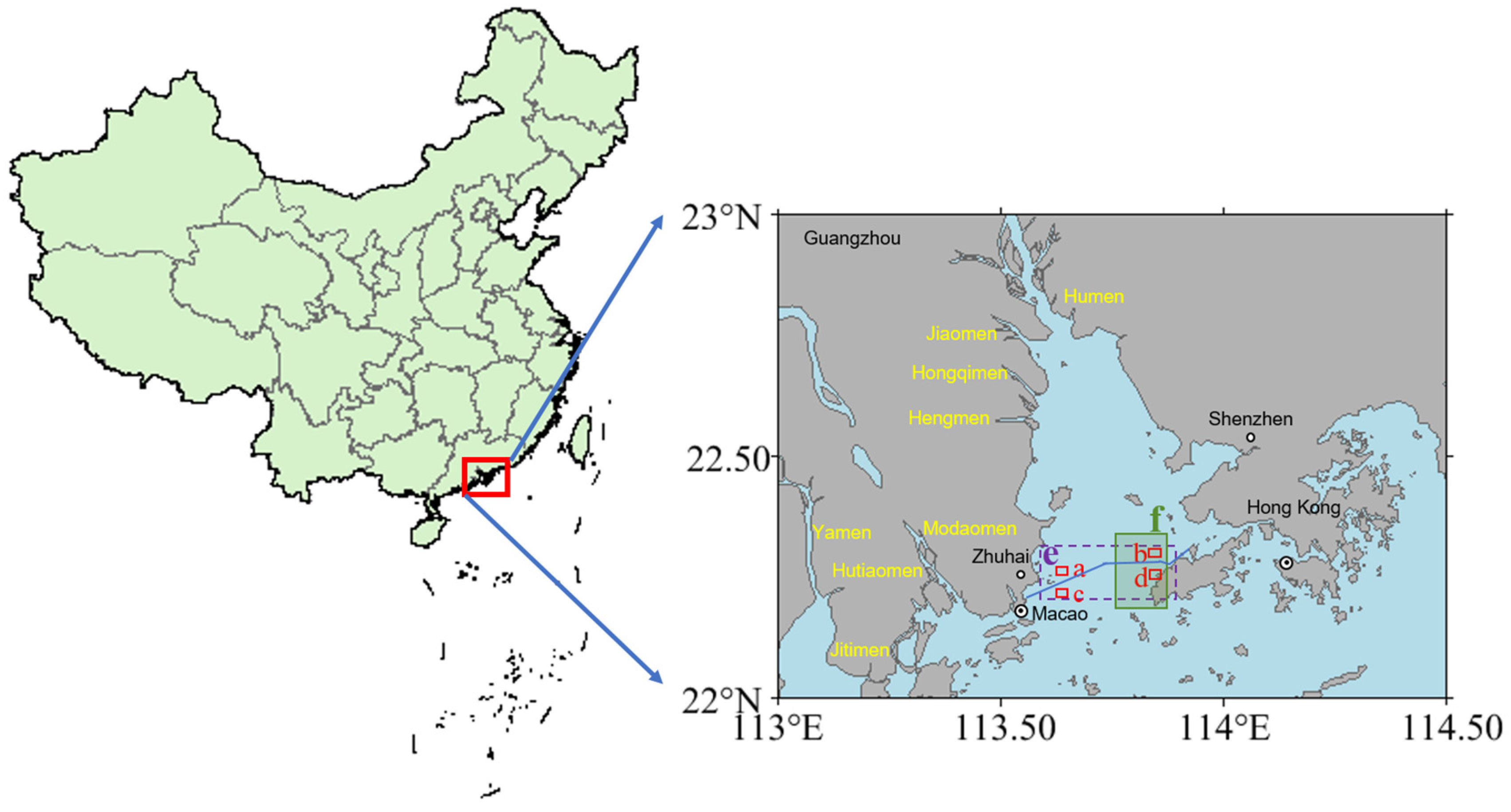
The Pearl River is the largest river system in southern China, with a total length of 2200 km. It has eight main estuaries, Humen, Jiaomen, Hongqimen, Hengmen, Modaomen, Jitimen, Hutiaomen, and Yamen, from east to west [30]. The basin area is about 4.5 × 10⁵ km2 [31], and its annual average flow can reach 3.5 × 10¹¹ m3, with an annual sediment transport of 8.87 × 10⁷ t [32]. The PRE lies in the northern part of the South China Sea and is influenced by subtropical monsoon climate [33]. The runoff in this area changes significantly with the seasons. With the rapid development of cities such as Hong Kong, Guangzhou and Shenzhen, the situation of water pollution in the PRE is serious. There is a sea-crossing bridge–tunnel project in the PRE connecting Hong Kong, Zhuhai, and Macao—the HZMB, a 55 km long construction, started in late 2009 and officially opened in 2018 [34]. There is also a national nature reserve for Chinese white dolphins in the PRE between Neilingding Island and Niutou Island [35], the core area of which covers 140 km2. In order to better analyze changes in water quality in certain areas, five specific areas, a–f, are shown in Figure 1.
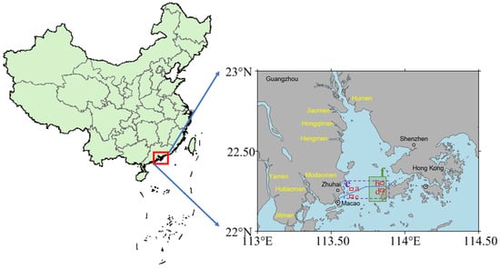
Figure 1.
Introduction to the study area (Areas a–d are square areas with an area of 4 km2 on the west side of the upper reaches, east side of the upper reaches, west side of the lower reaches and east side of the lower reaches of the HZMB. Area e is a rectangular area covering the HZMB, and area f represents the core area of the Chinese white dolphin national nature reserve in the PRE).
2.2. In Situ Data
Monthly measured TSS and Chl-a concentration data (20,791 lines) provided by the Environmental Protection Department (EPD) of Hong Kong for the years 2000–2021 were used in this study. The data were mainly measured by marine monitoring vessels equipped with Differential Global Positioning System (DGPS) at 76 water quality sampling stations in 10 water control zones and 18 offshore sheltered sites in Hong Kong. TSS and Chl-a were measured by internal analysis methods GL-PH-23 and GL-OR-34, respectively, and determined by weight method (APHA 20ed 2540D) and spectrophotometric method (APHA 22ed 10200H 2) [36], respectively, with uncertainties of ±0.5 mg/L and ±0.1 mg/m3, respectively.
2.3. Satellite Data and Preprocessing
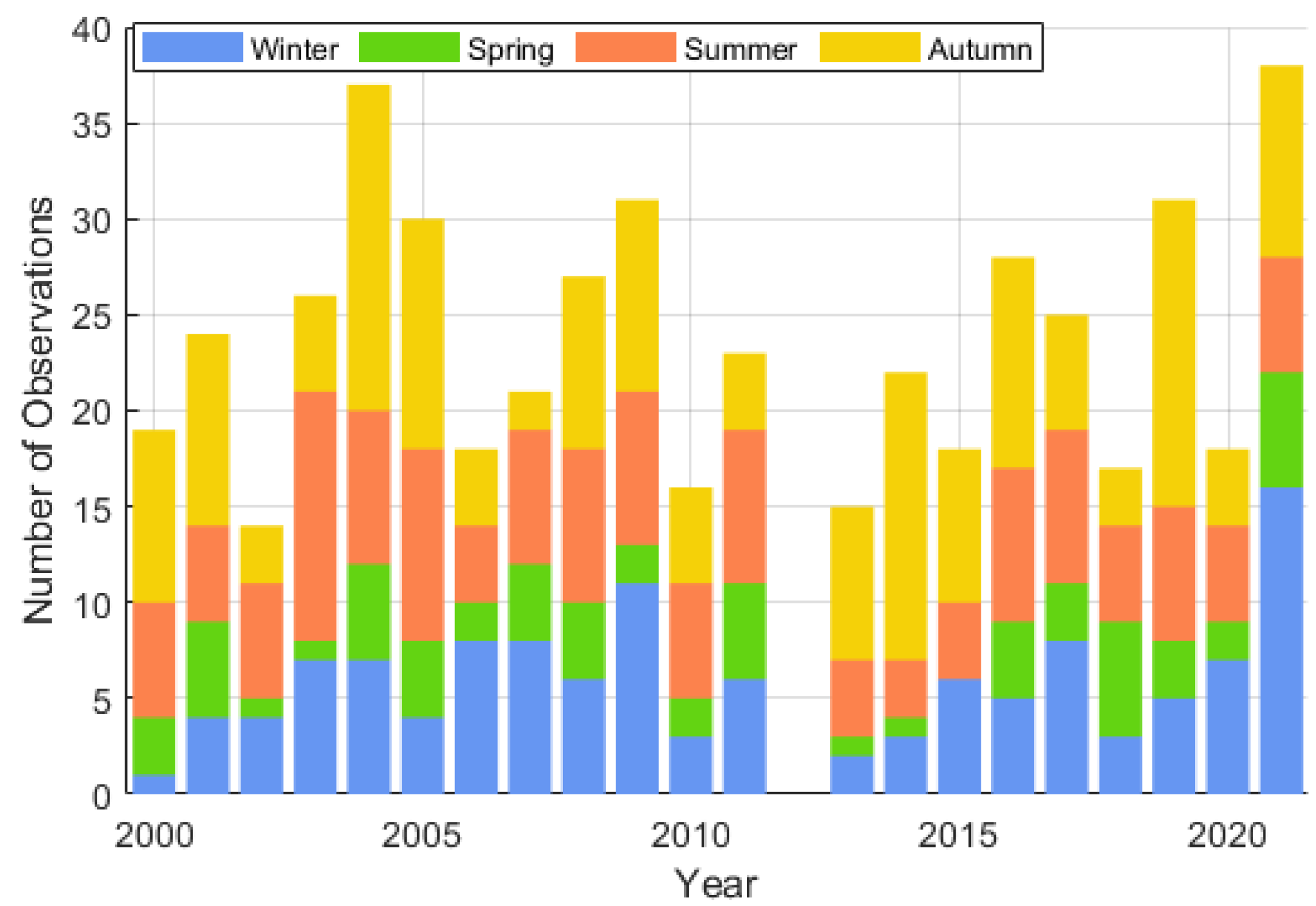
This study used L1-level satellite images of Landsat 5 TM and Landsat 8 OLI from 2000 to 2021 (bands are shown in Table 1). The data were downloaded from the official website of the United States Geological Survey (USGS). In order to ensure the coverage of the PRE and the adjacent Hong Kong region, we selected the images with the path/row numbers 122/044, 122/045, 121/044, and 121/045 and screened the images with less than 30% cloud coverage out. Finally, 292 Landsat 5 TM images and 217 Landsat 8 OLI images were retained. As shown in Figure 2, the seasonal distribution of remote sensing images shows that the number of images in autumn is greater than that in summer, and the number of images in winter is greater than that in spring, and the number of images in spring is only half of that in other seasons. The atmospheric correction of all the images was performed by ACOLITE (Generic Version 20220222.0). ACOLITE was developed by the Royal Belgian Institute of Natural Sciences (RBINS) and can output a series of parameters calculated from water reflectance [37]. In this study, non-water pixels were masked during atmospheric correction, other parameters were kept at default settings, and remote sensing reflectance (Rrs) was output.

Table 1.
Introduction of Landsat 5 TM and Landsat 8 OLI sensor parameters.
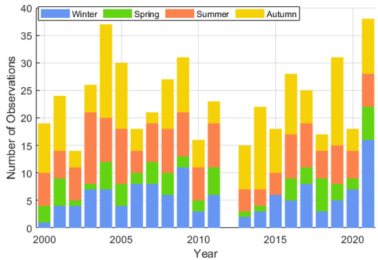
Figure 2.
The temporal distributions of all images used.
The Landsat 8 OLI sensor added a coastal aerosol band and a panchromatic band with a spatial resolution of 15 m, and a cirrus cloud band based on the Landsat 5 TM sensor. The panchromatic band is primarily used to improve resolution [23]. The band ranges of Blue, Green, Red, and NIR bands are basically the same for both sensors. To obtain a longer time series dataset, this study matched bands with similar wavelength ranges (as shown in Table 2).
Table 2.
The band numbers specified in this study.
2.4. Match-Up Analysis
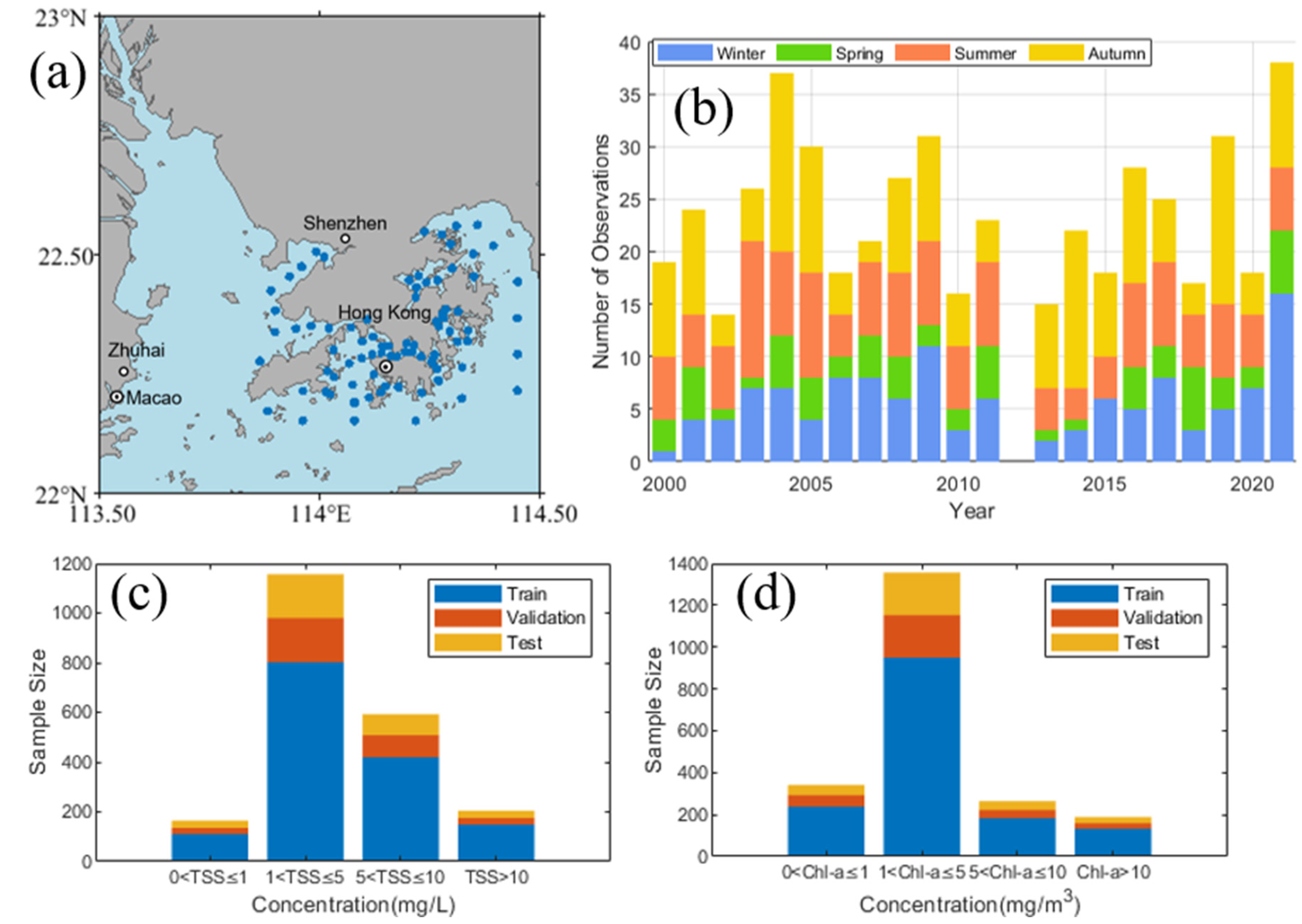
Considering the small amount of measured data, remote sensing images within 3 days before and after the measured date were selected as the images of measured sampling during data matching. In these matching images, the pixel of the remote sensing image that is closest to the measured site is found, and the other 8 pixels around it are found, with this pixel as the center. For the sake of ensuring the validity of the data, the matching is effective when at least 5 pixels in the 3 × 3-pixel box are valid, and the average reflectivity of the 9 pixels is taken as the matching value of the measured data. Finally, 2158 sets of measured and remote sensing matching data were obtained from 262 Landsat 5 TM images and 185 Landsat 8 OLI images. The matching data sets ranged from 0.1 to 79 mg/L for TSS and 0.1 to 50 mg/m3 for Chl-a. The 2158 sets of matched data pairs were randomly divided into three data sets according to the proportion of 70% training set (N = 1510), 15% testing set (N = 324), and 15% verification set (N = 324). Characteristics of matched data pairs are shown in Figure 3. The location-matched data pairs almost cover the entire sea area around Hong Kong. The time of the matched data pairs is more in autumn and winter, especially winter, but relatively less in spring and summer (December to February is winter, March to May is spring, June to August is summer, and September to November is autumn). The time of the matched data pairs can cover the four seasons of spring, summer, autumn, and winter. The TSS and Chl-a concentrations of the training, validation, and testing sets are distributed across the concentration ranges.

Figure 3.
Characteristics of matched data pairs ((a): Spatial distribution of matched data pairs; (b): The temporal distributions of matched data pairs; (c,d): Characterization of the concentration distribution of TSS/Chl-a for paired data pairs).
2.5. Modeling
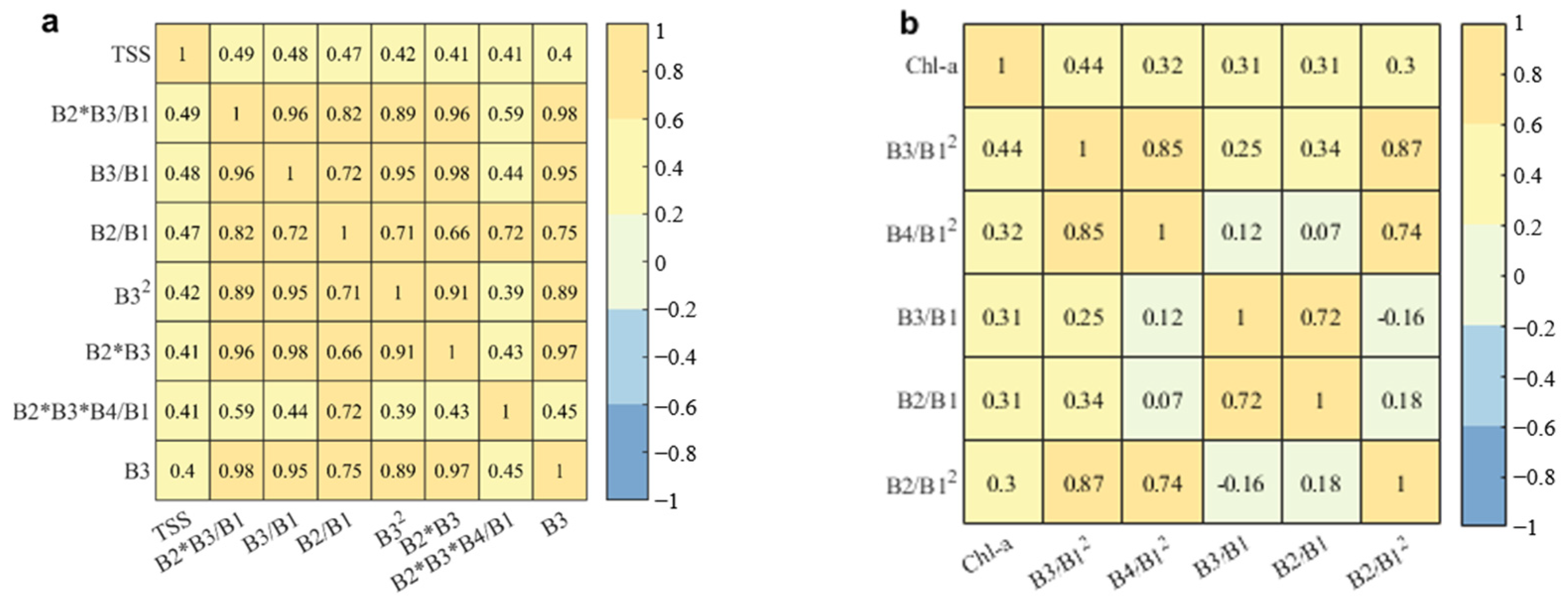
Due to the limited amount of matched data pairs, we calculated Pearson’s R coefficient of dozens of combinations of B1–B4 bands and TSS and Chl-a concentrations when selecting input bands and selected several bands with the highest correlation as input features of the machine learning model to help improve the training effect of the machine learning model. When estimating TSS, 7 band combinations with R values greater than 0.4 were selected as inputs (Figure 4a). The correlation between each band combination and Chl-a was lower. Five band combinations with R greater than 0.3, namely, B3/B12, B4/B12, B3/B1, B2/B1, and B2/B12, were selected as inputs (Figure 4b).
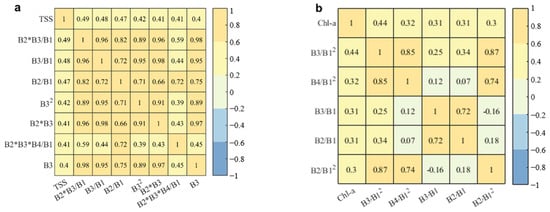
Figure 4.
Pearson’s R coefficient of each selected band (a): TSS, (b): Chl-a.
In this study, XGBoost and BPNN are selected, which belong to the machine learning algorithm based on decision tree and the machine learning algorithm based on neural network, respectively [38]. XGBoost is an enhanced integrated algorithm composed of multiple regression trees proposed by Chen and Guestrin. It reduces the complexity of the model by introducing regularization terms, so as to prevent over-fitting from reducing the computation amount [39].
When the algorithm based on XGBoost is used, estimators = 234, learning_rate = 0.03, and max_depth = 8 are set when estimating TSS, and estimators = 61 and learning_rate = 0.1 when estimating Chl-a. max_depth = 14. Retain the default values for other hyperparameters. BPNN is a multi-layer feedforward neural network trained based on error backpropagation algorithm, which can make the mean square error between the actual output value and the expected output value minimized based on gradient descent method [40]. When using BPNN-based algorithm, two BPNN algorithms with hidden layer neurons of 8 (transfer function of ‘tansig’) are constructed, respectively, when estimating TSS and Chl-a. Levenberg–Marquardt method is selected for training algorithm, so as to avoid overfitting. Set training to stop when the mean square error (MSE) curve of the verification set does not decrease for 6 consecutive iterations, and the MSE of the training set is <10−5, or the number of trainings reaches 1000.
2.6. Accuracy Evaluation
To evaluate the performance of the algorithm, this study applied the root mean square error (RMSE), root mean square log-error (RMSLE), mean absolute error (MAE), and mean percentage error (MAPE) of the water quality parameters calculated by the algorithm and the measured water quality parameters [22,41]. The calculation formulas are as follows:
where represents the estimated values, represents the measured values, and n represents the number of the match data pairs.
2.7. Summary
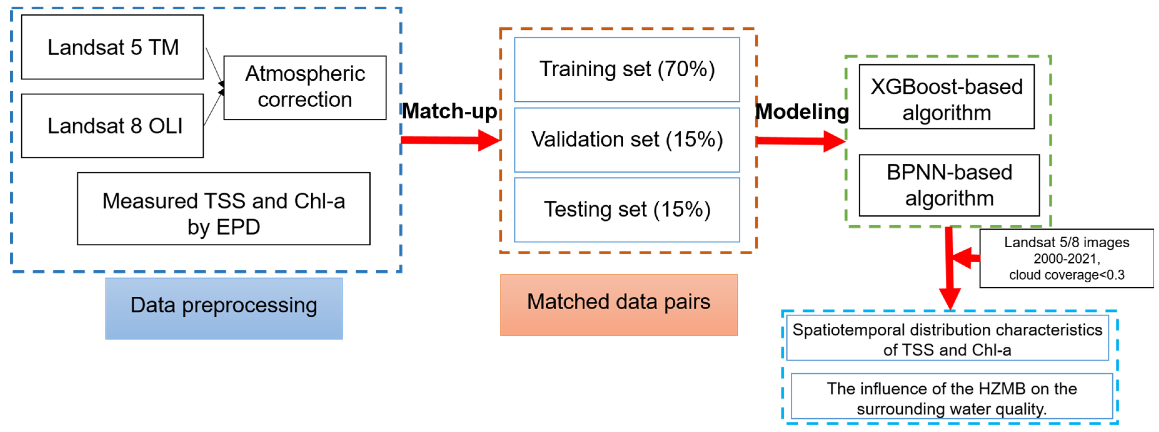
Figure 5 shows the flowchart for data processing. In summary, in this study, the Landsat 5/8 images were atmospherically corrected, and the Rrs was matched with the TSS and Chl-a data from the EPD to obtain matched data pairs, which were then divided into training set, validation set, and testing set and used to develop two algorithms based on the XGBoost and the BPNN. The better performing of the two algorithms was used to investigate the spatial and temporal distribution characteristics of TSS and Chl-a in the PRE and the impact of the HZMB on the water quality of its surrounding waters from 2000 to 2021.

Figure 5.
Flowchart of data processing.
3. Results
3.1. Evaluation of Machine Learning Algorithms
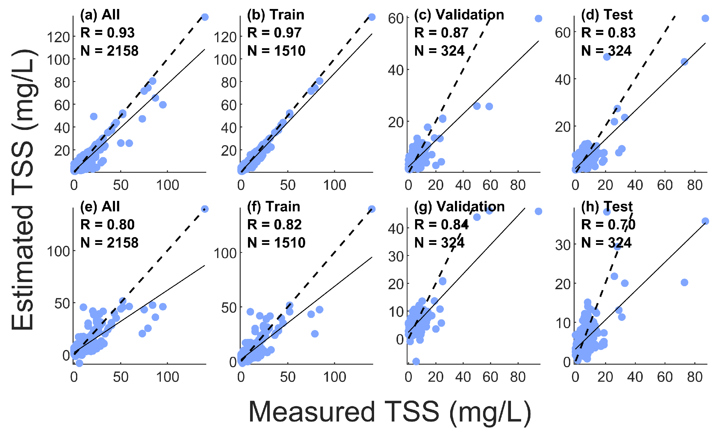
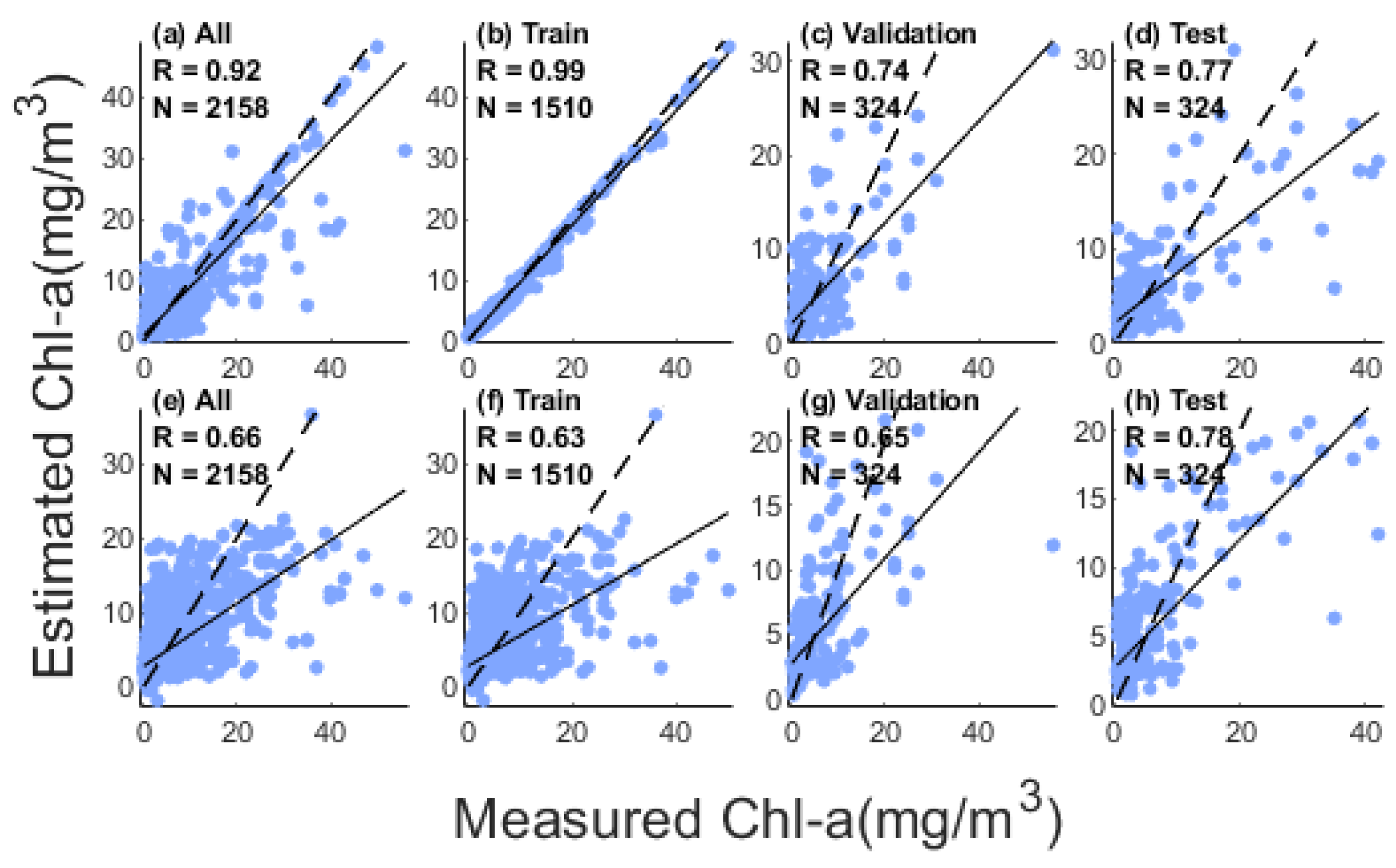
The comparison between the estimated and measured concentration of TSS and Chl-a based on XGBoost algorithm and BPNN algorithm for each data set is shown in Figure 6a–h and Figure 7a–h. The scatter between the estimated and measured concentration of all data sets is near the 1:1 line, and both algorithms have certain underestimation when estimating TSS and Chl-a. This may be due to the greater number of low values of TSS and Chl-a in the matched data pairs. The specific evaluation data of each set are shown in Table 3.
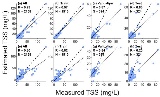
Figure 6.
Correlation between estimates and in situ concentration of TSS ((a–d) for XGBoost-based algorithm, (e–h) for BPNN-based algorithm, black dotted line for 1:1, black solid line for fitting line).
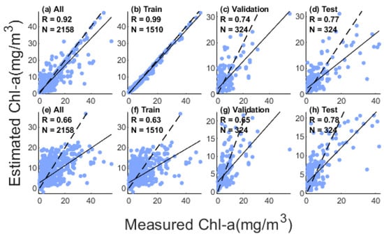
Figure 7.
Correlation between estimates and in situ concentration of Chl-a ((a–d) for XGBoost-based algorithm, (e–h) for BPNN-based algorithm, black dotted line for 1:1, black solid line for fitting line).
Table 3.
Statistical characteristics of all paired data sets, training sets, testing sets, verification sets, and evaluation indexes of TSS (unit: mg/L) and Chl-a (unit: mg/m3) estimated by the two algorithms.
For TSS estimation, XGBoost performed better than BPNN. The correlation coefficient R between the estimated and measured concentration of all data in the matched data pairs is 0.93, which is better than that of BPNN (0.79). The RMSE of the training set, verification set, and testing set of the XGBoost-based algorithm ranges from 1.88 to 4.29 mg/L, MAE ranges from 1.41 to 2.41 mg/L, and R2 ranges from 0.68 to 0.93, whereas, for the BPNN-based algorithm, the RMSE of these sets ranges from 4.08 to 5.57 mg/L, MAE ranges from 2.58 to 2.97 mg/L, and R2 ranges from 0.46 to 0.66. For Chl-a estimation, XGBoost also performs better. When the algorithm based on XGBoost is used, the R between the estimated and measured concentration ranges from 0.74 to 0.99, and the RMSE, MAE and R2 of each data set range from 0.66 to 4.37 mg/m3, 4.24 to 4.88 mg/m3, and 0.55 to 0.99, respectively. The BPNN-based algorithm produced Rs of 0.64–0.66, RMSEs of 4.37–4.47 mg/m3, MAEs of 2.43–2.56 mg/m3, and R2s of 0.40–0.57 for each data set.
Therefore, in this study, the XGBoost-based algorithms were selected to obtain the TSS and Chl-a of PRE from Landsat 5/8 images and carried out the computational analysis of the long time series.
3.2. Long-Term Water Quality in the PRE
3.2.1. Spatial Distribution
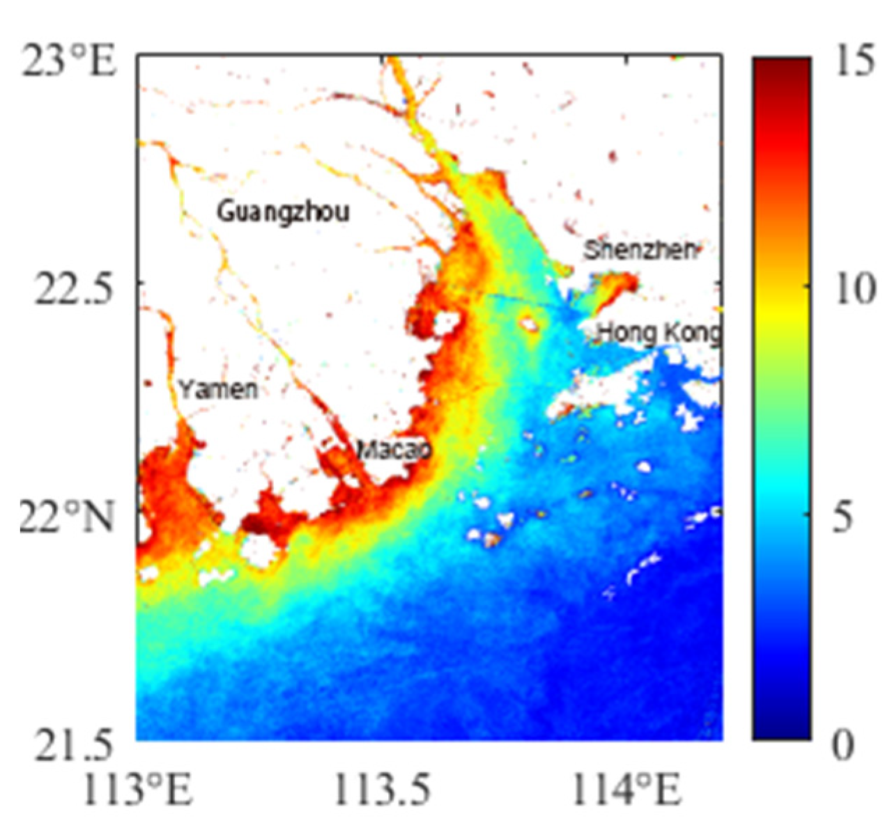
Figure 8 and Figure 9 show the average TSS and Chl-a in the PRE during 2000–2021, respectively. Both TSS and Chl-a are high in the northwest and low in the southeast, and generally decrease with the increase in the distance from the coastline. The maximum concentration of TSS appears in the surrounding waters of eight major estuaries of the Pearl River, especially in the west coast of Lingdingyang, the coastal waters south of Modaomen, and the coastal areas west of Huangmaohai. Due to the influence of the Coriolis force, the current tends to be skewed to the right, the large quantity of sediment brought by the current at the sea inlet tends to the west coast, and the suspended matter brought by the lateral inlet and the lateral shallow mouth is easy to be trapped [42]. The rapid current may lead to re-suspension when the water depth is relatively shallow, which eventually leads to the maximum TSS in these places. TSS is relatively low in the east coast of Lingdingyang, but there are also a few areas with high TSS in Shenzhen Bay and the east coast of Humen, which may be mainly related to human activities along the coast [2,43]. The spatial distribution of Chl-a in Lingdingyang is basically similar to that of TSS, but a relatively high chl-a appears in the sea area south of Yamen to the belt area north of Dandan Island south of Hong Kong. This is mainly due to the fact that a large amount of sewage brought by the Pearl River may contain a large amount of algae [44], resulting in a high Chl-a near the estuary, whereas the area farther from the shoreline tends to have lower turbidity, which enables the phytoplankton to receive more light, forming a high zonal Chl-a distribution.
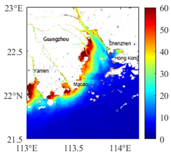
Figure 8.
Average TSS concentration for 2000–2021 period in the PRE.

Figure 9.
Average Chl-a concentration for 2000–2021 period in the PRE.
3.2.2. Seasonal Variations
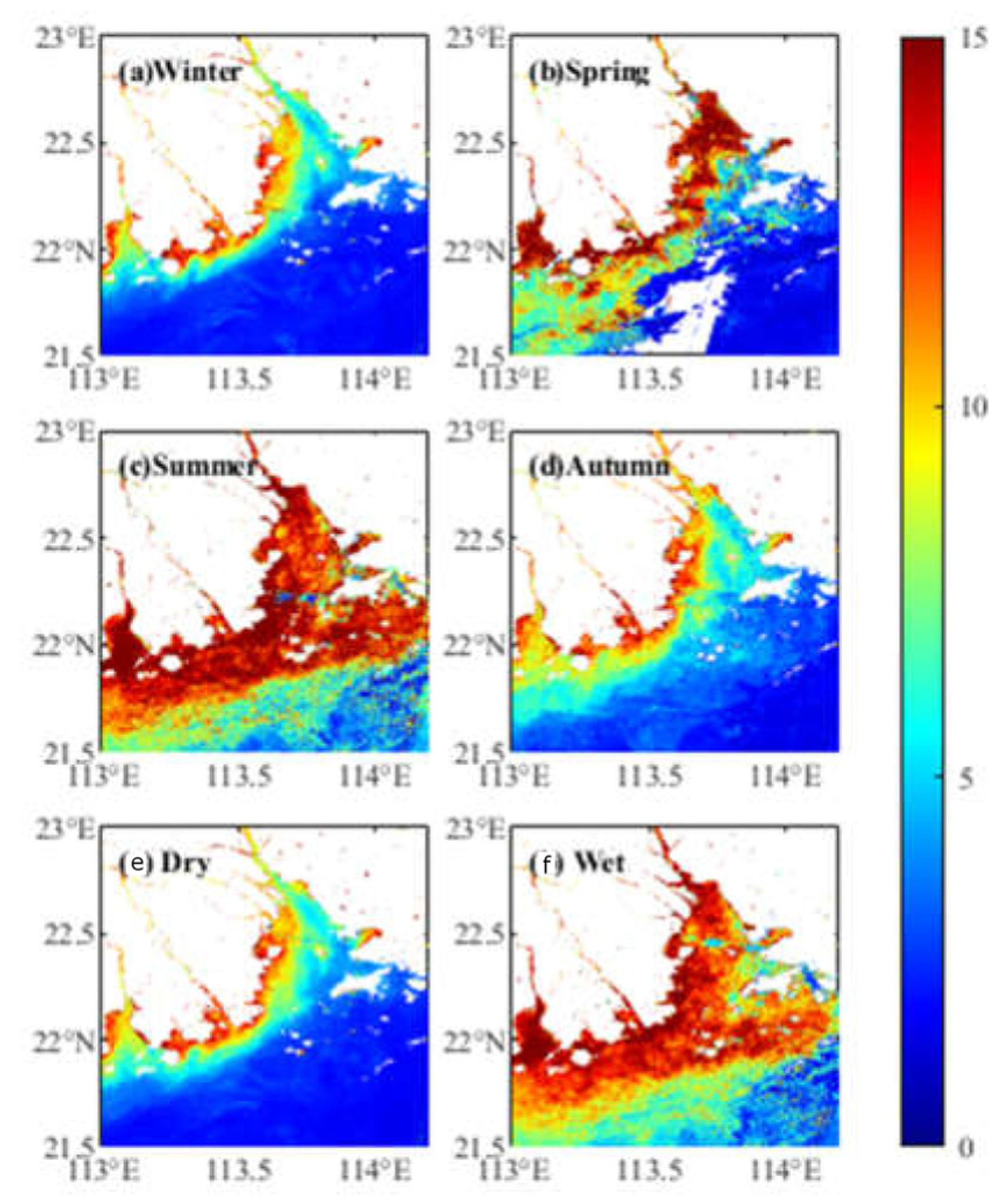
The average of TSS and Chl-a in each season, dry season, and wet season in the PRE are shown in Figure 10 and Figure 11 (the dry season is from October to March of the following year, and the wet season is from April to September). The spatial distribution of maximum and maximum concentration of TSS in each season is the same as that of the annual average concentration of TSS, and both decrease gradually from the estuary with the distance from the coastline. The TSS in spring and summer is evidently higher than that in autumn and winter, and the high TSS in spring and summer expands away from the shoreline, which is mainly influenced by the flow of the Pearl River. In spring and summer, a large sum of suspended sediment carried by the Pearl River is discharged from various estuaries, which expands the influence range of the high TSS, which can also be verified by the comparison between dry season and wet season. Chl-a also has different characteristics in different seasons and is higher in summer than in spring and higher in autumn than in winter. With the arrival of spring and summer, the upper sea temperature gradually increased, and the growth of phytoplankton accelerated [45]. Moreover, the water flow could spread the phytoplankton to further areas, making the high Chl-a distribution zone from the south of Modaomen to the north of Dandan Island, south of Hong Kong, more evident. The distribution of Chl-a in dry season and wet season also supports the influence of water flow in the estuary on this phenomenon.
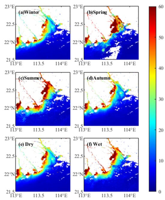
Figure 10.
The average concentration of TSS in winter (a), spring (b), summer (c), autumn (d), dry season (e), and wet season (f).

Figure 11.
The average concentration of Chl-a in winter (a), spring (b), summer (c), autumn (d), dry season (e), and wet season (f).
3.3. Impact of HZMB on Surrounding Water Quality
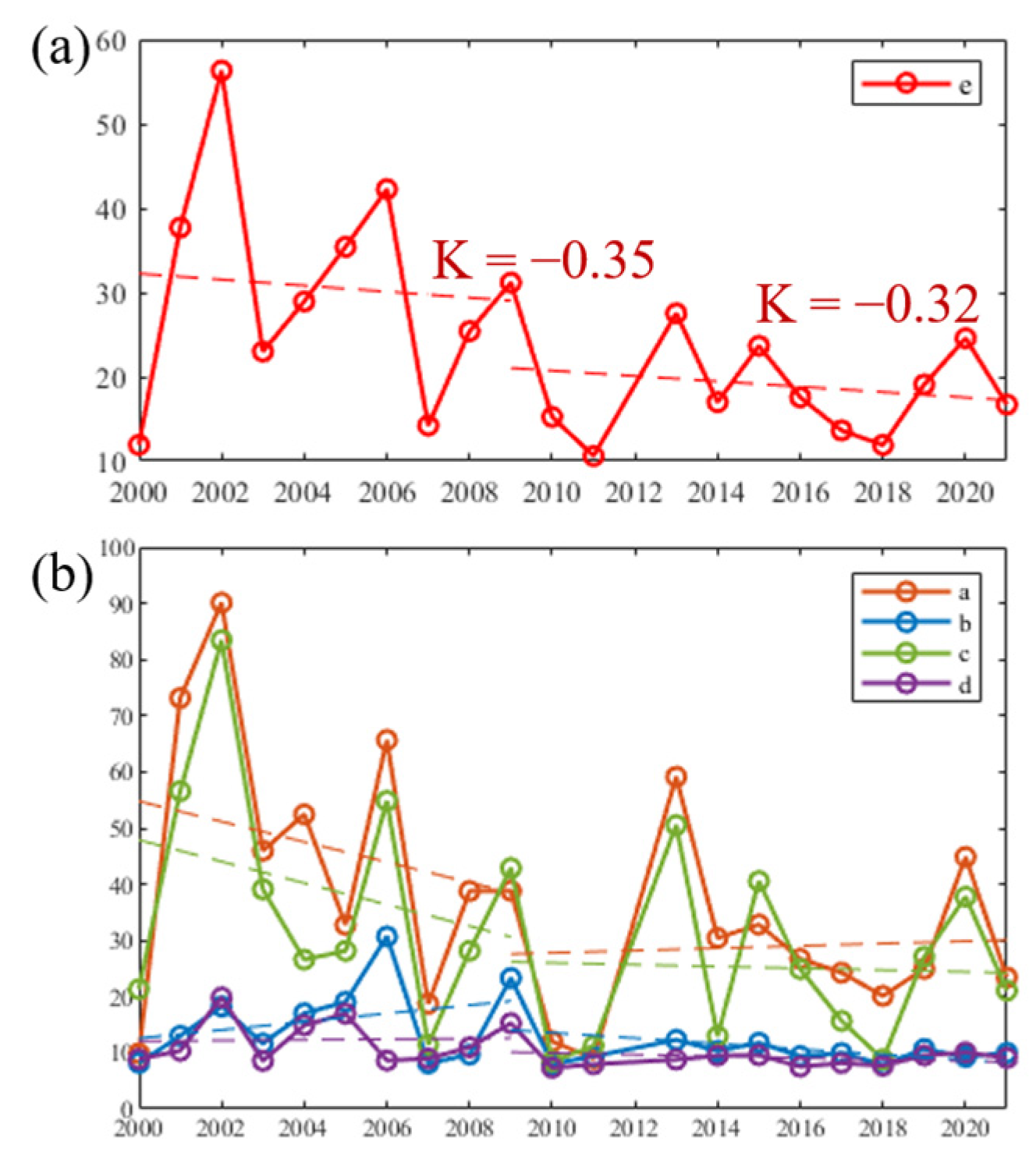
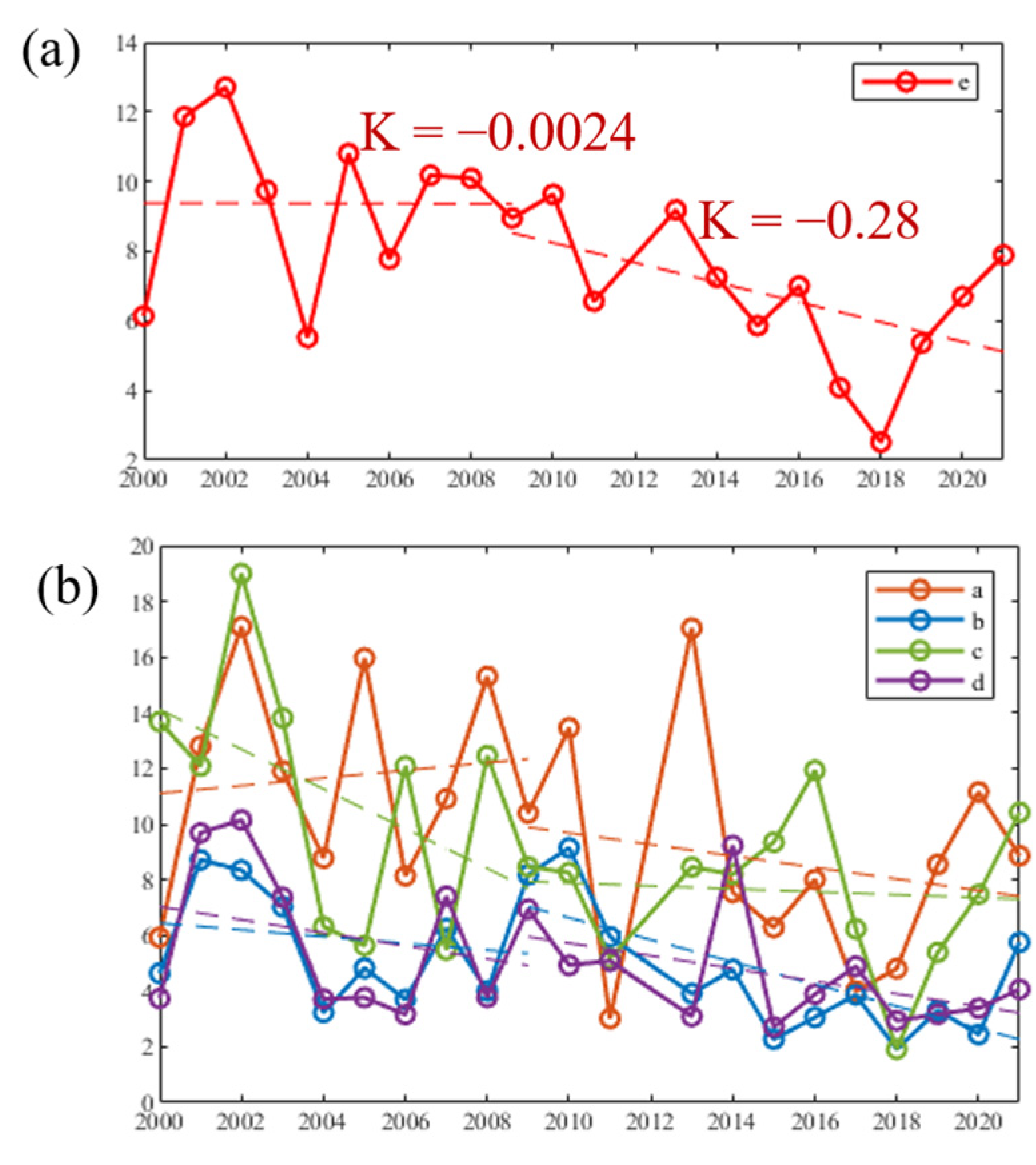
Figure 12 and Figure 13 show the changes in TSS and Chl-a concentrations in areas a-e from 2000 to 2021. For area e, which covers the whole HZMB, both TSS and Chl-a show a decreasing trend as a whole. As the erection of the HZMB officially commenced in December 2009, we divided the time into two time periods, 2000–2009 and 2009–2021. Since 2009, the decreasing trend in TSS is weakened with a rate of change greater than zero in region e, whereas the decreasing trend in Chl-a is enhanced with a rate of change less than zero. This may be due to the change in water quality within 7 km upstream and downstream of the bridge caused by the blockage of the bridge piers and artificial islands [46]. The increase in TSS may be accompanied by the decrease in water light, which will weaken the photosynthesis of phytoplankton. Meanwhile, as people attach importance to water quality, the control of sewage in this area is also an important influencing factor.
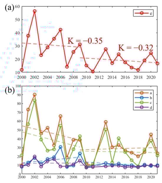
Figure 12.
Annual average TSS concentration change in area a–e ((a) for area e, and (b) for areas a–d. Areas a–d are square areas with an area of 4 km2 on the west side of the upper reaches, east side of the upper reaches, west side of the lower reaches, and east side of the lower reaches of the HZMB. Area e is a rectangular area covering the HZMB).
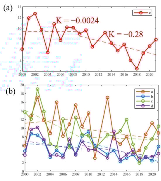
Figure 13.
Annual average Chl-a concentration change in area a–e ((a) for area e, and (b) for areas a–d. Areas a–d are square areas with an area of 4 km2 on the west side of the upper reaches, east side of the upper reaches, west side of the lower reaches, and east side of the lower reaches of the HZMB. Area e is a rectangular area covering the HZMB).
Comparison of areas a–d reveals that the TSS in the waters located on the west side of the HZMB is significantly higher than that on the eastern side because the Pearl River current will be deflected to the west. As the rates of the TSS in areas a and c on both sides of the bridge abutment and the artificial island are greater than 0 while the rates of TSS in areas b and d on both sides of the submarine tunnel are less than 0, we hypothesize that this is due to the water-blocking effect of the bridge abutment and the artificial island, and that this effect is more evident in the upstream area of the river. Moreover, areas b and d are located in the core area of the PRE Chinese White Dolphin National Nature Reserve, and the TSS has always been maintained at a relatively stable and low level due to anthropogenic environmental management measures.
As can be seen from Figure 13b, Chl-a is higher in areas a and c than in areas b and d. This is consistent with 3.1.2 and is mainly due to the west side of the estuary. The rate of Chl-a in areas a, b, and d were all less than 0, whereas the rate of Chl-a in area c was greater than 0. This may be due to the fact that the obstruction of bridges and artificial islands between areas a and c caused the slowing down of the water flow in area c and the increase in the residence time of phytoplankton in area c, which promoted the growth of phytoplankton. In contrast, areas b and d were not obstructed by bridges and artificial islands, so the changes in Chl-a in the two areas were consistent, and the concentrations were close to each other.
4. Discussion
4.1. Comparison of XGBoost-Based Algorithms with the Existing Algorithms
Figure 14b,c compares the estimated and measured concentration of TSS based on Liu et al.’s two algorithms [5], as shown in Equations (A1) and (A2). A comparison between the estimated and measured concentration of Chl-a based on the RTA_17 algorithm [47] (Equation (A3)) and OC2 algorithm [48] (Equation (A4)) appears in Figure 14e,f. All four algorithms used the remotely sensed reflectance obtained from Landsat images as their input; the areas under consideration were either the PRE and its coastal waters or the water around Hong Kong. From the comparisons in Figure 14, it can be observed that, in estimating TSS and Chl-a concentrations, the estimated values’ deviation from the 1:1 line for the four algorithms was larger than that found in the results yielded by the XGBoost-based algorithms; furthermore, the RMSE and MAE were much larger than those associated with the XGBoost-based algorithms. Additionally, the RTA_17_algorithm and OC2 algorithm’s estimations of Chl-a grossly overestimated the proportion of Chl-a at low concentrations and, conversely, grossly underestimated it at high concentrations. In contrast, the XGBoost-based algorithms performed well, in general, despite a relatively small amount of overestimation or underestimation.
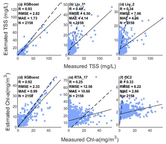
Figure 14.
Comparison of different algorithms estimated and in situ measured TSS and Chl-a for all matched data pairs (a,d) XGBoost-based algorithm, (b,c) Liu et al.’s two algorithms, (e) RTA_17 algorithm, (f) OC2 algorithm.
4.2. Performance of the Algorithm at Different Concentrations
In this study, we divided the matched data set into four concentration intervals according to the in situ data. In situ TSS ranged from 0 to 140 mg/L, whereas in situ Chl-a ranged from 0 to 56 mg/m3. Due to the larger concentration range of TSS in situ, the setting of the first concentration range of the two factors was different (see Table 4). The amount of in situ TSS was similar in 0–2 mg/L, 2–5 mg/L, and 5–10 mg/L concentrations; however, the amount above 10 mg/L was significantly lower than that in other ranges. According to RMSLE and MAPE, the algorithm performed best when TSS was in the range of 5–10 mg/L; in this case, MAPE was 23.97%. Conversely, the algorithm performed poorly when TSS was in the range of 0–2 mg/L. More than half of the total amount of in situ Chl-a data was found in the range of 1–5 mg/m3, whereas 17% of the total amount was in the range of 0–1 mg/m3. In addition, 13% and 10% of the total amount were in the ranges of 5–10 mg/m3 and more than 10 mg/m3, respectively. The algorithm performed better when in situ Chl-a > 10 mg/m3; furthermore, the error increased as the concentration of Chl-a decreased. Both TSS and Chl-a had the largest error in their smallest concentration range, explainable by the more sensitive performance in terms of the error smaller concentrations, which was more likely to lead to a large MAPE.
Table 4.
Performance assessment of XGboost-based algorithm of different TSS (unit: mg/L) and Chl-a (unit: mg/m3) concentration.
5. Conclusions
In this study, we matched 262 Landsat 5 TM images and 185 Landsat 8 OLI images with TSS and Chl-a data measured in situ, thus obtaining 2158 sets of matched data spanning 21 years. The bands used for our calculation were selected from dozens of band combinations with TSS and Chl-a correlation coefficients R. One algorithm used to estimate TSS and Chl-a in the PRE region was constructed based on the XGBoost algorithm, whereas the other featured a single-layer BPNN algorithm in its construction. In a comparison of the two algorithms in terms of R, R2, RMSE, and MAE, the XGBoost algorithm demonstrated better performance and was ultimately selected for our estimation of the spatial and temporal distribution of TSS and Chl-a levels in the PRE region from 2000 to 2021. The results yielded evident spatial and temporal characteristics. In terms of spatial distribution, high TSS and Chl-a appeared near each inlet on the western side of the PRE, and high values of TSS and Chl-a existed in Shenzhen Bay, reflecting human influence. Seasonally, the high values of TSS and Chl-a mostly appeared in spring and summer but were relatively low in fall and winter. TSS and Chl-a were significantly higher in the abundant water period than in the dry water period; in particular, a band of high Chl-a distribution was observed in the area from the south of Moujiamen to the south of Hong Kong, north of Tandang Island, during the abundant water period.
Our analysis of the multi-year changes in TSS and Chl-a in five areas near the HZMB revealed that since the beginning of the construction of the HZMB, the change in the rate of TSS covering the whole bridge and the area on the bridge’s west side was greater than 0. In addition, TSS levels in the area on the west side of the bridge displayed an upward trend, having changed from their original downward trend. Comparing the results for the upstream area on the west side to those for the downstream area revealed a more evident change in the west-side upstream area. The areas on the east side of the bridge on both sides of the submarine tunnel demonstrated a change in the rate of TSS of less than 0; that said, the changes in TSS and TSS in the upstream and downstream areas were very similar. By comparison, the changes in the rate of Chl-a were all less than 0 in the entire bridge coverage area, as well as the upstream area on the west side of the bridge, and the areas on both sides of the submarine tunnel on the east side of the bridge, but, in the downstream area on the east side of the bridge, the change in the rate of Chl-a was greater than 0.
Our study findings have positive implications for environmental management policies. Our plans for future studies include using satellite data with higher temporal resolution, incorporating new field studies, examining more modeling methods, and increasing our understanding of the hydrodynamic situation in conducting further research.
Author Contributions
Conceptualization, J.L. and Y.Z.; methodology, Z.Q.; software, J.Y.T.; validation, J.F., K.P.W. and Z.Q.; formal analysis, J.L. and Z.Q.; investigation, J.L.; resources, J.Y.T.; data curation, J.L. and J.F.; writing—original draft preparation, J.L.; writing—review and editing, Z.Q., Y.W. and Y.Z.; visualization, J.L.; supervision, Y.Z.; project administration, Z.Q.; funding acquisition, Z.Q. All authors have read and agreed to the published version of the manuscript.
Funding
This research was funded by the National Natural Science Foundation (U1901215, 41976165), the Marine Special Program of Jiangsu Province in China (JSZRHYKJ202007), and the Natural Scientific Foundation of Jiangsu Province (BK20181413).
Data Availability Statement
Publicly available datasets were used in this study. These data can be found here: [https://www.usgs.gov/, accessed on 15 January 2023; https://cd.epic.epd.gov.hk/EPICRIVER/marine/, accessed on 18 January 2023].
Acknowledgments
The data from Hong Kong Observatory, AVISO, and NOAA-CPC are highly appreciated.
Conflicts of Interest
The authors declare no conflict of interest.
Appendix A
Equations (A1) and (A2) show two algorithms for the TSS concentrations estimated by Liu et al. [5] Equation (A3) is the RTA_17 algorithm [47] used to estimate Chl-a concentrations, and equation (A4) is the OC2 algorithm [48] used to estimate Chl-a concentrations, respectively.
where in Equation (3).
References
- Harding, L.W.; Mallonee, M.E.; Perry, E.S. Toward a Predictive Understanding of Primary Productivity in a Temperate, Partially Stratified Estuary. Estuar. Coast. Shelf Sci. 2002, 55, 437–463. [Google Scholar] [CrossRef]
- Guo, J.; Ma, C.; Ai, B.; Xu, X.; Huang, W.; Zhao, J. Assessing the Effects of the Hong Kong-Zhuhai-Macau Bridge on the Total Suspended Solids in the Pearl River Estuary Based on Landsat Time Series. J. Geophys. Res. Ocean. 2020, 125, e2020JC016202. [Google Scholar] [CrossRef]
- Barbier, E.B.; Hacker, S.D.; Kennedy, C.; Koch, E.W.; Stier, A.C.; Silliman, B.R. The Value of Estuarine and Coastal Ecosystem Services. Ecol. Monogr. 2011, 81, 169–193. [Google Scholar] [CrossRef]
- Sari, V.; Dos Reis Castro, N.M.; Pedrollo, O.C. Estimate of Suspended Sediment Concentration from Monitored Data of Turbidity and Water Level Using Artificial Neural Networks. Water Resour. Manag. 2017, 31, 4909–4923. [Google Scholar] [CrossRef]
- Liu, F.; Zhang, T.; Ye, H.; Tang, S. Using Satellite Remote Sensing to Study the Effect of Sand Excavation on the Suspended Sediment in the Hong Kong-Zhuhai-Macau Bridge Region. Water 2021, 13, 435. [Google Scholar] [CrossRef]
- Zhang, X.; Huang, J.; Chen, J.; Zhao, Y. Remote Sensing Monitoring of Total Suspended Solids Concentration in Jiaozhou Bay Based on Multi-Source Data. Ecol. Indic. 2023, 154, 110513. [Google Scholar] [CrossRef]
- Harris, C.K. Across-Shelf Sediment Transport: Interactions between Suspended Sediment and Bed Sediment. J. Geophys. Res. 2002, 107, 3008. [Google Scholar] [CrossRef]
- Bilotta, G.S.; Brazier, R.E. Understanding the Influence of Suspended Solids on Water Quality and Aquatic Biota. Water Res. 2008, 42, 2849–2861. [Google Scholar] [CrossRef] [PubMed]
- Dai, Y.; Yang, S.; Zhao, D.; Hu, C.; Xu, W.; Anderson, D.M.; Li, Y.; Song, X.-P.; Boyce, D.G.; Gibson, L.; et al. Coastal Phytoplankton Blooms Expand and Intensify in the 21st Century. Nature 2023, 615, 280–284. [Google Scholar] [CrossRef]
- Paerl, H.W. Assessing and Managing Nutrient-Enhanced Eutrophication in Estuarine and Coastal Waters: Interactive Effects of Human and Climatic Perturbations. Ecol. Eng. 2006, 26, 40–54. [Google Scholar] [CrossRef]
- Deng, T.; Chau, K.-W.; Duan, H.-F. Machine Learning Based Marine Water Quality Prediction for Coastal Hydro-Environment Management. J. Environ. Manag. 2021, 284, 112051. [Google Scholar] [CrossRef]
- Kravitz, J.; Matthews, M.; Bernard, S.; Griffith, D. Application of Sentinel 3 OLCI for Chl-a Retrieval over Small Inland Water Targets: Successes and Challenges. Remote Sens. Environ. 2020, 237, 111562. [Google Scholar] [CrossRef]
- Liu, G.; Li, L.; Song, K.; Li, Y.; Lyu, H.; Wen, Z.; Fang, C.; Bi, S.; Sun, X.; Wang, Z.; et al. An OLCI-Based Algorithm for Semi-Empirically Partitioning Absorption Coefficient and Estimating Chlorophyll a Concentration in Various Turbid Case-2 Waters. Remote Sens. Environ. 2020, 239, 111648. [Google Scholar] [CrossRef]
- Zhao, J.; Zhang, F.; Chen, S.; Wang, C.; Chen, J.; Zhou, H.; Xue, Y. Remote Sensing Evaluation of Total Suspended Solids Dynamic with Markov Model: A Case Study of Inland Reservoir across Administrative Boundary in South China. Sensors 2020, 20, 6911. [Google Scholar] [CrossRef] [PubMed]
- Wang, C.; Li, W.; Chen, S.; Li, D.; Wang, D.; Liu, J. The Spatial and Temporal Variation of Total Suspended Solid Concentration in Pearl River Estuary during 1987–2015 Based on Remote Sensing. Sci. Total Environ. 2018, 618, 1125–1138. [Google Scholar] [CrossRef] [PubMed]
- Kolluru, S.; Tiwari, S.P. Modeling Ocean Surface Chlorophyll-a Concentration from Ocean Color Remote Sensing Reflectance in Global Waters Using Machine Learning. Sci. Total Environ. 2022, 844, 157191. [Google Scholar] [CrossRef]
- Adjovu, G.E.; Stephen, H.; James, D.; Ahmad, S. Measurement of Total Dissolved Solids and Total Suspended Solids in Water Systems: A Review of the Issues, Conventional, and Remote Sensing Techniques. Remote Sens. 2023, 15, 3534. [Google Scholar] [CrossRef]
- Maier, H.R.; Dandy, G.C. Neural Networks for the Prediction and Forecasting of Water Resources Variables: A Review of Modelling Issues and Applications. Environ. Model. Softw. 2000, 15, 101–124. [Google Scholar] [CrossRef]
- McCabe, M.F.; Rodell, M.; Alsdorf, D.E.; Miralles, D.G.; Uijlenhoet, R.; Wagner, W.; Lucieer, A.; Houborg, R.; Verhoest, N.E.C.; Franz, T.E.; et al. The Future of Earth Observation in Hydrology. Hydrol. Earth Syst. Sci. 2017, 21, 3879–3914. [Google Scholar] [CrossRef] [PubMed]
- Sinha, A.; Abernathey, R. Estimating Ocean Surface Currents With Machine Learning. Front. Mar. Sci. 2021, 8, 672477. [Google Scholar] [CrossRef]
- Fan, Y.; Li, W.; Chen, N.; Ahn, J.-H.; Park, Y.-J.; Kratzer, S.; Schroeder, T.; Ishizaka, J.; Chang, R.; Stamnes, K. OC-SMART: A Machine Learning Based Data Analysis Platform for Satellite Ocean Color Sensors. Remote Sens. Environ. 2021, 253, 112236. [Google Scholar] [CrossRef]
- Ma, C.; Zhao, J.; Ai, B.; Sun, S.; Yang, Z. Machine Learning Based Long-Term Water Quality in the Turbid Pearl River Estuary, China. JGR Ocean. 2022, 127, e2021JC018017. [Google Scholar] [CrossRef]
- Wang, Z.; Mao, Z.; Zhang, L.; Zhang, X.; Yuan, D.; Li, Y.; Wu, Z.; Huang, H.; Zhu, Q. Observations of the Impacts of Hong Kong International Airport on Water Quality from 1986 to 2022 Using Landsat Satellite. Remote Sens. 2023, 15, 3146. [Google Scholar] [CrossRef]
- Wang, X.; Gong, Z.; Pu, R. Estimation of Chlorophyll a Content in Inland Turbidity Waters Using WorldView-2 Imagery: A Case Study of the Guanting Reservoir, Beijing, China. Environ. Monit. Assess. 2018, 190, 620. [Google Scholar] [CrossRef]
- Gómez, D.; Salvador, P.; Sanz, J.; Casanova, J.L. A New Approach to Monitor Water Quality in the Menor Sea (Spain) Using Satellite Data and Machine Learning Methods. Environ. Pollut. 2021, 286, 117489. [Google Scholar] [CrossRef]
- Pahlevan, N.; Smith, B.; Alikas, K.; Anstee, J.; Barbosa, C.; Binding, C.; Bresciani, M.; Cremella, B.; Giardino, C.; Gurlin, D.; et al. Simultaneous Retrieval of Selected Optical Water Quality Indicators from Landsat-8, Sentinel-2, and Sentinel-3. Remote Sens. Environ. 2022, 270, 112860. [Google Scholar] [CrossRef]
- Du, C.; Wang, Q.; Li, Y.; Lyu, H.; Zhu, L.; Zheng, Z.; Wen, S.; Liu, G.; Guo, Y. Estimation of Total Phosphorus Concentration Using a Water Classification Method in Inland Water. Int. J. Appl. Earth Obs. Geoinf. 2018, 71, 29–42. [Google Scholar] [CrossRef]
- Sagawa, T.; Yamashita, Y.; Okumura, T.; Yamanokuchi, T. Satellite Derived Bathymetry Using Machine Learning and Multi-Temporal Satellite Images. Remote Sens. 2019, 11, 1155. [Google Scholar] [CrossRef]
- Tiyasha, T.; Tung, T.M.; Bhagat, S.K.; Tan, M.L.; Jawad, A.H.; Mohtar, W.H.M.W.; Yaseen, Z.M. Functionalization of Remote Sensing and On-Site Data for Simulating Surface Water Dissolved Oxygen: Development of Hybrid Tree-Based Artificial Intelligence Models. Mar. Pollut. Bull. 2021, 170, 112639. [Google Scholar] [CrossRef] [PubMed]
- Liu, B.; Peng, S.; Liao, Y.; Long, W. The causes and impacts of water resources crises in the Pearl River Delta. J. Clean. Prod. 2018, 177, 413–425. [Google Scholar] [CrossRef]
- Qian, W.; Zhang, S.; Tong, C.; Sardans, J.; Peñuelas, J.; Li, X. Long-Term Patterns of Dissolved Oxygen Dynamics in the Pearl River Estuary. JGR Biogeosci. 2022, 127, e2022JG006967. [Google Scholar] [CrossRef]
- Zhang, J.; Yu, Z.G.; Wang, J.T.; Ren, J.L.; Chen, H.T.; Xiong, H.; Dong, L.X.; Xu, W.Y. The Subtropical Zhujiang (Pearl River) Estuary: Nutrient, Trace Species and Their Relationship to Photosynthesis. Estuar. Coast. Shelf Sci. 1999, 49, 385–400. [Google Scholar] [CrossRef]
- Yang, Y.; Cheng, Q.; Tsou, J.-Y.; Wong, K.-P.; Men, Y.; Zhang, Y. Multiscale Analysis and Prediction of Sea Level in the Northern South China Sea Based on Tide Gauge and Satellite Data. J. Mar. Sci. Eng. 2023, 11, 1203. [Google Scholar] [CrossRef]
- Duan, W.; Congress, S.S.C.; Cai, G.; Puppala, A.J.; Dong, X.; Du, Y. Empirical Correlations of Soil Parameters Based on Piezocone Penetration Tests (CPTU) for Hong Kong-Zhuhai-Macau Bridge (HZMB) Project. Transp. Geotech. 2021, 30, 100605. [Google Scholar] [CrossRef]
- Xie, Q.; Gui, D.; Liu, W.; Wu, Y. Risk for Indo-Pacific Humpback Dolphins (Sousa chinensis) and Human Health Related to the Heavy Metal Levels in Fish from the Pearl River Estuary, China. Chemosphere 2020, 240, 124844. [Google Scholar] [CrossRef]
- Hafeez, S.; Wong, M.; Ho, H.; Nazeer, M.; Nichol, J.; Abbas, S.; Tang, D.; Lee, K.; Pun, L. Comparison of Machine Learning Algorithms for Retrieval of Water Quality Indicators in Case-II Waters: A Case Study of Hong Kong. Remote Sens. 2019, 11, 617. [Google Scholar] [CrossRef]
- Maciel, F.P.; Pedocchi, F. Evaluation of ACOLITE Atmospheric Correction Methods for Landsat-8 and Sentinel-2 in the Río de La Plata Turbid Coastal Waters. Int. J. Remote Sens. 2022, 43, 215–240. [Google Scholar] [CrossRef]
- Zhu, X.; Guo, H.; Huang, J.J.; Tian, S.; Xu, W.; Mai, Y. An Ensemble Machine Learning Model for Water Quality Estimation in Coastal Area Based on Remote Sensing Imagery. J. Environ. Manag. 2022, 323, 116187. [Google Scholar] [CrossRef]
- Chen, T.; Guestrin, C. XGBoost: A Scalable Tree Boosting System. In Proceedings of the 22nd ACM SIGKDD International Conference on Knowledge Discovery and Data Mining, San Francisco, CA, USA, 13–17 August 2016; pp. 785–794. [Google Scholar]
- Lei, S.; Luo, J.; Tao, X.; Qiu, Z. Remote Sensing Detecting of Yellow Leaf Disease of Arecanut Based on UAV Multisource Sensors. Remote Sens. 2021, 13, 4562. [Google Scholar] [CrossRef]
- Choo, J.; Cherukuru, N.; Lehmann, E.; Paget, M.; Mujahid, A.; Martin, P.; Müller, M. Spatial and Temporal Dynamics of Suspended Sediment Concentrations in Coastal Waters of South China Sea, off Sarawak, Borneo: Ocean Colour Remote Sensing Observations and Analysis. Biogeosciences 2022, 19, 5837–5857. [Google Scholar] [CrossRef]
- Zhang, G.; Cheng, W.; Chen, L.; Zhang, H.; Gong, W. Transport of Riverine Sediment from Different Outlets in the Pearl River Estuary during the Wet Season. Mar. Geol. 2019, 415, 105957. [Google Scholar] [CrossRef]
- Cao, B.; Qiu, J.; Zhang, W.; Xie, X.; Lu, X.; Yang, X.; Li, H. Retrieval of Suspended Sediment Concentrations in the Pearl River Estuary Using Multi-Source Satellite Imagery. Remote Sens. 2022, 14, 3896. [Google Scholar] [CrossRef]
- Li, L.; Lu, S.; Jiang, T.; Li, X. Seasonal Variation of Size-Fractionated Phytoplankton in the Pearl River Estuary. Chin. Sci. Bull. 2013, 58, 2303–2314. [Google Scholar] [CrossRef]
- Nukapothula, S.; Chen, C.; Wu, J. Long-Term Distribution Patterns of Remotely Sensed Water Quality Variables in Pearl River Delta, China. Estuar. Coast. Shelf Sci. 2019, 221, 90–103. [Google Scholar] [CrossRef]
- Zhan, W.; Wu, J.; Wei, X.; Tang, S.; Zhan, H. Spatio-Temporal Variation of the Suspended Sediment Concentration in the Pearl River Estuary Observed by MODIS during 2003–2015. Cont. Shelf Res. 2019, 172, 22–32. [Google Scholar] [CrossRef]
- Nazeer, M.; Bilal, M.; Alsahli, M.; Shahzad, M.; Waqas, A. Evaluation of Empirical and Machine Learning Algorithms for Estimation of Coastal Water Quality Parameters. ISPRS Int. J. Geo-Inf. 2017, 6, 360. [Google Scholar] [CrossRef]
- Franz, B.A.; Bailey, S.W.; Kuring, N.; Werdell, P.J. Ocean Color Measurements with the Operational Land Imager on Landsat-8: Implementation and Evaluation in SeaDAS. J. Appl. Remote Sens. 2015, 9, 096070. [Google Scholar] [CrossRef]


Disclaimer/Publisher’s Note: The statements, opinions and data contained in all publications are solely those of the individual author(s) and contributor(s) and not of MDPI and/or the editor(s). MDPI and/or the editor(s) disclaim responsibility for any injury to people or property resulting from any ideas, methods, instructions or products referred to in the content. |
© 2023 by the authors. Licensee MDPI, Basel, Switzerland. This article is an open access article distributed under the terms and conditions of the Creative Commons Attribution (CC BY) license (https://creativecommons.org/licenses/by/4.0/).