
Hyperspectral Image Classification Promotion Using Dynamic Convolution Based on Structural Re-Parameterization

 , and
, and
Abstract
:
1. Introduction
2. Materials and Methods
2.1. Data Preprocessing
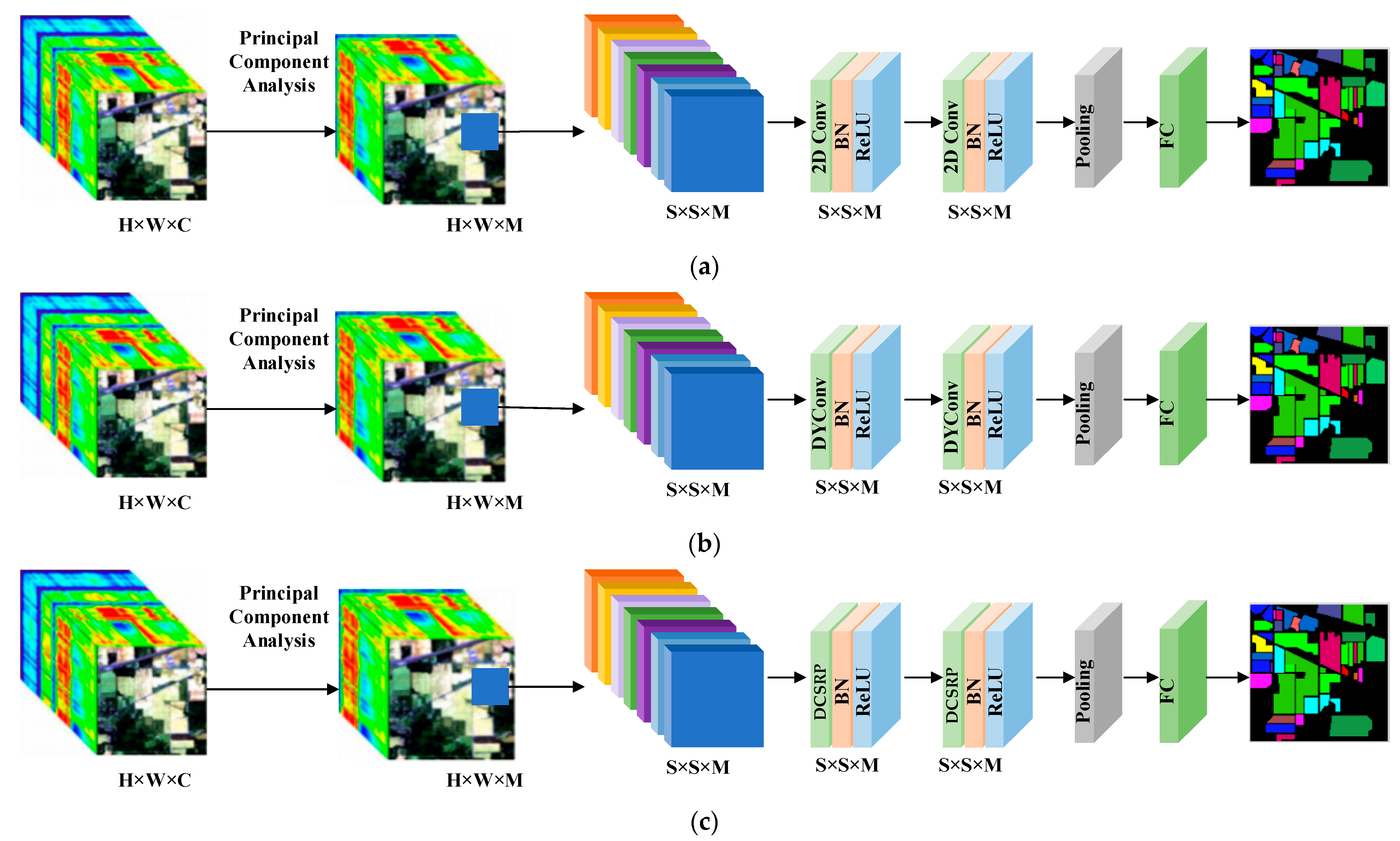
2.2. Overall Framework of Proposed Method
2.3. Dynamic Convolution
2.4. Structural Re-Parameterization
3. Experiments
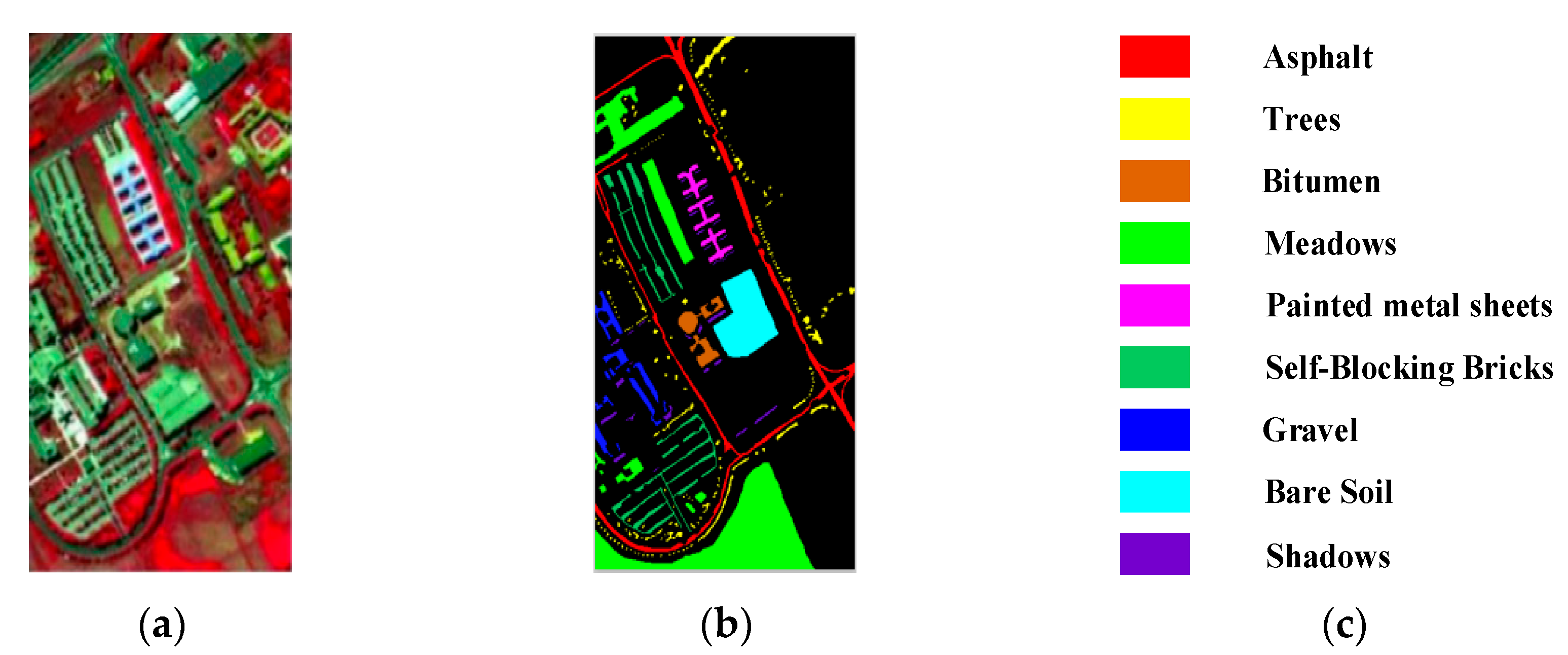
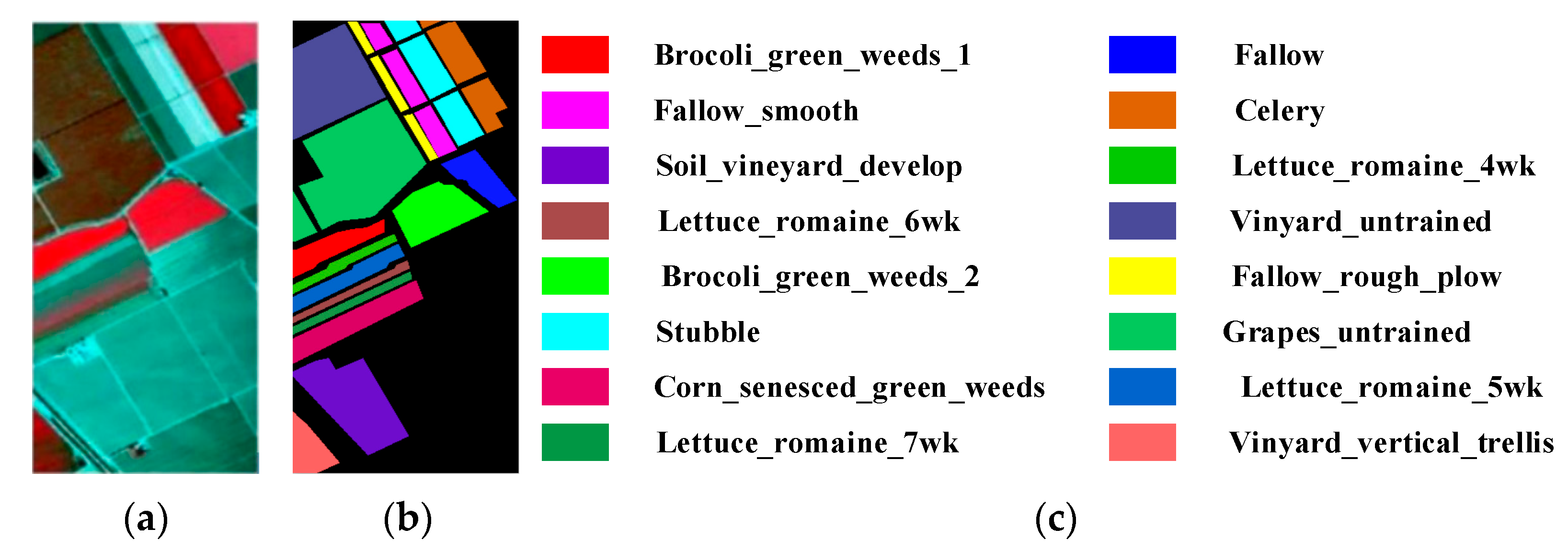
3.1. Data Description
3.1.1. Indian Pines
3.1.2. University of Pavia
3.1.3. Salinas
3.2. Experimental Configuration
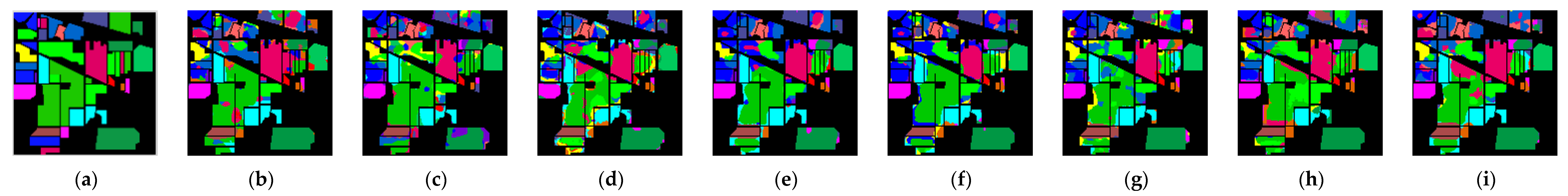
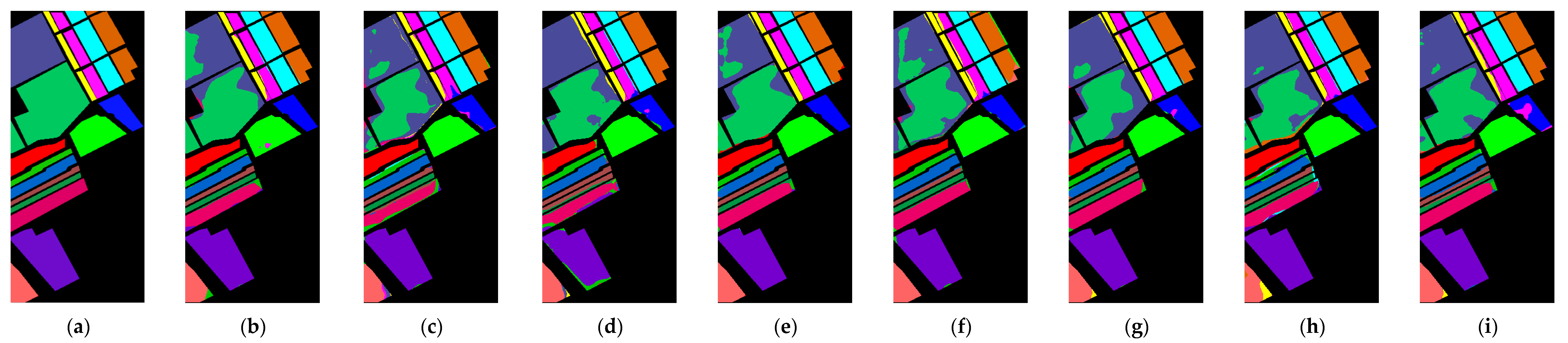
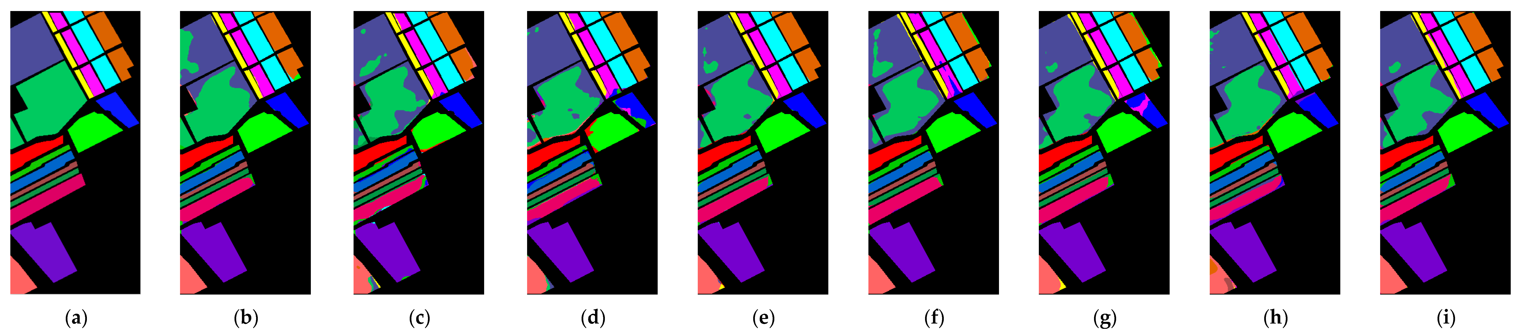
3.3. Experimental Results
3.3.1. Ablation Studies
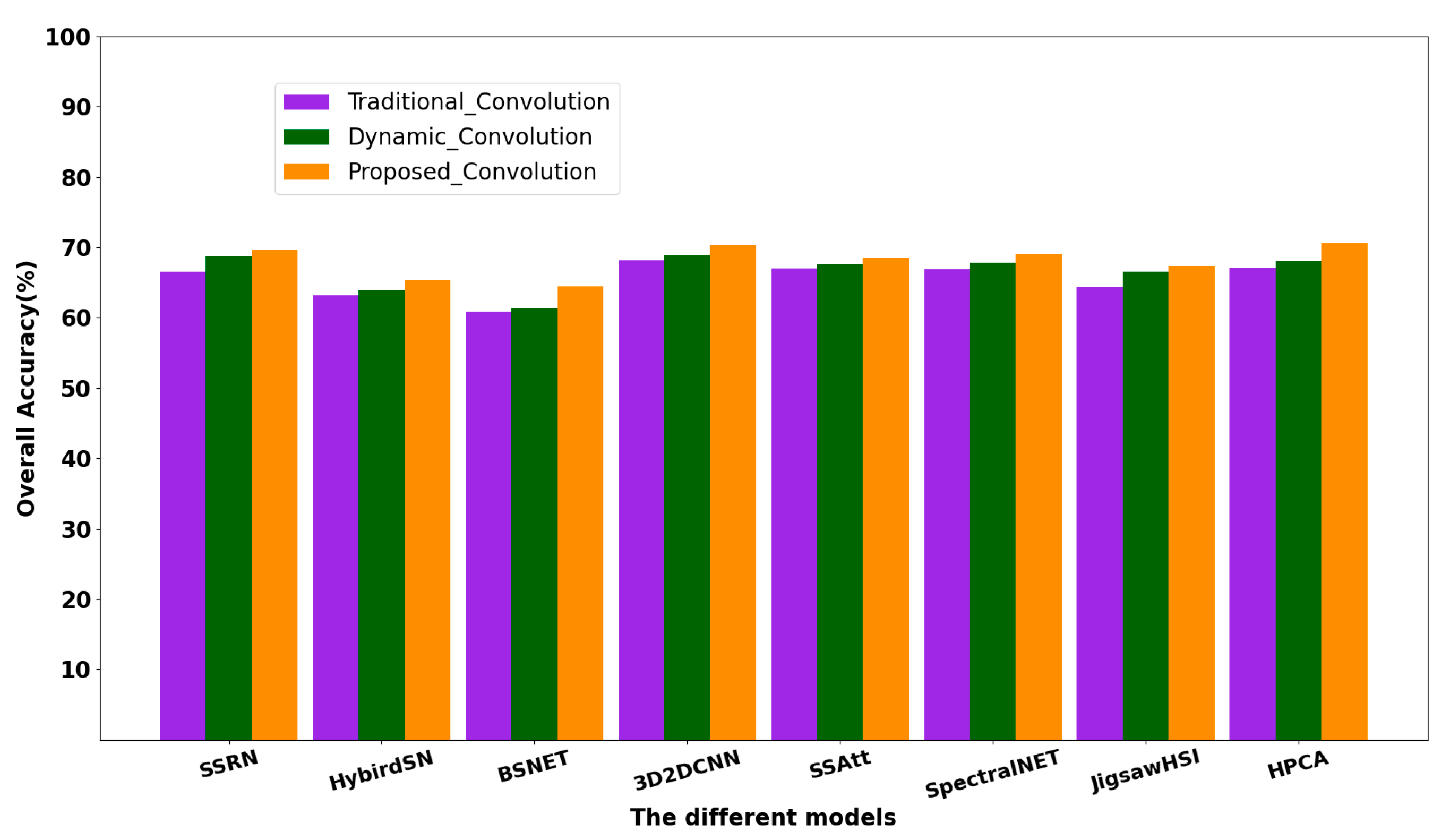
3.3.2. Compared Results in Different Methods
3.3.3. Experimental Results of Different Sizes of Convolutional Kernels
4. Discussion
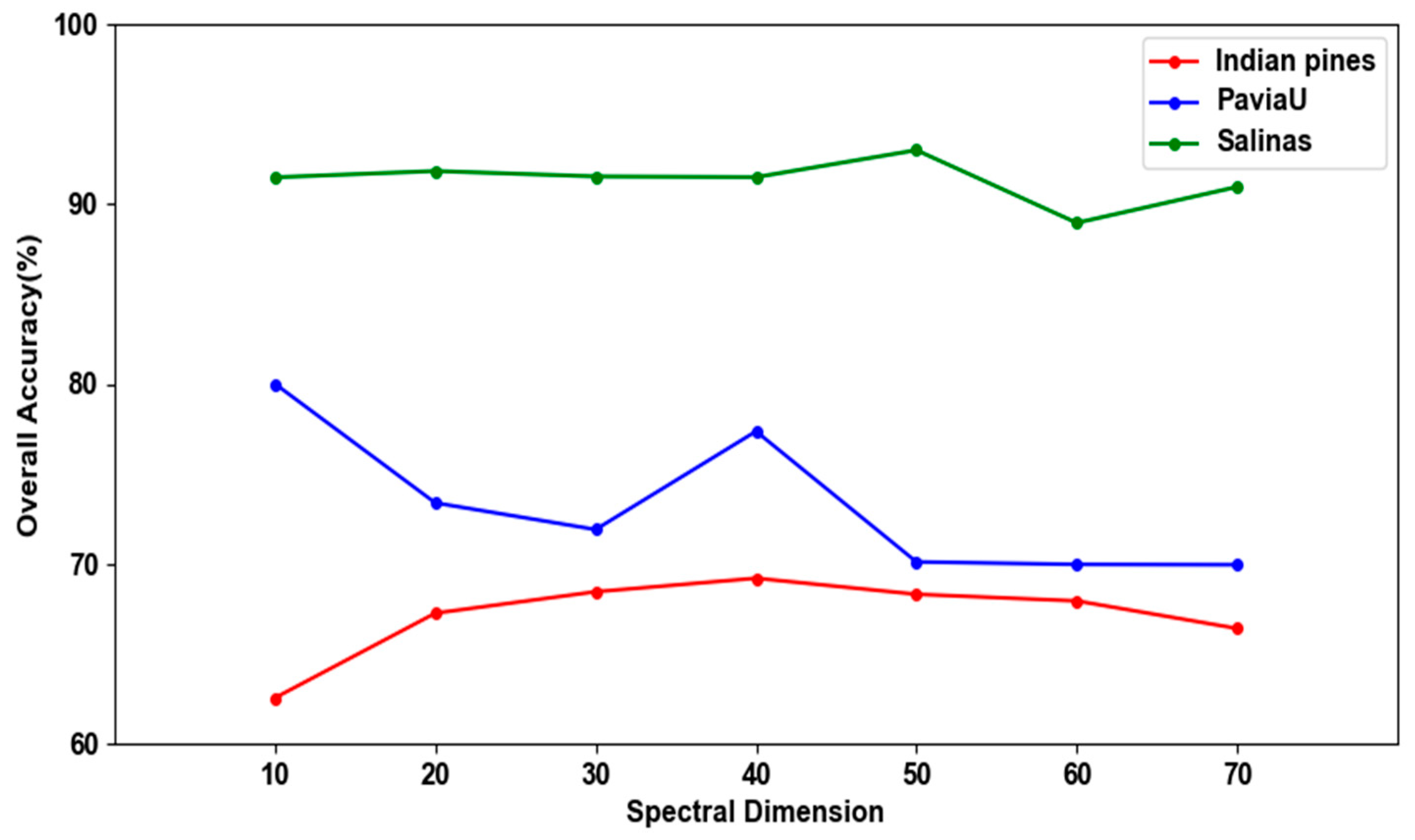
4.1. The Influence of the Number of Parallel Re-Parameterization Kernels on Experimental Results
4.2. The Influence of Different Channel and Spatial Sizes on Experimental Results
4.3. The Influence of Different Re-Parameterization Kernel Sizes
5. Conclusions
Author Contributions
Funding
Data Availability Statement
Conflicts of Interest
References
- Flores, H.; Lorenz, S.; Jackisch, R.; Tusa, L.; Contreras, I.C.; Zimmermann, R.; Gloaguen, R. UAS-based hyperspectral environmental monitoring of acid mine drainage affected waters. Minerals 2021, 11, 182. [Google Scholar] [CrossRef]
- Gao, A.F.; Rasmussen, B.; Kulits, P.; Scheller, E.L.; Greenberger, R.; Ehlmann, B.L. Generalized unsupervised clustering of hyperspectral images of geological targets in the near infrared. In Proceedings of the IEEE/CVF Conference on Computer Vision and Pattern Recognition, Nashville, TN, USA, 19–25 June 2021; pp. 4294–4303. [Google Scholar]
- Zhou, S.; Sun, L.; Ji, Y. Germination Prediction of Sugar Beet Seeds Based on HSI and SVM-RBF. In Proceedings of the 4th International Conference on Measurement, Information and Control (ICMIC), Harbin, China, 23–25 August 2019; pp. 93–97. [Google Scholar]
- Haq, M.A.; Rahaman, G.; Baral, P.; Ghosh, A. Deep learning based supervised image classification using UAV images for forest areas classification. J. Indian Soc. Remote Sens. 2021, 49, 601–606. [Google Scholar] [CrossRef]
- Pan, B.; Shi, Z.; An, Z.; Jiang, Z.; Ma, Y. A novel spectral-unmixing-based green algae area estimation method for GOCI data. IEEE J. Sel. Top. Appl. Earth Obs. Remote Sens. 2016, 10, 437–449. [Google Scholar] [CrossRef]
- Makki, I.; Younes, R.; Francis, C.; Bianchi, T.; Zucchetti, M. A survey of landmine detection using hyperspectral imaging. ISPRS J. Photogramm. Remote Sens. 2017, 124, 40–53. [Google Scholar] [CrossRef]
- Shimoni, M.; Haelterman, R.; Perneel, C. Hypersectral imaging for military and security applications: Combining myriad processing and sensing techniques. IEEE Geosci. Remote Sens. Mag. 2019, 7, 101–117. [Google Scholar] [CrossRef]
- Nigam, R.; Bhattacharya, B.K.; Kot, R.; Chattopadhyay, C. Wheat blast detection and assessment combining ground-based hyperspectral and satellite based multispectral data. Int. Arch. Photogramm. Remote Sens. Spat. Inf. Sci. 2019, 42, 473–475. [Google Scholar] [CrossRef]
- Gualtieri, J.A.; Cromp, R.F. Support Vector Machines for Hyperspectral Remote Sensing Classification. In Proceedings of the 27th AIPR Workshop: Advances in Computer-Assisted Recognition, Washington, DC, USA, 14–16 October 1998; SPIE: Bellingham, WA, USA, 1999; Volume 3584, pp. 221–232. [Google Scholar]
- Jain, V.; Phophalia, A. Exponential Weighted Random Forest for Hyperspectral Image Classification. In Proceedings of the IGARSS 2019—2019 IEEE International Geoscience and Remote Sensing Symposium, Yokohama, Japan, 28 July–2 August 2019; pp. 3297–3300. [Google Scholar]
- Chen, Y.; Lin, Z.; Zhao, X. Riemannian manifold learning based k-nearest-neighbor for hyperspectral image classification. In Proceedings of the 2013 IEEE International Geoscience and Remote Sensing Symposium-IGARSS, Melbourne, Australia, 21–26 July 2013; pp. 1975–1978. [Google Scholar]
- Wu, Z.; Shi, L.; Li, J.; Wang, Q.; Sun, L.; Wei, Z.; Plaza, J.; Plaza, A. GPU parallel implementation of spatially adaptive hyperspectral image classification. IEEE J. Sel. Top. Appl. Earth Obs. Remote Sens. 2017, 11, 1131–1143. [Google Scholar] [CrossRef]
- Chen, Y.; Nasrabadi, N.M.; Tran, T.D. Hyperspectral image classification using dictionary-based sparse representation. IEEE Trans. Geosci. Remote Sens. 2011, 49, 3973–3985. [Google Scholar] [CrossRef]
- Cheng, G.; Li, Z.; Han, J.; Yao, X.; Guo, L. Exploring hierarchical convolutional features for hyperspectral image classification. IEEE Trans. Geosci. Remote Sens. 2018, 56, 6712–6722. [Google Scholar] [CrossRef]
- Li, J.; Marpu, P.R.; Plaza, A.; Bioucas-Dias, J.M.; Benediktsson, J.A. Generalized composite kernel framework for hyperspectral image classification. IEEE Trans. Geosci. Remote Sens. 2013, 51, 4816–4829. [Google Scholar] [CrossRef]
- Zhou, Y.; Peng, J.; Chen, C.L.P. Extreme learning machine with composite kernels for hyperspectral image classification. IEEE J. Sel. Top. Appl. Earth Obs. Remote Sens. 2014, 8, 2351–2360. [Google Scholar] [CrossRef]
- Fan, W.; Zhang, R.; Wu, Q. Hyperspectral image classification based on PCA network. In Proceedings of the 2016 8th Workshop on Hyperspectral Image and Signal Processing: Evolution in Remote Sensing (WHISPERS), Los Angeles, CA, USA, 21–24 August 2016. [Google Scholar]
- Gao, F.; Dong, J.; Li, B.; Xu, Q. Automatic change detection in synthetic aperture radar images based on PCANet. IEEE Geosci. Remote Sens. Lett. 2016, 13, 1792–1796. [Google Scholar] [CrossRef]
- Zhou, S.; Xue, Z.; Du, P. Semisupervised stacked autoencoder with cotraining for hyperspectral image classification. IEEE Trans. Geosci. Remote Sens. 2019, 57, 3813–3826. [Google Scholar] [CrossRef]
- Shi, C.; Pun, C.M. Multiscale superpixel-based hyperspectral image classification using recurrent neural networks with stacked autoencoders. IEEE Trans. Multimed. 2019, 22, 487–501. [Google Scholar] [CrossRef]
- Midhun, M.E.; Nair, S.R.; Prabhakar, V.T.N.; Kumar, S.S. Deep Model for Classification of Hyperspectral Image Using Restricted Boltzmann Machine. In Proceedings of the International Conference on Interdisciplinary Advances in Applied Computing, Amritapuri, India, 10–11 October 2014; pp. 1–7. [Google Scholar]
- Li, T.; Zhang, J.; Zhang, Y. Classification of Hyperspectral Image Based on Deep Belief Networks. In Proceedings of the 2014 IEEE International Conference on Image Processing (ICIP), Paris, France, 27–30 October 2014; pp. 5132–5136. [Google Scholar]
- Jiang, Z.; Pan, W.D.; Shen, H. Universal Golomb–Rice Coding Parameter Estimation Using Deep Belief Networks for Hyperspectral Image Compression. IEEE J. Sel. Top. Appl. Earth Obs. Remote Sens. 2018, 11, 3830–3840. [Google Scholar] [CrossRef]
- Chen, Y.; Jiang, H.; Li, C.; Jia, X.; Ghamisi, P. Deep feature extraction and classification of hyperspectral images based on convolutional neural networks. IEEE Trans. Geosci. Remote Sens. 2016, 54, 6232–6251. [Google Scholar] [CrossRef]
- Yang, J.; Xiao, L.; Zhao, Y.Q.; Chan, J.C.W. Variational regularization network with attentive deep prior for hyperspectral–multispectral image fusion. IEEE Trans. Geosci. Remote Sens. 2021, 60, 1–17. [Google Scholar] [CrossRef]
- Paoletti, M.E.; Haut, J.M.; Fernandez-Beltran, R.; Plaza, J.; Plaza, A.J.; Pla, F. Deep pyramidal residual networks for spectral–spatial hyperspectral image classification. IEEE Trans. Geosci. Remote Sens. 2018, 57, 740–754. [Google Scholar] [CrossRef]
- Paoletti, M.E.; Haut, J.M.; Fernandez-Beltran, R.; Plaza, J.; Plaza, A.; Li, J.; Pla, F. Capsule networks for hyperspectral image classification. IEEE Trans. Geosci. Remote Sens. 2018, 57, 2145–2160. [Google Scholar] [CrossRef]
- Li, X.; Ding, M.; Gu, Y.; Pižurica, A. An End-to-End Framework for Joint Denoising and Classification of Hyperspectral Images. IEEE Trans. Neural Netw. Learn. Syst. 2023, 34, 3269–3283. [Google Scholar] [CrossRef]
- Xue, J.; Zhao, Y.; Huang, S.; Liao, W.; Chan, J.; Kong, S. Multilayer sparsity-based tensor decomposition for low-rank tensor completion. IEEE Trans. Neural Netw. Learn. Syst. 2021, 33, 6916–6930. [Google Scholar] [CrossRef] [PubMed]
- Zilong, Z.; Li, J.; Luo, Z.; Chapman, M. Spectral–spatial residual network for hyperspectral image classification: A 3-D deep learning framework. IEEE Trans. Geosci. Remote Sens. 2017, 56, 847–858. [Google Scholar]
- Kumar, R.S.; Krishna, G.; Dubey, S.R.; Chaudhuri, B.B. HybridSN: Exploring 3-D-2-D CNN feature hierarchy for hyperspectral image classification. IEEE Geosci. Remote Sens. Lett. 2019, 17, 277–281. [Google Scholar]
- Li, X.; Ding, M.; Pizurca, A. Deep feature fusion via two-stream convolutional neural network for hyperspectral image classification. IEEE Trans. Geosci. Remote Sens. 2020, 58, 2615–2629. [Google Scholar] [CrossRef]
- Ding, C.; Chen, Y.; Li, R.; Wen, D.; Xie, X.; Zhang, L.; Wei, W.; Zhang, Y. Integrating hybrid pyramid feature fusion and coordinate attention for effective small sample hyperspectral image classification. Remote Sens. 2022, 14, 2355. [Google Scholar] [CrossRef]
- Yu, C.; Han, R.; Song, M.; Liu, C.; Chang, C.-I. Feedback attentionbased dense CNN for hyperspectral image classification. IEEE Trans. Geosci. Remote Sens. 2022, 60, 5501916. [Google Scholar]
- Luo, W.; Li, Y.; Urtasun, R.; Zemel, R. Understanding the effective receptive field in deep convolutional neural networks. Adv. Neural Inf. Process. Syst. 2016, 29, 2476. [Google Scholar]
- Krizhevsky, A.; Sutskever, I.; Hinton, G.E. Imagenet classification with deep convolutional neural networks. Adv. Neural Inf. Process. Syst. 2012, 25. [Google Scholar] [CrossRef]
- Szegedy, C.; Ioffe, S.; Vanhoucke, V.; Alemi, A. Inception-v4, Inception-ResNet and the Impact of Residual Connections on Learning. In Proceedings of the AAAI Conference on Artificial Intelligence, San Francisco, CA, USA, 4–9 February 2017; Volume 31. [Google Scholar]
- Szegedy, C.; Liu, W.; Jia, Y.; Sermanet, P.; Reed, S.; Anguelov, D.; Erhan, D.; Vanhoucke, V.; Rabinovich, A. Going Deeper with Convolutions. In Proceedings of the IEEE Conference on Computer Vision and Pattern Recognition, Boston, MA, USA, 7–12 June 2015; pp. 1–9. [Google Scholar]
- Szegedy, C.; Vanhoucke, V.; Ioffe, S.; Shlens, J.; Wojna, Z. Rethinking the Inception Architecture for Computer Vision. In Proceedings of the IEEE Conference on Computer Vision and Pattern Recognition, Las Vegas, NV, USA, 27–30 June 2016; pp. 2818–2826. [Google Scholar]
- Guo, Z.; Zhang, X.; Mu, H.; Heng, W.; Liu, Z.; Wei, Y.; Sun, J. Single path one-shot neural architecture search with uniform sampling. In Proceedings of the Computer Vision–ECCV 2020: 16th European Conference, Glasgow, UK, 23–28 August 2020; pp. 544–560. [Google Scholar]
- Howard, A.; Sandler, M.; Chu, G.; Chen, L.C.; Chen, B.; Tan, M.; Wang, W.; Zhu, Y.; Pang, R.; Vasudevan, V.; et al. Searching for Mobilenetv3. In Proceedings of the IEEE/CVF International Conference on Computer Vision, Seoul, Republic of Korea, 27 October–2 November 2019; pp. 1314–1324. [Google Scholar]
- Liu, H.; Simonyan, K.; Yang, Y. Darts: Differentiable architecture search. arXiv 2018, arXiv:1806.09055. [Google Scholar]
- Barret, Z.; Le Quoc, V. Neural architecture search with reinforcement learning. arXiv 2016, arXiv:1611.01578. [Google Scholar]
- Liu, Z.; Mao, H.; Wu, C.Y.; Feichtenhofer, C.; Darrell, T.; Xie, S. A ConvNet for the 2020s. In Proceedings of the IEEE/CVF Conference on Computer Vision and Pattern Recognition, New Orleans, LA, USA, 18–24 June 2022; pp. 11976–11986. [Google Scholar]
- Shang, R.; Chang, H.; Zhang, W.; Feng, J.; Li, Y. Hyperspectral image classification based on multiscale cross-branch response and second-order channel attention. IEEE Trans. Geosci. Remote Sens. 2022, 60, 5532016. [Google Scholar] [CrossRef]
- Ma, Y.; Liu, Z.; Chen, C.L.P. Multiscale random convolution broad learning system for hyperspectral image classification. IEEE Geosci. Remote Sens. Lett. 2021, 19, 5503605. [Google Scholar] [CrossRef]
- Jayasree, S.; Khanna, Y.; Mukhopadhyay, J. A CNN with Multiscale Convolution for Hyperspectral Image Classification Using Target-Pixel-Orientation Scheme. In Proceedings of the 2021 IEEE International Geoscience and Remote Sensing Symposium IGARSS, Brussels, Belgium, 11–16 July 2021. [Google Scholar]
- Moraga, J.; Duzgun, H.S. JigsawHSI: A network for hyperspectral image classification. arXiv 2022, arXiv:2206.02327. [Google Scholar]
- Ding, X.; Zhang, X.; Han, J.; Ding, G. Scaling up Your Kernels to 31 × 31: Revisiting Large Kernel Design in CNNs. In Proceedings of the IEEE/CVF Conference on Computer Vision and Pattern Recognition, New Orleans, LA, USA, 18–24 June 2022; pp. 11963–11975. [Google Scholar]
- Radosavovic, I.; Kosaraju, R.P.; Girshick, R.; He, K.; Dollár, P. Designing Network Design Spaces. In Proceedings of the IEEE/CVF Conference on Computer Vision and Pattern Recognition, Seattle, WA, USA, 13–19 June 2020; pp. 10428–10436. [Google Scholar]
- Zhang, X.; Zhou, X.; Lin, M.; Sun, J. Shufflenet: An extremely Efficient Convolutional Neural Network for Mobile Devices. In Proceedings of the IEEE Conference on Computer Vision and Pattern Recognition, Salt Lake City, UT, USA, 18–23 June 2018; pp. 6848–6856. [Google Scholar]
- Huang, G.; Liu, Z.; Van Der Maaten, L.; Weinberger, K.Q. Densely Connected Convolutional Networks. In Proceedings of the IEEE Conference on Computer Vision and Pattern Recognition, Honolulu, HI, USA, 21–26 July 2017; pp. 4700–4708. [Google Scholar]
- Simonyan, K.; Zisserman, A. Very deep convolutional networks for large-scale image recognition. arXiv 2014, arXiv:1409.1556. [Google Scholar]
- Cai, Y.; Liu, X.; Cai, Z. BS-Nets: An end-to-end framework for band selection of hyperspectral image. IEEE Trans. Geosci. Remote Sens. 2019, 58, 1969–1984. [Google Scholar] [CrossRef]
- Ge, Z.; Cao, G.; Li, X.; Fu, P. Hyperspectral image classification method based on 2D–3D CNN and multibranch feature fusion. IEEE J. Sel. Top. Appl. Earth Obs. Remote Sens. 2020, 13, 5776–5788. [Google Scholar] [CrossRef]
- Hang, R.; Li, Z.; Liu, Q.; Ghamisi, P.; Bhattacharyya, S.S. Hyperspectral image classification with attention-aided CNNs. IEEE Trans. Geosci. Remote Sens. 2020, 59, 2281–2293. [Google Scholar] [CrossRef]
- Chakraborty, T.; Trehan, U. Spectralnet: Exploring spatial-spectral waveletcnn for hyperspectral image classification. arXiv 2021, arXiv:2104.00341. [Google Scholar]


| Class | Name | Total Samples | Train Samples | Test Samples |
|---|---|---|---|---|
| 1 | Alfalfa | 46 | 5 | 41 |
| 2 | Corn-notill | 1428 | 5 | 1423 |
| 3 | Corn-mintill | 830 | 5 | 825 |
| 4 | Corn | 237 | 5 | 232 |
| 5 | Grass-pasture | 483 | 5 | 478 |
| 6 | Grasstrees | 730 | 5 | 725 |
| 7 | Grass-pasture-mowed | 28 | 5 | 23 |
| 8 | Background | 478 | 5 | 473 |
| 9 | Oats | 20 | 5 | 15 |
| 10 | Soybean-no till | 972 | 5 | 967 |
| 11 | Soybean-min till | 2455 | 5 | 2450 |
| 12 | Soybean-clean | 593 | 5 | 588 |
| 13 | Wheat | 205 | 5 | 200 |
| 14 | Woods | 1265 | 5 | 1260 |
| 15 | Buildings-grass-trees-drives | 386 | 5 | 381 |
| 16 | Stone-steel-towers | 93 | 5 | 88 |
| Total | 10,249 | 80 | 10,169 |
| Class | Name | Total Samples | Train Samples | Test Samples |
|---|---|---|---|---|
| 1 | Asphalt | 6631 | 5 | 6626 |
| 2 | Meadows | 18,649 | 5 | 18,644 |
| 3 | Gravel | 2099 | 5 | 2094 |
| 4 | Trees | 3064 | 5 | 3059 |
| 5 | Painted metal sheets | 1345 | 5 | 1340 |
| 6 | Bare soil | 5029 | 5 | 5024 |
| 7 | Bitumen | 1330 | 5 | 1325 |
| 8 | Self-blocking bricks | 3682 | 5 | 3677 |
| 9 | Shadows | 947 | 5 | 942 |
| Total | 42,776 | 45 | 42,731 |
| Class | Name | Total Samples | Train Samples | Test Samples |
|---|---|---|---|---|
| 1 | Brocoli_green_weeds_1 | 2009 | 5 | 2004 |
| 2 | Brocoli_green_weeds_2 | 3726 | 5 | 3721 |
| 3 | Fallow | 1976 | 5 | 1971 |
| 4 | Fallow rough plow | 1394 | 5 | 1389 |
| 5 | Fallow smooth | 2678 | 5 | 2673 |
| 6 | Stubble | 3959 | 5 | 3954 |
| 7 | Celery | 3579 | 5 | 3574 |
| 8 | Grapes untrained | 11,271 | 5 | 11,266 |
| 9 | Soil vineyard develop | 6203 | 5 | 6198 |
| 10 | Corn senesced green weeds | 3278 | 5 | 3273 |
| 11 | Lettuce_romaine_4wkl | 1068 | 5 | 1063 |
| 12 | Lettuce_romaine_5wkl | 1927 | 5 | 1922 |
| 13 | Lettuce_romaine_6wkl | 916 | 5 | 911 |
| 14 | Lettuce_romaine_7wkl | 1070 | 5 | 1065 |
| 15 | Vineyard untrained | 7268 | 5 | 7263 |
| 16 | Vineyard vertical trellis | 1807 | 5 | 1802 |
| Total | 54,129 | 80 | 54,049 |
| Method | IP | PU | SA | |||
|---|---|---|---|---|---|---|
| OA (%) | AA (%) | OA (%) | AA (%) | OA (%) | AA (%) | |
| Traditional convolution | 62.70 | 76.69 | 70.52 | 74.20 | 90.02 | 92.69 |
| Dynamic convolution | 65.40 | 78.36 | 72.86 | 75.90 | 91.48 | 94.55 |
| Proposed method | 67.25 | 80.03 | 73.38 | 76.45 | 91.83 | 94.60 |
| Different Models | Different Methods | Datasets | ||
|---|---|---|---|---|
| IP | PU | SA | ||
| SSRN [47] | Traditional convolution | 66.50 | 70.97 | 91.05 |
| Dynamic convolution | 68.74 | 73.36 | 91.48 | |
| Proposed method | 69.61 | 75.55 | 91.98 | |
| HybridSN [48] | Traditional convolution | 63.12 | 66.92 | 86.70 |
| Dynamic convolution | 63.87 | 67.61 | 87.57 | |
| Proposed method | 65.32 | 69.06 | 88.25 | |
| BSNET [50] | Traditional convolution | 60.84 | 67.69 | 88.75 |
| Dynamic convolution | 61.36 | 68.70 | 89.04 | |
| Proposed method | 64.47 | 69.05 | 90.41 | |
| 3D2D-CNN [46] | Traditional convolution | 68.12 | 69.09 | 93.16 |
| Dynamic convolution | 68.82 | 69.50 | 93.53 | |
| Proposed method | 70.38 | 71.68 | 94.12 | |
| SSAtt [53] | Traditional convolution | 67.05 | 67.55 | 87.85 |
| Dynamic convolution | 67.56 | 68.41 | 88.21 | |
| Proposed method | 68.45 | 69.19 | 89.15 | |
| SpectralNET [52] | Traditional convolution | 66.86 | 68.12 | 89.78 |
| Dynamic convolution | 67.79 | 69.54 | 90.78 | |
| Proposed method | 69.09 | 70.75 | 91.29 | |
| JigsawHSI [51] | Traditional convolution | 64.30 | 69.04 | 89.68 |
| Dynamic convolution | 66.51 | 69.93 | 90.31 | |
| Proposed method | 67.34 | 70.60 | 90.99 | |
| HPCA [49] | Traditional convolution | 67.17 | 69.24 | 91.26 |
| Dynamic convolution | 68.00 | 69.88 | 91.68 | |
| Proposed method | 70.59 | 71.89 | 92.29 |
| SSRN | HybridSN | BSNET | 3D2DCNN | SSAtt | SpectralNET | JigsawHSI | HPCA | |||||||||||||||||
|---|---|---|---|---|---|---|---|---|---|---|---|---|---|---|---|---|---|---|---|---|---|---|---|---|
| CLASS | TC | DC | PM | TC | DC | PM | TC | DC | PM | TC | DC | PM | TC | DC | PM | TC | DC | PM | TC | DC | PM | TC | DC | PM |
| 1 | 28.67 | 63.08 | 39.05 | 27.40 | 35.65 | 16.18 | 30.23 | 53.06 | 23.68 | 44.57 | 58.57 | 83.33 | 88.10 | 65.57 | 69.81 | 66.13 | 82.00 | 38.68 | 94.74 | 76.92 | 86.36 | 76.92 | 66.13 | 93.18 |
| 2 | 78.62 | 76.89 | 68.18 | 72.74 | 68.94 | 50.28 | 52.57 | 61.79 | 57.79 | 83.15 | 78.48 | 85.83 | 74.68 | 89.10 | 67.26 | 62.15 | 46.74 | 67.58 | 49.07 | 76.53 | 66.17 | 83.04 | 91.26 | 81.08 |
| 3 | 60.11 | 71.89 | 56.93 | 52.67 | 51.58 | 66.86 | 42.46 | 38.57 | 63.82 | 35.54 | 50.57 | 87.82 | 35.63 | 35.42 | 53.50 | 54.21 | 57.01 | 54.85 | 77.70 | 69.53 | 52.44 | 91.11 | 39.11 | 75.80 |
| 4 | 75.74 | 51.72 | 77.91 | 34.18 | 71.03 | 68.70 | 29.11 | 41.50 | 45.77 | 100.00 | 98.73 | 100.00 | 31.40 | 68.16 | 43.56 | 31.42 | 70.42 | 67.30 | 65.60 | 79.86 | 74.79 | 77.29 | 17.89 | 63.60 |
| 5 | 97.74 | 63.25 | 81.02 | 90.46 | 77.23 | 82.17 | 76.86 | 73.27 | 90.88 | 72.73 | 85.04 | 84.85 | 85.58 | 87.69 | 78.89 | 59.72 | 70.77 | 60.95 | 62.43 | 84.54 | 84.47 | 75.62 | 83.13 | 82.96 |
| 6 | 78.67 | 73.29 | 91.44 | 87.01 | 88.16 | 91.14 | 63.12 | 57.13 | 60.66 | 69.65 | 79.50 | 80.50 | 74.94 | 76.21 | 81.66 | 71.00 | 61.70 | 64.37 | 96.55 | 90.08 | 63.47 | 69.82 | 74.02 | 82.36 |
| 7 | 5.93 | 21.10 | 21.30 | 100.00 | 33.96 | 40.74 | 6.95 | 14.71 | 30.26 | 19.66 | 25.00 | 15.23 | 12.92 | 20.18 | 16.79 | 13.14 | 74.19 | 14.94 | 4.80 | 22.12 | 39.66 | 14.20 | 24.73 | 21.10 |
| 8 | 98.81 | 100.00 | 98.94 | 65.02 | 86.52 | 95.56 | 99.04 | 88.14 | 98.84 | 100.00 | 98.74 | 99.79 | 100.0 | 100.0 | 100.0 | 97.73 | 100.00 | 99.58 | 100.00 | 95.30 | 100.00 | 100.00 | 100.00 | 100.00 |
| 9 | 21.43 | 16.48 | 9.62 | 3.09 | 92.31 | 65.22 | 13.51 | 3.10 | 7.46 | 17.65 | 11.28 | 71.43 | 12.10 | 18.18 | 5.84 | 25.00 | 18.52 | 21.13 | 42.86 | 18.84 | 15.31 | 31.91 | 10.87 | 9.74 |
| 10 | 49.44 | 66.39 | 76.98 | 71.22 | 63.89 | 61.69 | 54.67 | 81.74 | 81.37 | 68.26 | 70.53 | 54.82 | 79.21 | 76.44 | 68.29 | 93.19 | 72.59 | 79.53 | 63.01 | 52.86 | 63.17 | 48.20 | 91.48 | 89.46 |
| 11 | 77.83 | 82.01 | 81.64 | 74.19 | 75.82 | 80.22 | 86.90 | 75.36 | 72.07 | 83.46 | 83.83 | 78.21 | 77.42 | 66.08 | 78.88 | 95.12 | 76.50 | 82.34 | 71.08 | 60.52 | 73.92 | 79.26 | 81.80 | 77.87 |
| 12 | 26.75 | 32.93 | 32.17 | 24.76 | 23.39 | 30.75 | 37.77 | 60.54 | 30.27 | 34.46 | 25.76 | 30.68 | 39.14 | 34.05 | 35.71 | 32.59 | 34.29 | 40.66 | 69.68 | 34.49 | 32.66 | 32.85 | 38.41 | 28.66 |
| 13 | 62.74 | 66.45 | 55.87 | 82.17 | 94.95 | 86.90 | 78.71 | 53.76 | 61.35 | 72.99 | 59.52 | 79.05 | 66.90 | 71.94 | 85.78 | 52.49 | 67.80 | 77.82 | 51.42 | 94.29 | 87.39 | 60.30 | 67.94 | 59.00 |
| 14 | 99.91 | 99.00 | 100.00 | 95.45 | 77.06 | 100.00 | 93.41 | 96.23 | 96.78 | 100.00 | 96.84 | 93.20 | 98.90 | 98.34 | 99.79 | 98.20 | 98.00 | 99.34 | 87.37 | 85.48 | 89.41 | 98.38 | 99.90 | 99.18 |
| 15 | 82.62 | 59.18 | 56.57 | 52.63 | 44.66 | 43.76 | 48.11 | 65.05 | 43.97 | 62.50 | 63.27 | 88.20 | 71.52 | 71.90 | 51.31 | 79.15 | 70.00 | 66.91 | 90.64 | 64.07 | 76.18 | 65.25 | 57.14 | 65.43 |
| 16 | 36.82 | 28.30 | 53.66 | 26.91 | 76.00 | 37.13 | 40.93 | 11.80 | 32.71 | 34.38 | 38.60 | 13.92 | 47.83 | 51.76 | 57.89 | 59.06 | 74.58 | 21.95 | 31.54 | 28.12 | 19.21 | 19.38 | 29.63 | 25.73 |
| OA (%) | 66.50 | 68.74 | 69.61 | 63.12 | 63.87 | 65.32 | 60.84 | 61.36 | 64.47 | 68.12 | 68.82 | 70.38 | 67.05 | 67.56 | 68.45 | 66.86 | 67.79 | 69.09 | 64.30 | 66.51 | 67.34 | 67.17 | 68.00 | 70.59 |
| AA (%) | 77.67 | 81.72 | 80.54 | 73.59 | 72.36 | 76.85 | 70.93 | 69.69 | 74.80 | 79.82 | 80.85 | 80.81 | 77.46 | 78.07 | 79.48 | 79.15 | 80.65 | 81.46 | 72.55 | 74.04 | 75.36 | 80.58 | 81.31 | 81.39 |
| Kappa × 100 | 62.43 | 65.11 | 65.97 | 58.63 | 59.42 | 61.18 | 56.59 | 56.86 | 59.96 | 64.37 | 65.23 | 66.76 | 63.04 | 63.21 | 64.65 | 63.14 | 63.75 | 59.91 | 59.91 | 61.80 | 63.04 | 63.52 | 64.48 | 67.05 |
| SSRN | HybridSN | BSNET | 3D2DCNN | SSAtt | SpectralNET | JigsawHSI | HPCA | |||||||||||||||||
|---|---|---|---|---|---|---|---|---|---|---|---|---|---|---|---|---|---|---|---|---|---|---|---|---|
| CLASS | TC | DC | PM | TC | DC | PM | TC | DC | PM | TC | DC | PM | TC | DC | PM | TC | DC | PM | TC | DC | PM | TC | DC | PM |
| 1 | 86.62 | 77.69 | 88.39 | 71.04 | 69.24 | 67.05 | 86.90 | 91.58 | 88.94 | 78.96 | 82.72 | 82.00 | 84.84 | 91.22 | 74.13 | 69.72 | 71.40 | 63.91 | 72.44 | 85.06 | 83.39 | 77.23 | 86.47 | 87.48 |
| 2 | 96.33 | 92.74 | 99.36 | 86.78 | 84.27 | 93.16 | 95.63 | 81.05 | 90.08 | 97.41 | 97.20 | 95.08 | 95.93 | 93.12 | 87.96 | 98.64 | 87.56 | 98.34 | 96.07 | 91.61 | 84.80 | 93.84 | 90.13 | 99.44 |
| 3 | 66.61 | 63.70 | 68.72 | 41.59 | 83.97 | 33.64 | 35.46 | 31.42 | 46.67 | 57.51 | 84.06 | 66.02 | 30.61 | 53.99 | 66.38 | 44.49 | 72.65 | 44.28 | 37.68 | 28.16 | 41.14 | 76.20 | 71.19 | 69.53 |
| 4 | 73.09 | 31.82 | 73.88 | 76.16 | 50.65 | 76.20 | 57.51 | 76.64 | 45.02 | 41.28 | 42.62 | 40.81 | 66.13 | 63.89 | 35.13 | 80.06 | 30.74 | 52.10 | 54.07 | 59.67 | 58.30 | 33.70 | 26.68 | 36.79 |
| 5 | 58.99 | 67.26 | 88.91 | 80.41 | 81.96 | 86.60 | 96.45 | 62.70 | 88.02 | 81.74 | 82.99 | 88.59 | 67.63 | 83.23 | 84.22 | 81.41 | 73.79 | 87.12 | 81.25 | 86.43 | 77.19 | 85.30 | 78.84 | 70.42 |
| 6 | 40.93 | 79.67 | 60.34 | 60.08 | 45.81 | 48.78 | 55.15 | 54.22 | 56.67 | 49.74 | 46.81 | 52.21 | 46.32 | 44.06 | 68.27 | 74.47 | 77.11 | 66.69 | 62.12 | 69.29 | 81.42 | 61.87 | 68.12 | 55.49 |
| 7 | 54.49 | 63.59 | 42.98 | 47.97 | 9.29 | 31.04 | 19.48 | 27.41 | 69.34 | 49.11 | 56.78 | 67.49 | 57.40 | 33.26 | 18.26 | 56.49 | 34.99 | 38.59 | 25.10 | 35.73 | 27.42 | 44.21 | 83.41 | 59.39 |
| 8 | 81.26 | 81.82 | 70.02 | 29.37 | 59.36 | 38.76 | 68.39 | 65.40 | 75.92 | 74.09 | 74.78 | 75.59 | 67.80 | 56.70 | 76.06 | 65.74 | 64.02 | 77.03 | 59.10 | 59.72 | 73.59 | 70.29 | 98.96 | 66.87 |
| 9 | 27.45 | 39.17 | 23.10 | 14.64 | 87.94 | 48.44 | 25.94 | 69.28 | 19.01 | 40.68 | 35.87 | 31.35 | 52.55 | 78.23 | 47.09 | 9.82 | 78.39 | 26.28 | 37.08 | 34.30 | 46.78 | 27.45 | 23.15 | 49.66 |
| OA (%) | 70.97 | 73.36 | 75.55 | 66.92 | 67.61 | 69.06 | 67.69 | 68.70 | 69.05 | 69.09 | 69.50 | 71.68 | 67.55 | 68.41 | 69.19 | 68.12 | 69.64 | 70.75 | 69.04 | 69.93 | 70.60 | 69.24 | 69.88 | 71.89 |
| AA (%) | 74.01 | 74.06 | 78.71 | 60.01 | 58.61 | 62.83 | 65.10 | 62.32 | 67.43 | 75.61 | 78.45 | 76.65 | 70.68 | 71.82 | 65.23 | 70.61 | 70.18 | 72.30 | 64.61 | 65.48 | 66.30 | 75.27 | 71.27 | 77.14 |
| Kappa × 100 | 63.99 | 66.40 | 69.56 | 56.54 | 57.75 | 89.90 | 59.09 | 58.00 | 60.42 | 62.04 | 62.86 | 64.73 | 59.52 | 60.33 | 60.24 | 60.72 | 61.05 | 63.44 | 60.74 | 61.21 | 60.98 | 62.05 | 60.03 | 65.28 |
| SSRN | HybridSN | BSNET | 3D2DCNN | SSAtt | SpectralNET | JigsawHSI | HPCA | |||||||||||||||||
|---|---|---|---|---|---|---|---|---|---|---|---|---|---|---|---|---|---|---|---|---|---|---|---|---|
| CLASS | TC | DC | PM | TC | DC | PM | TC | DC | PM | TC | DC | PM | TC | DC | PM | TC | DC | PM | TC | DC | PM | TC | DC | PM |
| 1 | 78.65 | 98.91 | 100.00 | 99.85 | 98.77 | 91.34 | 69.63 | 100.00 | 85.49 | 97.38 | 92.63 | 96.21 | 100.0 | 99.75 | 100.0 | 76.23 | 99.40 | 95.98 | 98.18 | 92.39 | 95.47 | 83.51 | 97.28 | 100.00 |
| 2 | 99.09 | 99.97 | 97.46 | 99.49 | 98.13 | 100.00 | 99.72 | 97.15 | 100.00 | 100.00 | 99.92 | 99.68 | 97.90 | 93.32 | 95.17 | 100.0 | 99.50 | 92.08 | 99.79 | 99.73 | 99.33 | 99.94 | 99.31 | 99.89 |
| 3 | 99.90 | 99.70 | 100.00 | 81.46 | 92.58 | 85.76 | 96.18 | 95.60 | 81.79 | 99.34 | 100.00 | 99.80 | 94.11 | 96.74 | 88.22 | 99.84 | 99.52 | 100.0 | 99.90 | 91.71 | 96.83 | 100.00 | 100.00 | 100.00 |
| 4 | 84.11 | 97.03 | 96.58 | 89.91 | 90.75 | 89.86 | 98.05 | 77.53 | 95.05 | 94.95 | 95.90 | 93.79 | 98.90 | 77.12 | 84.96 | 55.65 | 86.72 | 81.36 | 96.16 | 77.94 | 99.60 | 91.53 | 92.58 | 95.66 |
| 5 | 97.56 | 93.25 | 98.43 | 89.05 | 86.58 | 97.15 | 96.50 | 96.53 | 91.91 | 99.36 | 99.63 | 96.74 | 94.81 | 97.43 | 95.41 | 96.23 | 93.38 | 84.00 | 90.79 | 96.94 | 93.96 | 87.57 | 75.62 | 90.93 |
| 6 | 96.28 | 97.29 | 98.35 | 85.68 | 96.36 | 97.85 | 91.93 | 94.89 | 99.80 | 99.27 | 99.25 | 99.42 | 99.90 | 99.40 | 99.75 | 97.56 | 99.65 | 99.22 | 98.65 | 90.34 | 96.13 | 99.77 | 100.00 | 99.75 |
| 7 | 99.57 | 99.92 | 99.83 | 100.00 | 100.00 | 98.46 | 96.91 | 98.45 | 97.51 | 100.00 | 99.83 | 99.52 | 100.0 | 100.0 | 100.0 | 99.61 | 100.0 | 100.0 | 93.99 | 87.18 | 88.77 | 100.00 | 99.78 | 100.00 |
| 8 | 86.17 | 85.42 | 86.39 | 93.38 | 91.40 | 90.55 | 98.42 | 99.95 | 98.19 | 87.14 | 88.02 | 94.99 | 95.51 | 81.59 | 87.87 | 90.52 | 93.32 | 97.47 | 82.62 | 98.52 | 97.86 | 96.17 | 97.73 | 96.85 |
| 9 | 98.88 | 97.65 | 98.75 | 100.00 | 98.99 | 98.35 | 99.05 | 93.07 | 92.01 | 98.63 | 99.47 | 98.85 | 99.44 | 99.64 | 99.61 | 100.0 | 99.97 | 97.65 | 98.04 | 95.65 | 90.24 | 96.23 | 100.00 | 97.76 |
| 10 | 100.00 | 97.52 | 99.67 | 85.09 | 88.33 | 97.08 | 85.43 | 99.16 | 97.65 | 100.00 | 99.93 | 96.76 | 97.88 | 97.82 | 98.73 | 99.12 | 98.93 | 99.83 | 99.10 | 98.97 | 100.00 | 96.65 | 100.00 | 97.74 |
| 11 | 94.66 | 81.46 | 82.58 | 59.78 | 60.78 | 73.80 | 80.29 | 55.86 | 65.68 | 95.59 | 84.43 | 88.22 | 74.75 | 86.83 | 86.84 | 82.89 | 85.18 | 79.91 | 90.61 | 88.61 | 97.44 | 78.16 | 89.01 | 78.80 |
| 12 | 100.00 | 99.42 | 97.99 | 99.47 | 98.25 | 99.42 | 76.54 | 98.16 | 98.23 | 100.00 | 100.00 | 100.00 | 97.72 | 93.52 | 100.0 | 98.56 | 99.63 | 99.50 | 93.89 | 99.94 | 98.60 | 97.57 | 86.81 | 98.20 |
| 13 | 95.43 | 97.23 | 96.96 | 95.74 | 66.79 | 96.36 | 89.69 | 53.13 | 99.66 | 90.02 | 92.68 | 98.91 | 98.03 | 99.01 | 94.90 | 87.72 | 97.62 | 88.17 | 99.37 | 99.89 | 78.92 | 97.09 | 64.17 | 97.77 |
| 14 | 86.27 | 84.68 | 91.45 | 77.62 | 93.38 | 63.07 | 83.29 | 60.73 | 88.50 | 88.68 | 87.21 | 89.03 | 63.48 | 72.70 | 95.94 | 93.80 | 98.79 | 95.97 | 87.22 | 79.89 | 92.53 | 95.38 | 85.96 | 95.09 |
| 15 | 74.42 | 74.25 | 73.34 | 69.22 | 64.02 | 66.26 | 72.22 | 72.21 | 78.43 | 77.82 | 80.16 | 77.78 | 59.35 | 66.59 | 62.00 | 74.36 | 63.77 | 72.31 | 69.10 | 72.79 | 72.40 | 71.38 | 75.22 | 70.07 |
| 16 | 98.88 | 99.64 | 96.42 | 74.14 | 99.88 | 88.86 | 97.56 | 99.88 | 84.55 | 95.19 | 99.78 | 99.88 | 98.57 | 89.25 | 99.78 | 100.0 | 99.88 | 100.0 | 94.00 | 97.58 | 100.00 | 100.00 | 98.75 | 100.00 |
| OA (%) | 91.05 | 91.48 | 91.98 | 86.70 | 87.57 | 88.25 | 88.75 | 89.04 | 90.41 | 93.16 | 93.53 | 94.12 | 87.85 | 88.21 | 89.15 | 89.78 | 90.78 | 91.29 | 89.68 | 90.31 | 90.99 | 91.26 | 91.68 | 92.29 |
| AA (%) | 94.58 | 95.03 | 95.76 | 91.95 | 91.52 | 91.70 | 91.17 | 89.07 | 92.10 | 96.43 | 96.70 | 96.89 | 93.49 | 93.02 | 94.69 | 91.81 | 95.72 | 93.52 | 93.31 | 91.85 | 92.30 | 93.77 | 90.54 | 95.34 |
| Kappa × 100 | 90.05 | 90.52 | 91.08 | 85.31 | 86.24 | 86.99 | 87.55 | 87.86 | 89.37 | 92.39 | 92.81 | 93.46 | 86.58 | 86.91 | 87.98 | 88.66 | 89.78 | 90.34 | 88.51 | 89.27 | 89.99 | 90.30 | 90.76 | 91.45 |
| SSAtt | SpectralNET | JigsawHSI | HPCA | |||||||||||||
|---|---|---|---|---|---|---|---|---|---|---|---|---|---|---|---|---|
| CLASS | SC | BC | SBC | Proposed | SC | BC | SBC | Proposed | SC | BC | SBC | Proposed | SC | BC | SBC | Proposed |
| 1 | 56.52 | 88.10 | 25.66 | 69.81 | 60.29 | 66.13 | 41.49 | 38.68 | 80.00 | 12.34 | 94.74 | 86.36 | 40.59 | 76.92 | 37.14 | 93.18 |
| 2 | 58.38 | 74.68 | 72.48 | 67.26 | 46.65 | 62.15 | 60.75 | 67.58 | 71.59 | 77.99 | 49.07 | 66.17 | 74.14 | 83.04 | 69.19 | 81.08 |
| 3 | 66.38 | 35.63 | 94.81 | 53.50 | 99.44 | 54.21 | 56.43 | 54.85 | 61.16 | 69.94 | 77.70 | 52.44 | 73.20 | 91.11 | 49.66 | 75.80 |
| 4 | 66.33 | 31.40 | 41.17 | 43.56 | 100.00 | 31.42 | 45.22 | 67.30 | 56.76 | 33.33 | 65.60 | 74.79 | 85.03 | 77.29 | 42.34 | 63.60 |
| 5 | 91.46 | 85.58 | 72.97 | 78.89 | 99.33 | 59.72 | 81.30 | 60.95 | 100.00 | 73.99 | 62.43 | 84.47 | 66.40 | 75.62 | 71.79 | 82.96 |
| 6 | 82.24 | 74.94 | 72.56 | 81.66 | 71.05 | 71.00 | 87.73 | 64.37 | 83.29 | 81.63 | 96.55 | 63.47 | 78.74 | 69.82 | 85.95 | 82.36 |
| 7 | 26.44 | 12.92 | 18.11 | 16.79 | 13.69 | 13.14 | 19.49 | 14.94 | 31.15 | 13.45 | 4.80 | 39.66 | 11.00 | 14.20 | 21.90 | 21.10 |
| 8 | 100.00 | 100.0 | 100.00 | 100.0 | 99.78 | 97.73 | 100.00 | 99.58 | 88.87 | 100.00 | 100.00 | 100.00 | 99.78 | 100.00 | 100.00 | 100.00 |
| 9 | 6.58 | 12.10 | 4.98 | 5.84 | 15.15 | 25.00 | 6.67 | 21.13 | 26.67 | 75.00 | 42.86 | 15.31 | 9.68 | 31.91 | 10.56 | 9.74 |
| 10 | 55.43 | 79.21 | 51.29 | 68.29 | 70.26 | 93.19 | 70.03 | 79.53 | 68.42 | 68.57 | 63.01 | 63.17 | 60.87 | 48.20 | 68.07 | 89.46 |
| 11 | 81.62 | 77.42 | 64.28 | 78.88 | 81.06 | 95.12 | 78.67 | 82.34 | 75.25 | 83.62 | 71.08 | 73.92 | 81.60 | 79.26 | 79.28 | 77.87 |
| 12 | 36.72 | 39.14 | 35.75 | 35.71 | 33.73 | 32.59 | 24.46 | 40.66 | 28.42 | 29.84 | 69.68 | 32.66 | 42.92 | 32.85 | 32.05 | 28.66 |
| 13 | 30.53 | 66.90 | 85.78 | 85.78 | 89.64 | 52.49 | 44.44 | 77.82 | 95.29 | 42.02 | 51.42 | 87.39 | 66.33 | 60.30 | 48.08 | 59.00 |
| 14 | 99.39 | 98.90 | 95.70 | 99.79 | 95.74 | 98.20 | 98.42 | 99.34 | 86.62 | 91.14 | 87.37 | 89.41 | 92.52 | 98.38 | 98.53 | 99.18 |
| 15 | 74.35 | 71.52 | 77.13 | 51.31 | 91.80 | 79.15 | 82.76 | 66.91 | 65.68 | 90.53 | 90.64 | 76.18 | 88.07 | 65.25 | 75.08 | 65.43 |
| 16 | 52.07 | 47.83 | 55.35 | 57.89 | 57.14 | 59.06 | 24.79 | 21.95 | 34.03 | 25.07 | 31.54 | 19.21 | 12.01 | 19.38 | 28.85 | 25.73 |
| OA (%) | 66.63 | 67.05 | 65.20 | 68.45 | 67.45 | 66.86 | 67.20 | 69.09 | 67.07 | 67.29 | 64.30 | 67.34 | 68.27 | 67.17 | 68.42 | 70.59 |
| AA (%) | 76.43 | 77.46 | 75.76 | 79.48 | 77.13 | 79.15 | 76.27 | 81.46 | 71.81 | 76.11 | 72.55 | 75.36 | 78.48 | 80.58 | 78.03 | 81.39 |
| Kappa × 100 | 62.61 | 63.04 | 60.54 | 64.65 | 63.39 | 63.14 | 63.17 | 59.91 | 62.83 | 63.57 | 59.91 | 63.04 | 68.27 | 63.52 | 64.55 | 67.05 |
| SSRN | HybridSN | BSNET | 3D2DCNN | |||||||||||||
|---|---|---|---|---|---|---|---|---|---|---|---|---|---|---|---|---|
| CLASS | SC | BC | SBC | Proposed | SC | BC | SBC | Proposed | SC | BC | SBC | Proposed | SC | BC | SBC | Proposed |
| 1 | 63.08 | 28.67 | 29.08 | 39.05 | 67.86 | 27.40 | 93.94 | 16.18 | 96.15 | 30.23 | 32.74 | 23.68 | 100.00 | 44.57 | 31.54 | 83.33 |
| 2 | 70.33 | 78.62 | 55.27 | 68.18 | 42.55 | 72.74 | 50.53 | 50.28 | 61.76 | 52.57 | 48.29 | 57.79 | 53.98 | 83.15 | 72.93 | 85.83 |
| 3 | 70.51 | 60.11 | 59.80 | 56.93 | 54.10 | 52.67 | 37.42 | 66.86 | 29.49 | 42.46 | 31.05 | 63.82 | 97.76 | 35.54 | 77.16 | 87.82 |
| 4 | 84.14 | 75.74 | 97.37 | 77.91 | 79.08 | 34.18 | 21.70 | 68.70 | 73.12 | 29.11 | 35.88 | 45.77 | 100.00 | 100.00 | 95.65 | 100.00 |
| 5 | 61.05 | 97.74 | 56.72 | 81.02 | 74.66 | 90.46 | 61.31 | 82.17 | 85.92 | 76.86 | 42.52 | 90.88 | 100.00 | 72.73 | 87.00 | 84.85 |
| 6 | 83.63 | 78.67 | 93.09 | 91.44 | 94.73 | 87.01 | 88.03 | 91.14 | 86.39 | 63.12 | 70.70 | 60.66 | 82.51 | 69.65 | 60.26 | 80.50 |
| 7 | 14.65 | 5.93 | 46.94 | 21.30 | 47.73 | 100.00 | 17.29 | 40.74 | 0.00 | 6.95 | 25.00 | 30.26 | 13.14 | 19.66 | 24.73 | 15.23 |
| 8 | 100.00 | 98.81 | 98.12 | 98.94 | 98.90 | 65.02 | 100.00 | 95.56 | 82.87 | 99.04 | 99.77 | 98.84 | 99.36 | 100.00 | 99.79 | 99.79 |
| 9 | 22.39 | 21.43 | 17.05 | 9.62 | 22.73 | 3.09 | 13.00 | 65.22 | 1.99 | 13.51 | 12.24 | 7.46 | 20.55 | 17.65 | 15.79 | 71.43 |
| 10 | 87.28 | 49.44 | 87.59 | 76.98 | 74.59 | 71.22 | 76.43 | 61.69 | 88.49 | 54.67 | 97.83 | 81.37 | 93.74 | 68.26 | 84.59 | 54.82 |
| 11 | 81.32 | 77.83 | 73.18 | 81.64 | 63.97 | 74.19 | 93.42 | 80.22 | 69.97 | 86.90 | 83.20 | 72.07 | 80.65 | 83.46 | 74.99 | 78.21 |
| 12 | 24.01 | 26.75 | 48.43 | 32.17 | 29.74 | 24.76 | 38.30 | 30.75 | 27.95 | 37.77 | 26.36 | 30.27 | 30.91 | 34.46 | 40.32 | 30.68 |
| 13 | 55.10 | 62.74 | 61.35 | 55.87 | 63.49 | 82.17 | 93.43 | 86.90 | 65.57 | 78.71 | 61.04 | 61.35 | 82.64 | 72.99 | 37.11 | 79.05 |
| 14 | 94.02 | 99.91 | 97.93 | 100.00 | 87.89 | 95.45 | 92.52 | 100.00 | 89.53 | 93.41 | 85.25 | 96.78 | 100.00 | 100.00 | 92.00 | 93.20 |
| 15 | 86.33 | 82.62 | 60.36 | 56.57 | 54.89 | 52.63 | 50.90 | 43.76 | 52.52 | 48.11 | 69.94 | 43.97 | 83.60 | 62.50 | 50.76 | 88.20 |
| 16 | 31.43 | 36.82 | 32.12 | 53.66 | 23.28 | 26.91 | 38.26 | 37.13 | 55.26 | 40.93 | 35.77 | 32.71 | 62.86 | 34.38 | 14.10 | 13.92 |
| OA (%) | 67.49 | 66.50 | 68.87 | 69.61 | 63.35 | 63.12 | 63.85 | 65.32 | 61.23 | 60.84 | 59.56 | 64.47 | 70.18 | 68.12 | 68.99 | 70.38 |
| AA (%) | 79.42 | 77.67 | 79.19 | 80.54 | 76.22 | 73.59 | 74.62 | 76.85 | 64.24 | 70.93 | 72.38 | 74.80 | 78.36 | 79.82 | 75.91 | 80.81 |
| Kappa × 100 | 63.78 | 62.43 | 64.84 | 65.97 | 58.70 | 58.63 | 59.83 | 61.18 | 56.21 | 56.59 | 54.95 | 59.96 | 66.24 | 64.37 | 65.01 | 66.76 |
| SSAtt | SpectralNET | JigsawHSI | HPCA | |||||||||||||
|---|---|---|---|---|---|---|---|---|---|---|---|---|---|---|---|---|
| CLASS | SC | BC | SBC | Proposed | SC | BC | SBC | Proposed | SC | BC | SBC | Proposed | SC | BC | SBC | Proposed |
| 1 | 83.80 | 84.84 | 78.24 | 74.13 | 82.96 | 69.72 | 82.97 | 63.91 | 65.00 | 72.44 | 76.92 | 83.39 | 79.28 | 77.23 | 83.46 | 87.48 |
| 2 | 89.12 | 95.93 | 95.97 | 87.96 | 96.49 | 98.64 | 98.13 | 98.34 | 97.45 | 96.07 | 98.09 | 84.80 | 94.90 | 93.84 | 91.59 | 99.44 |
| 3 | 65.52 | 30.61 | 62.92 | 66.38 | 47.64 | 44.49 | 54.69 | 44.28 | 43.05 | 37.68 | 45.79 | 41.14 | 71.59 | 76.20 | 66.50 | 69.53 |
| 4 | 29.37 | 66.13 | 40.26 | 35.13 | 68.23 | 80.06 | 62.15 | 52.10 | 52.60 | 54.07 | 66.88 | 58.30 | 37.75 | 33.70 | 37.14 | 36.79 |
| 5 | 86.29 | 67.63 | 87.99 | 84.22 | 85.26 | 81.41 | 84.78 | 87.12 | 85.25 | 81.25 | 82.05 | 77.19 | 84.31 | 85.30 | 65.27 | 70.42 |
| 6 | 42.14 | 46.32 | 45.71 | 68.27 | 40.81 | 74.47 | 52.33 | 66.69 | 72.58 | 62.12 | 48.15 | 81.42 | 42.07 | 61.87 | 60.38 | 55.49 |
| 7 | 30.79 | 57.40 | 41.38 | 18.26 | 24.52 | 56.49 | 27.31 | 38.59 | 24.89 | 25.10 | 87.68 | 27.42 | 57.71 | 44.21 | 34.15 | 59.39 |
| 8 | 78.76 | 67.80 | 74.81 | 76.06 | 61.48 | 65.74 | 56.83 | 77.03 | 59.78 | 59.10 | 71.69 | 73.59 | 77.13 | 70.29 | 73.45 | 66.87 |
| 9 | 59.32 | 52.55 | 44.07 | 47.09 | 60.80 | 9.82 | 30.60 | 26.28 | 12.72 | 37.08 | 19.66 | 46.78 | 50.25 | 27.45 | 43.50 | 49.66 |
| OA (%) | 64.00 | 67.55 | 67.16 | 69.19 | 67.63 | 68.12 | 70.00 | 70.75 | 69.28 | 69.04 | 69.67 | 70.60 | 67.42 | 69.24 | 70.01 | 71.89 |
| AA (%) | 70.33 | 70.68 | 74.91 | 65.23 | 68.48 | 70.61 | 71.13 | 72.30 | 60.74 | 64.61 | 71.29 | 66.30 | 73.92 | 75.27 | 70.82 | 77.14 |
| Kappa × 100 | 55.88 | 59.52 | 59.73 | 60.24 | 59.57 | 60.72 | 62.48 | 63.44 | 60.59 | 60.74 | 62.09 | 60.98 | 60.15 | 62.05 | 62.25 | 65.28 |
| SSRN | HybridSN | BSNET | 3D2DCNN | |||||||||||||
|---|---|---|---|---|---|---|---|---|---|---|---|---|---|---|---|---|
| CLASS | SC | BC | SBC | Proposed | SC | BC | SBC | Proposed | SC | BC | SBC | Proposed | SC | BC | SBC | Proposed |
| 1 | 83.02 | 86.62 | 83.64 | 88.39 | 81.34 | 71.04 | 80.81 | 67.05 | 82.02 | 86.90 | 78.94 | 88.94 | 80.54 | 78.96 | 79.05 | 82.00 |
| 2 | 93.33 | 96.33 | 96.92 | 99.36 | 99.38 | 86.78 | 97.13 | 93.16 | 98.10 | 95.63 | 96.06 | 90.08 | 98.43 | 97.41 | 96.22 | 95.08 |
| 3 | 63.99 | 66.61 | 59.32 | 68.72 | 36.94 | 41.59 | 41.21 | 33.64 | 73.22 | 35.46 | 63.19 | 46.67 | 61.99 | 57.51 | 64.73 | 66.02 |
| 4 | 37.28 | 73.09 | 35.42 | 73.88 | 56.29 | 76.16 | 66.42 | 76.20 | 40.45 | 57.51 | 39.67 | 45.02 | 46.59 | 41.28 | 39.27 | 40.81 |
| 5 | 86.87 | 58.99 | 85.92 | 88.91 | 87.66 | 80.41 | 87.00 | 86.60 | 87.98 | 96.45 | 88.17 | 88.02 | 88.35 | 81.74 | 88.10 | 88.59 |
| 6 | 42.46 | 40.93 | 53.17 | 60.34 | 46.46 | 60.08 | 46.16 | 48.78 | 41.01 | 55.15 | 48.89 | 56.67 | 46.29 | 49.74 | 51.89 | 52.21 |
| 7 | 46.48 | 54.49 | 48.01 | 42.98 | 40.45 | 47.97 | 38.88 | 31.04 | 39.63 | 19.48 | 42.39 | 69.34 | 63.98 | 49.11 | 43.77 | 67.49 |
| 8 | 72.79 | 81.26 | 67.78 | 70.02 | 56.21 | 29.37 | 48.79 | 38.76 | 82.92 | 68.39 | 73.89 | 75.92 | 73.97 | 74.09 | 74.29 | 75.59 |
| 9 | 67.62 | 27.45 | 24.77 | 23.10 | 42.69 | 14.64 | 68.37 | 48.44 | 59.38 | 25.94 | 47.71 | 19.01 | 26.78 | 40.68 | 48.50 | 31.35 |
| OA (%) | 68.39 | 70.97 | 71.90 | 75.55 | 67.40 | 66.92 | 69.84 | 69.06 | 66.51 | 67.69 | 68.69 | 69.05 | 69.26 | 69.09 | 70.09 | 71.68 |
| AA (%) | 73.65 | 74.01 | 72.91 | 78.71 | 68.28 | 60.01 | 70.82 | 62.83 | 69.55 | 65.10 | 70.39 | 67.43 | 75.76 | 75.61 | 75.98 | 76.65 |
| Kappa × 100 | 60.89 | 63.99 | 64.81 | 69.56 | 59.53 | 56.54 | 62.01 | 89.90 | 59.51 | 59.09 | 61.38 | 60.42 | 62.43 | 62.04 | 62.93 | 64.73 |
| SSAtt | SpectralNET | JigsawHSI | HPCA | |||||||||||||
|---|---|---|---|---|---|---|---|---|---|---|---|---|---|---|---|---|
| CLASS | SC | BC | SBC | Proposed | SC | BC | SBC | Proposed | SC | BC | SBC | Proposed | SC | BC | SBC | Proposed |
| 1 | 96.16 | 100.0 | 100.00 | 100.0 | 84.17 | 76.23 | 99.45 | 95.98 | 93.30 | 98.18 | 98.57 | 95.47 | 63.27 | 83.51 | 99.95 | 100.00 |
| 2 | 97.78 | 97.90 | 97.17 | 95.17 | 100.00 | 100.0 | 99.78 | 92.08 | 99.60 | 99.79 | 99.68 | 99.33 | 100.00 | 99.94 | 99.79 | 99.89 |
| 3 | 98.16 | 94.11 | 100.00 | 88.22 | 100.00 | 99.84 | 99.85 | 100.0 | 86.24 | 99.90 | 98.95 | 96.83 | 99.64 | 100.00 | 97.96 | 100.00 |
| 4 | 97.17 | 98.90 | 88.11 | 84.96 | 66.04 | 55.65 | 95.50 | 81.36 | 78.62 | 96.16 | 93.14 | 99.60 | 96.56 | 91.53 | 93.49 | 95.66 |
| 5 | 91.25 | 94.81 | 82.24 | 95.41 | 86.14 | 96.23 | 94.35 | 84.00 | 97.44 | 90.79 | 95.31 | 93.96 | 92.33 | 87.57 | 93.44 | 90.93 |
| 6 | 99.37 | 99.90 | 99.10 | 99.75 | 96.92 | 97.56 | 99.72 | 99.22 | 96.05 | 98.65 | 94.46 | 96.13 | 99.90 | 99.77 | 99.44 | 99.75 |
| 7 | 93.27 | 100.0 | 100.00 | 100.0 | 100.00 | 99.61 | 97.99 | 100.0 | 92.93 | 93.99 | 93.89 | 88.77 | 100.00 | 100.00 | 100.00 | 100.00 |
| 8 | 84.97 | 95.51 | 90.65 | 87.87 | 80.33 | 90.52 | 94.27 | 97.47 | 100.00 | 82.62 | 98.04 | 97.86 | 100.00 | 96.17 | 98.77 | 96.85 |
| 9 | 99.10 | 99.44 | 90.43 | 99.61 | 96.53 | 100.0 | 93.41 | 97.65 | 97.35 | 98.04 | 99.44 | 90.24 | 99.84 | 96.23 | 99.97 | 97.76 |
| 10 | 91.48 | 97.88 | 97.26 | 98.73 | 95.36 | 99.12 | 98.51 | 99.83 | 88.70 | 99.10 | 80.59 | 100.00 | 97.17 | 96.65 | 96.36 | 97.74 |
| 11 | 94.29 | 74.75 | 83.65 | 86.84 | 92.84 | 82.89 | 79.07 | 79.91 | 59.14 | 90.61 | 56.36 | 97.44 | 95.14 | 78.16 | 75.02 | 78.80 |
| 12 | 96.61 | 97.72 | 100.00 | 100.0 | 90.07 | 98.56 | 99.06 | 99.50 | 99.66 | 93.89 | 98.48 | 98.60 | 95.01 | 97.57 | 99.64 | 98.20 |
| 13 | 98.74 | 98.03 | 85.54 | 94.90 | 72.92 | 87.72 | 98.54 | 88.17 | 96.25 | 99.37 | 98.11 | 78.92 | 83.51 | 97.09 | 99.02 | 97.77 |
| 14 | 74.84 | 63.48 | 66.93 | 95.94 | 93.08 | 93.80 | 71.37 | 95.97 | 47.48 | 87.22 | 93.07 | 92.53 | 70.70 | 95.38 | 81.87 | 95.09 |
| 15 | 64.73 | 59.35 | 61.58 | 62.00 | 86.90 | 74.36 | 64.23 | 72.31 | 71.48 | 69.10 | 73.69 | 72.40 | 75.35 | 71.38 | 67.26 | 70.07 |
| 16 | 100.00 | 98.57 | 72.25 | 99.78 | 55.23 | 100.0 | 99.83 | 100.0 | 92.49 | 94.00 | 90.17 | 100.00 | 98.47 | 100.00 | 99.14 | 100.00 |
| OA (%) | 88.70 | 87.85 | 85.55 | 89.15 | 87.45 | 89.78 | 89.38 | 91.29 | 87.77 | 89.68 | 90.26 | 90.99 | 91.46 | 91.26 | 91.43 | 92.29 |
| AA (%) | 94.29 | 93.49 | 89.85 | 94.69 | 90.06 | 91.81 | 94.15 | 93.52 | 91.59 | 93.31 | 93.45 | 92.30 | 93.21 | 93.77 | 95.54 | 95.34 |
| Kappa × 100 | 87.48 | 86.58 | 84.01 | 87.98 | 86.08 | 88.66 | 88.24 | 90.34 | 86.52 | 88.51 | 89.23 | 89.99 | 90.54 | 90.30 | 90.52 | 91.45 |
| SSRN | HybridSN | BSNET | 3D2DCNN | |||||||||||||
|---|---|---|---|---|---|---|---|---|---|---|---|---|---|---|---|---|
| CLASS | SC | BC | SBC | Proposed | SC | BC | SBC | Proposed | SC | BC | SBC | Proposed | SC | BC | SBC | Proposed |
| 1 | 93.03 | 78.65 | 100.00 | 100.00 | 100.00 | 99.85 | 99.90 | 91.34 | 98.04 | 69.63 | 87.47 | 85.49 | 98.62 | 97.38 | 99.35 | 96.21 |
| 2 | 100.00 | 99.09 | 97.25 | 97.46 | 100.00 | 99.49 | 99.92 | 100.00 | 99.73 | 99.72 | 100.00 | 100.00 | 99.81 | 100.00 | 99.84 | 99.68 |
| 3 | 100.00 | 99.90 | 100.00 | 100.00 | 97.84 | 81.46 | 98.66 | 85.76 | 97.62 | 96.18 | 100.00 | 81.79 | 100.00 | 99.34 | 99.04 | 99.80 |
| 4 | 72.14 | 84.11 | 77.80 | 96.58 | 92.06 | 89.91 | 92.19 | 89.86 | 93.70 | 98.05 | 69.07 | 95.05 | 80.37 | 94.95 | 89.94 | 93.79 |
| 5 | 98.38 | 97.56 | 99.22 | 98.43 | 95.01 | 89.05 | 93.45 | 97.15 | 93.53 | 96.50 | 88.19 | 91.91 | 99.66 | 99.36 | 98.77 | 96.74 |
| 6 | 90.98 | 96.28 | 97.83 | 98.35 | 99.50 | 85.68 | 99.47 | 97.85 | 99.72 | 91.93 | 97.75 | 99.80 | 96.94 | 99.27 | 99.45 | 99.42 |
| 7 | 98.94 | 99.57 | 79.56 | 99.83 | 100.00 | 100.00 | 100.00 | 98.46 | 98.57 | 96.91 | 100.00 | 97.51 | 100.00 | 100.00 | 100.00 | 99.52 |
| 8 | 80.63 | 86.17 | 96.10 | 86.39 | 97.37 | 93.38 | 97.42 | 90.55 | 96.06 | 98.42 | 81.38 | 98.19 | 82.51 | 87.14 | 97.68 | 94.99 |
| 9 | 99.20 | 98.88 | 100.00 | 98.75 | 94.83 | 100.00 | 91.58 | 98.35 | 88.66 | 99.05 | 97.04 | 92.01 | 100.00 | 98.63 | 99.21 | 98.85 |
| 10 | 98.39 | 100.00 | 89.31 | 99.67 | 99.54 | 85.09 | 99.87 | 97.08 | 99.89 | 85.43 | 97.04 | 97.65 | 100.00 | 100.00 | 95.48 | 96.76 |
| 11 | 87.00 | 94.66 | 90.31 | 82.58 | 54.18 | 59.78 | 70.80 | 73.80 | 76.30 | 80.29 | 92.84 | 65.68 | 91.83 | 95.59 | 91.64 | 88.22 |
| 12 | 96.53 | 100.00 | 87.08 | 97.99 | 99.88 | 99.47 | 99.89 | 99.42 | 99.57 | 76.54 | 91.14 | 98.23 | 94.80 | 100.00 | 99.06 | 100.00 |
| 13 | 65.20 | 95.43 | 93.27 | 96.96 | 99.77 | 95.74 | 99.89 | 96.36 | 99.66 | 89.69 | 75.92 | 99.66 | 92.96 | 90.02 | 99.11 | 98.91 |
| 14 | 86.12 | 86.27 | 97.59 | 91.45 | 76.23 | 77.62 | 74.68 | 63.07 | 57.59 | 83.29 | 90.87 | 88.50 | 74.52 | 88.68 | 83.67 | 89.03 |
| 15 | 86.90 | 74.42 | 85.80 | 73.34 | 59.32 | 69.22 | 62.71 | 66.26 | 64.07 | 72.22 | 85.83 | 78.43 | 80.17 | 77.82 | 77.86 | 77.78 |
| 16 | 87.26 | 98.88 | 68.53 | 96.42 | 89.43 | 74.14 | 90.26 | 88.86 | 94.10 | 97.56 | 63.25 | 84.55 | 97.96 | 95.19 | 100.00 | 99.88 |
| OA (%) | 89.94 | 91.05 | 91.54 | 91.98 | 86.88 | 86.70 | 88.41 | 88.25 | 87.77 | 88.75 | 88.86 | 90.41 | 91.70 | 93.16 | 94.49 | 94.12 |
| AA (%) | 91.64 | 94.58 | 92.43 | 95.76 | 91.51 | 91.95 | 92.39 | 91.70 | 91.53 | 91.17 | 91.35 | 92.10 | 94.89 | 96.43 | 97.03 | 96.89 |
| Kappa × 100 | 88.79 | 90.05 | 90.62 | 91.08 | 85.49 | 85.31 | 87.16 | 86.99 | 86.45 | 87.55 | 87.63 | 89.37 | 90.76 | 92.39 | 93.88 | 93.46 |
Disclaimer/Publisher’s Note: The statements, opinions and data contained in all publications are solely those of the individual author(s) and contributor(s) and not of MDPI and/or the editor(s). MDPI and/or the editor(s) disclaim responsibility for any injury to people or property resulting from any ideas, methods, instructions or products referred to in the content. |
© 2023 by the authors. Licensee MDPI, Basel, Switzerland. This article is an open access article distributed under the terms and conditions of the Creative Commons Attribution (CC BY) license (https://creativecommons.org/licenses/by/4.0/).
Share and Cite
Ding, C.; Li, X.; Chen, J.; Xu, Y.; Zheng, M.; Zhang, L. Hyperspectral Image Classification Promotion Using Dynamic Convolution Based on Structural Re-Parameterization. Remote Sens. 2023, 15, 5561. https://doi.org/10.3390/rs15235561
Ding C, Li X, Chen J, Xu Y, Zheng M, Zhang L. Hyperspectral Image Classification Promotion Using Dynamic Convolution Based on Structural Re-Parameterization. Remote Sensing. 2023; 15(23):5561. https://doi.org/10.3390/rs15235561
Chicago/Turabian StyleDing, Chen, Xu Li, Jingyi Chen, Yaoyang Xu, Mengmeng Zheng, and Lei Zhang. 2023. "Hyperspectral Image Classification Promotion Using Dynamic Convolution Based on Structural Re-Parameterization" Remote Sensing 15, no. 23: 5561. https://doi.org/10.3390/rs15235561
APA StyleDing, C., Li, X., Chen, J., Xu, Y., Zheng, M., & Zhang, L. (2023). Hyperspectral Image Classification Promotion Using Dynamic Convolution Based on Structural Re-Parameterization. Remote Sensing, 15(23), 5561. https://doi.org/10.3390/rs15235561