
Modeling the Differences between Ultra-Rapid and Final Orbit Products of GPS Satellites Using Machine-Learning Approaches

 , , ,
, , ,  and
and
Abstract
:1. Introduction
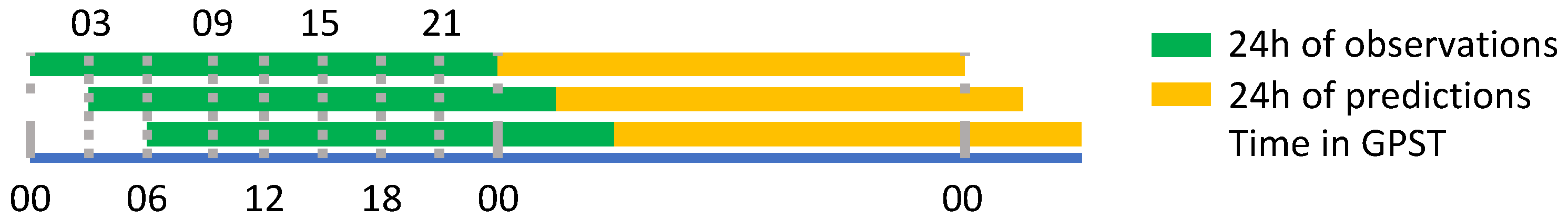
2. Data
3. Methodology
3.1. Overview
3.2. Data Preprocessing
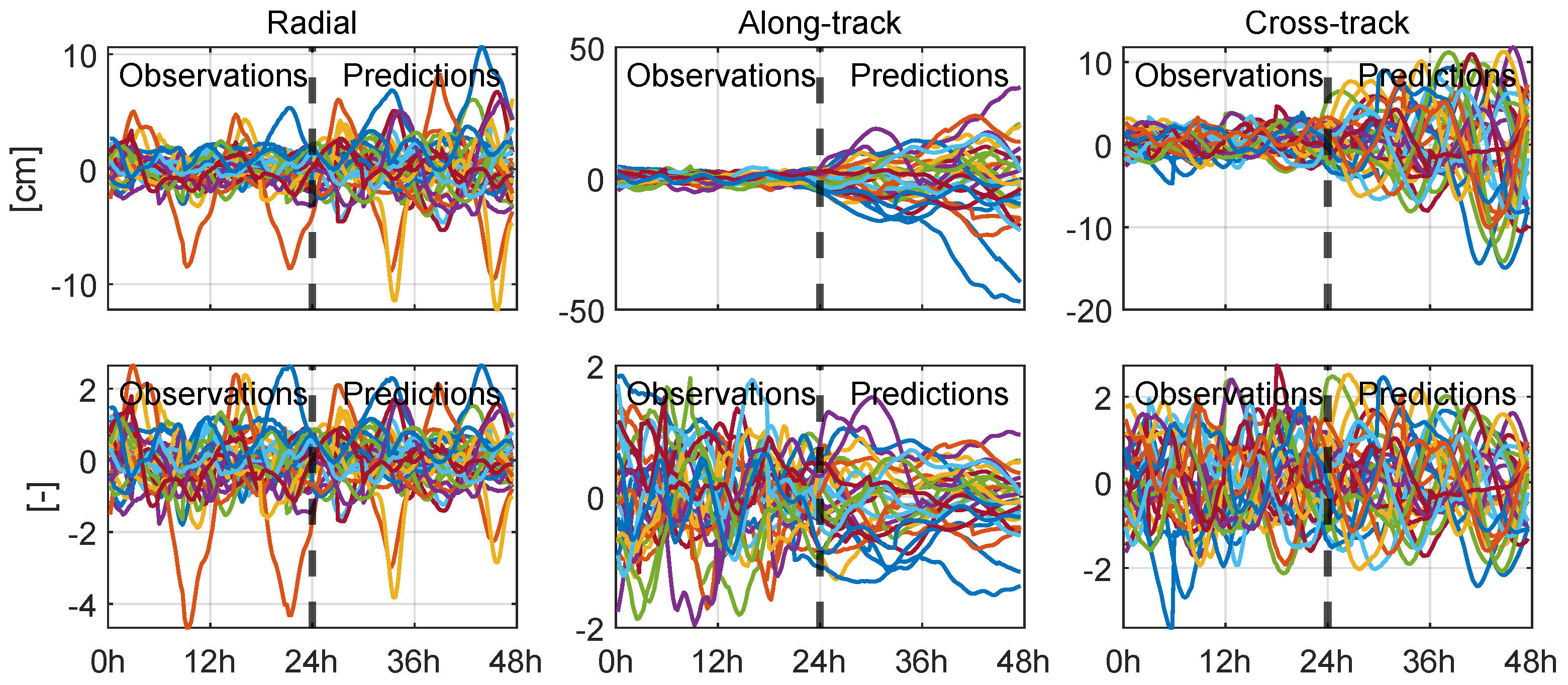
3.2.1. Generating Orbit Differences
3.2.2. Feature Standardization
3.3. Machine-Learning and Deep-Learning Algorithms
3.3.1. Tree-Based Models
3.3.2. Multilayer Perceptron
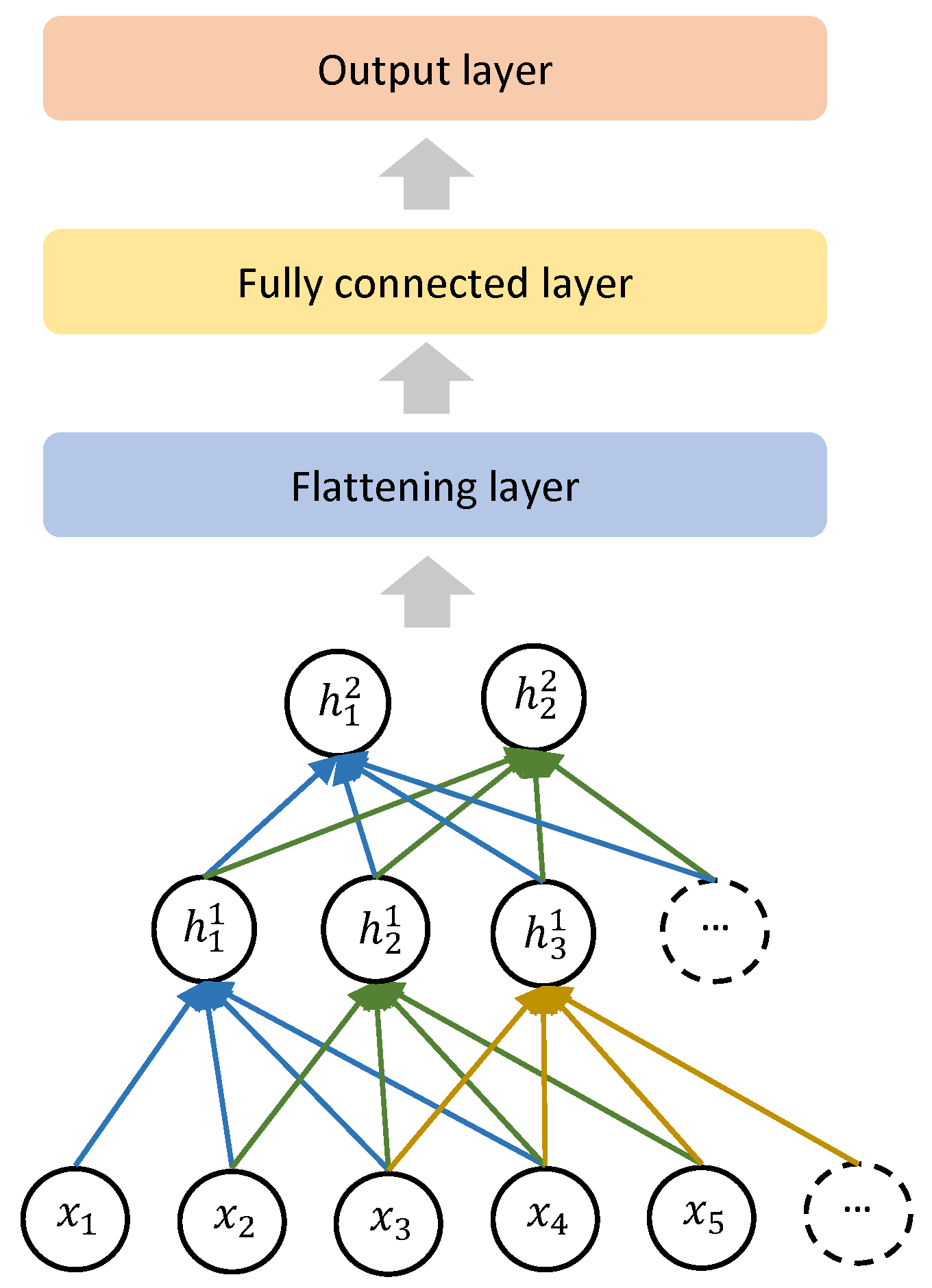
3.3.3. Convolutional Neural Networks
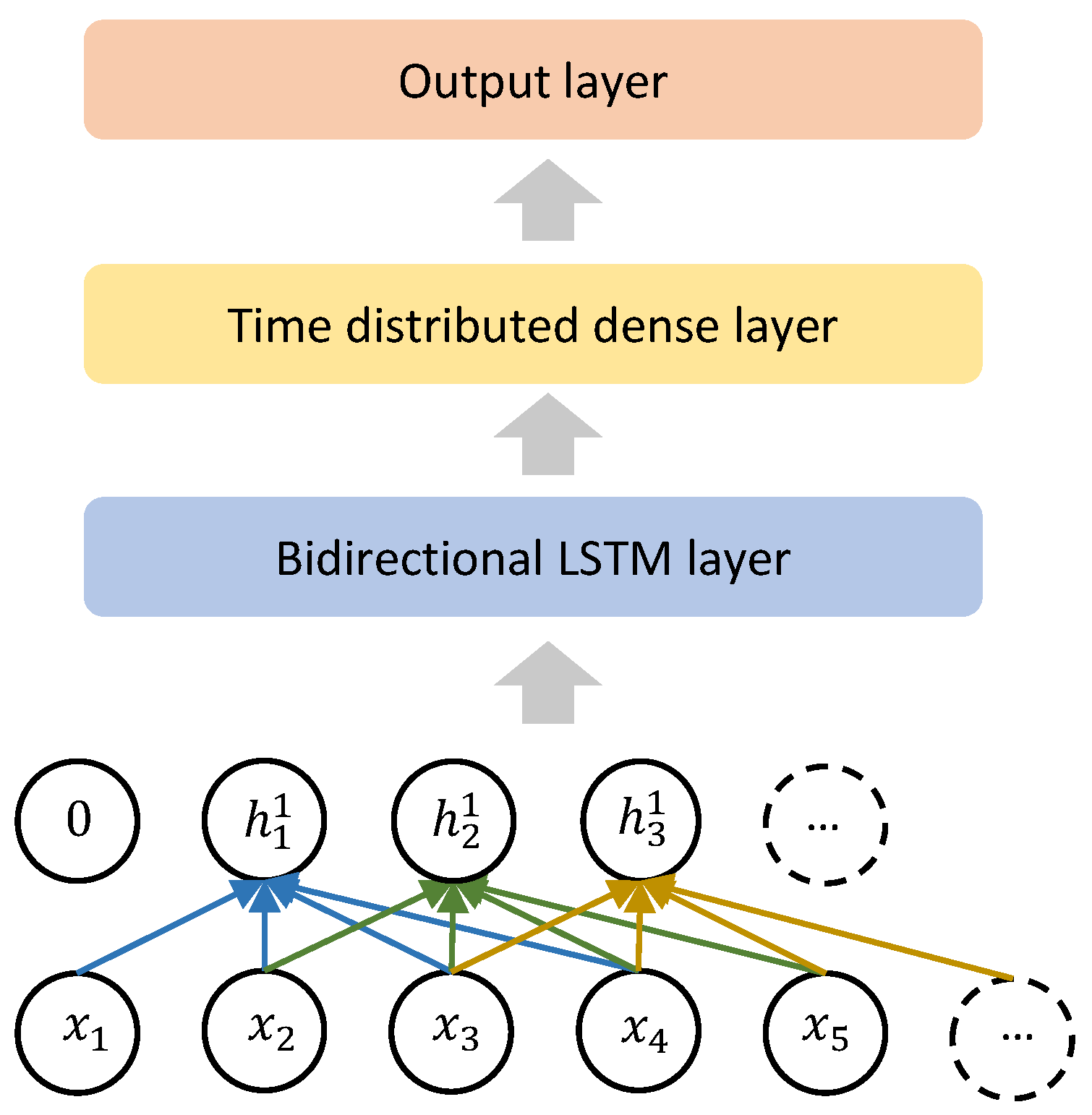
3.3.4. Recurrent Neural Networks
3.3.5. Combination of CNN and LSTM
3.4. Evaluation Metrics
3.5. Kinematic Precise Point Positioning Using Improved Orbits
4. Results and Discussion
4.1. Comparison of Different LSTM Architectures
4.2. Comparison of Machine-Learning and Deep-Learning Models
4.3. Precise Point Positioning Using LSTM-Improved Orbits
5. Conclusions and Outlook
Author Contributions
Funding
Data Availability Statement
Acknowledgments
Conflicts of Interest
Appendix A. Model Architectures

| Model | Layer | Output Shape | Number of Parameters |
|---|---|---|---|
| CNN | Conv1D | (None, 92, 16) | 208 |
| Conv1D | (None, 89, 16) | 1040 | |
| Flatten | (None, 1424) | 0 | |
| Dense | (None, 64) | 91,200 | |
| Dense | (None, 95) | 6175 | |
| LSTM-s2s | LSTM | (None, 95, 128) | 67,584 |
| LSTM | (None, 95, 64) | 49,408 | |
| LSTM | (None, 95, 32) | 12,416 | |
| TimeDistributed(Dense) | (None, 95, 32) | 1056 | |
| TimeDistributed(Dense) | (None, 95, 1) | 33 | |
| biLSTM | Bidirectional(LSTM) | (None, 95, 256) | 135,168 |
| Bidirectional(LSTM) | (None, 95, 128) | 164,352 | |
| Bidirectional(LSTM) | (None, 95, 64) | 41,216 | |
| TimeDistributed(Dense) | (None, 95, 32) | 2080 | |
| TimeDistributed(Dense) | (None, 95, 1) | 33 | |
| LSTM-s2o | LSTM | (None, 95, 128) | 67,584 |
| LSTM | (None, 95, 64) | 49,408 | |
| LSTM | (None, 32) | 12,416 | |
| Dense | (None, 128) | 4224 | |
| Dense | (None, 95) | 12,255 | |
| EDLSTM | LSTM | (None, 95, 128) | 67,584 |
| LSTM | (None, 128) | 131,584 | |
| RepeatVector | (None, 95, 128) | 0 | |
| LSTM | (None, 95, 64) | 49,408 | |
| TimeDistributed(Dense) | (None, 95, 64) | 4160 | |
| TimeDistributed(Dense) | (None, 95, 1) | 65 | |
| CNNLSTM | Conv1D | (None, 95, 4) | 52 |
| Conv1D | (None, 95, 8) | 136 | |
| Conv1D | (None, 95, 16) | 528 | |
| Bidirectional(LSTM) | (None, 95, 60) | 11,280 | |
| Bidirectional(LSTM) | (None, 95, 25) | 8400 | |
| Bidirectional(LSTM) | (None, 95, 14) | 2016 | |
| TimeDistributed(Dense) | (None, 95, 1) | 15 |
References
- Shi, J.; Wang, G.; Han, X.; Guo, J. Impacts of satellite orbit and clock on real-time GPS point and relative positioning. Sensors 2017, 17, 1363. [Google Scholar] [CrossRef] [PubMed]
- Li, H.; Liao, X.; Li, B.; Yang, L. Modeling of the GPS satellite clock error and its performance evaluation in precise point positioning. Adv. Space Res. 2018, 62, 845–854. [Google Scholar] [CrossRef]
- Li, H.; Li, X.; Gong, X. Improved method for the GPS high-precision real-time satellite clock error service. GPS Solut. 2022, 26, 136. [Google Scholar] [CrossRef]
- Li, H.; Li, X.; Xiao, J. Estimating GNSS satellite clock error to provide a new final product and real-time services. GPS Solut. 2024, 28, 17. [Google Scholar] [CrossRef]
- Hauschild, A.; Montenbruck, O. Precise real-time navigation of LEO satellites using GNSS broadcast ephemerides. Navig. J. Inst. Navig. 2021, 68, 419–432. [Google Scholar] [CrossRef]
- Montenbruck, O.; Kunzi, F.; Hauschild, A. Performance assessment of GNSS-based real-time navigation for the Sentinel-6 spacecraft. GPS Solut. 2022, 26, 12. [Google Scholar] [CrossRef]
- Müller, L.; Chen, K.; Möller, G.; Rothacher, M.; Soja, B.; Lopez, L. Real-time navigation solutions of low-cost off-the-shelf GNSS receivers on board the Astrocast constellation satellites. Adv. Space Res. 2023. [Google Scholar] [CrossRef]
- Bergen, K.J.; Johnson, P.A.; Maarten, V.; Beroza, G.C. Machine learning for data-driven discovery in solid Earth geoscience. Science 2019, 363, eaau0323. [Google Scholar] [CrossRef]
- Reichstein, M.; Camps-Valls, G.; Stevens, B.; Jung, M.; Denzler, J.; Carvalhais, N.; Prabhat, F. Deep learning and process understanding for data-driven Earth system science. Nature 2019, 566, 195–204. [Google Scholar] [CrossRef]
- Yu, S.; Ma, J. Deep learning for geophysics: Current and future trends. Rev. Geophys. 2021, 59, e2021RG000742. [Google Scholar] [CrossRef]
- Butt, J.; Wieser, A.; Gojcic, Z.; Zhou, C. Machine learning and geodesy: A survey. J. Appl. Geod. 2021, 15, 117–133. [Google Scholar] [CrossRef]
- Pihlajasalo, J.; Leppäkoski, H.; Ali-Löytty, S.; Piché, R. Improvement of GPS and BeiDou extended orbit predictions with CNNs. In Proceedings of the 2018 European Navigation Conference (ENC), Gothenburg, Sweden, 14–17 May 2018; pp. 54–59. [Google Scholar] [CrossRef]
- Chen, H.; Niu, F.; Su, X.; Geng, T.; Liu, Z.; Li, Q. Initial results of modeling and improvement of BDS-2/GPS broadcast ephemeris satellite orbit based on BP and PSO-BP neural networks. Remote. Sens. 2021, 13, 4801. [Google Scholar] [CrossRef]
- Kiani, M. Simultaneous approximation of a function and its derivatives by Sobolev polynomials: Applications in satellite geodesy and precise orbit determination for LEO CubeSats. Geod. Geodyn. 2020, 11, 376–390. [Google Scholar] [CrossRef]
- Peng, H.; Bai, X. Improving orbit prediction accuracy through supervised machine learning. Adv. Space Res. 2018, 61, 2628–2646. [Google Scholar] [CrossRef]
- Peng, H.; Bai, X. Machine learning approach to improve satellite orbit prediction accuracy using publicly available data. J. Astronaut. Sci. 2020, 67, 762–793. [Google Scholar] [CrossRef]
- Mortlock, T.; Kassas, Z.M. Assessing machine learning for LEO satellite orbit determination in simultaneous tracking and navigation. In Proceedings of the 2021 IEEE Aerospace Conference (50100), Big Sky, MT, USA, 6–13 March 2021; pp. 1–8. [Google Scholar] [CrossRef]
- Johnston, G.; Riddell, A.; Hausler, G. The International GNSS Service. In Springer Handbook of Global Navigation Satellite Systems; Springer International Publishing: Cham, Switzerland, 2017; pp. 967–982. [Google Scholar] [CrossRef]
- Duan, B.; Hugentobler, U.; Chen, J.; Selmke, I.; Wang, J. Prediction versus real-time orbit determination for GNSS satellites. GPS Solut. 2019, 23, 1–10. [Google Scholar] [CrossRef]
- Wang, Q.; Hu, C.; Xu, T.; Chang, G.; Moraleda, A.H. Impacts of Earth rotation parameters on GNSS ultra-rapid orbit prediction: Derivation and real-time correction. Adv. Space Res. 2017, 60, 2855–2870. [Google Scholar] [CrossRef]
- IGS Products. Available online: https://igs.org/products/#orbits_clocks (accessed on 24 November 2012).
- Männel, B.; Brandt, A.; Nischan, T.; Brack, A.; Sakic, P.; Bradke, M. GFZ Ultra-Rapid Product Series for the International GNSS Service (IGS); GFZ Data Services: Potsdam, Germany, 2020. [Google Scholar] [CrossRef]
- Männel, B.; Brandt, A.; Nischan, T.; Brack, A.; Sakic, P.; Bradke, M. GFZ Final Product Series for the International GNSS Service (IGS); GFZ Data Services: Potsdam, Germany, 2020. [Google Scholar] [CrossRef]
- Griffiths, J. Combined orbits and clocks from IGS second reprocessing. J. Geod. 2019, 93, 177–195. [Google Scholar] [CrossRef]
- Rothacher, M. Orbits of Satellite Systems in Space Geodesy; lnstitut ftlr Geodlsie mid Photogrammetrie: Zurich, Switzerland, 1992; Volume 46. [Google Scholar]
- Petit, G.; Luzum, B. IERS Conventions (2010); Verlag des Bundesamts für Kartographie und Geodäsie: Frankfurt, Germany, 2010. [Google Scholar]
- Montenbruck, O.; Gill, E. Satellite Orbits: Models, Methods and Applications; Springer Science & Business Media: Berlin/Heidelberg, Germany, 2012. [Google Scholar]
- Goodfellow, I.; Bengio, Y.; Courville, A. Deep Learning; MIT Press: Cambridge, MA, USA, 2016. [Google Scholar]
- Pedregosa, F.; Varoquaux, G.; Gramfort, A.; Michel, V.; Thirion, B.; Grisel, O.; Blondel, M.; Prettenhofer, P.; Weiss, R.; Dubourg, V.; et al. Scikit-learn: Machine Learning in Python. J. Mach. Learn. Res. 2011, 12, 2825–2830. [Google Scholar]
- Crocetti, L.; Schartner, M.; Soja, B. Discontinuity Detection in GNSS Station Coordinate Time Series Using Machine Learning. Remote. Sens. 2021, 13, 3906. [Google Scholar] [CrossRef]
- Jing, W.; Zhao, X.; Yao, L.; Di, L.; Yang, J.; Li, Y.; Guo, L.; Zhou, C. Can terrestrial water storage dynamics be estimated from climate anomalies? Earth Space Sci. 2020, 7, e2019EA000959. [Google Scholar] [CrossRef]
- Kiani Shahvandi, M.; Gou, J.; Schartner, M.; Soja, B. Data Driven Approaches for the Prediction of Earth’s Effective Angular Momentum Functions. In Proceedings of the IGARSS 2022—2022 IEEE International Geoscience and Remote Sensing Symposium, Kuala Lumpur, Malaysia, 17–22 July 2022; pp. 6550–6553. [Google Scholar] [CrossRef]
- Breiman, L. Classification and Regression Trees; Wiley Interdisciplinary Reviews: Data Mining and Knowledge Discovery; Routledge: New York, NY, USA, 2011; Volume 1, pp. 14–23. [Google Scholar] [CrossRef]
- Breiman, L. Random forests. Mach. Learn. 2001, 45, 5–32. [Google Scholar] [CrossRef]
- Močkus, J. On bayesian methods for seeking the extremum. In Proceedings of the Optimization Techniques IFIP Technical Conference, Novosibirsk, Russia, 1–7 July 1974; Marchuk, G.I., Ed.; Springer: Berlin/Heidelberg, Germany, 1975; pp. 400–404. [Google Scholar] [CrossRef]
- Snoek, J.; Larochelle, H.; Adams, R.P. Practical Bayesian Optimization of Machine Learning Algorithms. In Proceedings of the Advances in Neural Information Processing Systems, Lake Tahoe, NV, USA, 3–8 December 2012; Pereira, F., Burges, C., Bottou, L., Weinberger, K., Eds.; Curran Associates, Inc.: New York, NY, USA, 2012; Volume 25. [Google Scholar]
- Haykin, S. Neural Networks: A Comprehensive Foundation; Prentice Hall PTR: Hoboken, NJ, USA, 1994. [Google Scholar]
- Schuh, H.; Ulrich, M.; Egger, D.; Müller, J.; Schwegmann, W. Prediction of Earth orientation parameters by artificial neural networks. J. Geod. 2002, 76, 247–258. [Google Scholar] [CrossRef]
- Li, F.; Kusche, J.; Rietbroek, R.; Wang, Z.; Forootan, E.; Schulze, K.; Lück, C. Comparison of data-driven techniques to reconstruct (1992–2002) and predict (2017–2018) GRACE-like gridded total water storage changes using climate inputs. Water Resour. Res. 2020, 56, e2019WR026551. [Google Scholar] [CrossRef]
- LeCun, Y.; Bottou, L.; Bengio, Y.; Haffner, P. Gradient-based learning applied to document recognition. Proc. IEEE 1998, 86, 2278–2324. [Google Scholar] [CrossRef]
- Abadi, M.; Agarwal, A.; Barham, P.; Brevdo, E.; Chen, Z.; Citro, C.; Corrado, G.S.; Davis, A.; Dean, J.; Devin, M.; et al. TensorFlow: Large-Scale Machine Learning on Heterogeneous Systems. 2015. Available online: tensorflow.org (accessed on 1 March 2021).
- Rumelhart, D.E.; Hinton, G.E.; Williams, R.J. Learning representations by back-propagating errors. Nature 1986, 323, 533–536. [Google Scholar] [CrossRef]
- Bengio, Y.; Simard, P.; Frasconi, P. Learning long-term dependencies with gradient descent is difficult. IEEE Trans. Neural Netw. 1994, 5, 157–166. [Google Scholar] [CrossRef] [PubMed]
- Pascanu, R.; Mikolov, T.; Bengio, Y. On the difficulty of training recurrent neural networks. In Proceedings of the International Conference on Machine Learning, PMLR, Atlanta, GA, USA, 16–21 June 2013; pp. 1310–1318. [Google Scholar]
- Hochreiter, S.; Schmidhuber, J. Long Short-Term Memory. Neural Comput. 1997, 9, 1735–1780. [Google Scholar] [CrossRef]
- Gou, J.; Kiani Shahvandi, M.; Hohensinn, R.; Soja, B. Ultra-short-term prediction of LOD using LSTM neural networks. J. Geod. 2023, 97, 52. [Google Scholar] [CrossRef]
- Kiani Shahvandi, M.; Soja, B. Small geodetic datasets and deep networks: Attention-based residual LSTM Autoencoder stacking for geodetic time series. In Proceedings of the 7th International Conference on Machine Learning, Optimization, and Data Science, Grasmere, UK, 4–8 October 2021. [Google Scholar] [CrossRef]
- Kiani Shahvandi, M.; Soja, B. Inclusion of data uncertainty in machine learning and its application in geodetic data science, with case studies for the prediction of Earth orientation parameters and GNSS station coordinate time series. Adv. Space Res. 2022, 70, 563–575. [Google Scholar] [CrossRef]
- Tang, J.; Li, Y.; Ding, M.; Liu, H.; Yang, D.; Wu, X. An ionospheric TEC forecasting model based on a CNN-LSTM-attention mechanism neural network. Remote. Sens. 2022, 14, 2433. [Google Scholar] [CrossRef]
- Cho, K.; Van Merriënboer, B.; Gulcehre, C.; Bahdanau, D.; Bougares, F.; Schwenk, H.; Bengio, Y. Learning phrase representations using RNN encoder-decoder for statistical machine translation. arXiv 2014, arXiv:1406.1078. [Google Scholar]
- Sutskever, I.; Vinyals, O.; Le, Q.V. Sequence to sequence learning with neural networks. In Proceedings of the Advances in Neural Information Processing Systems, Montreal, QC, Canada, 8–13 October 2014. pp. 3104–3112.
- Donahue, J.; Anne Hendricks, L.; Guadarrama, S.; Rohrbach, M.; Venugopalan, S.; Saenko, K.; Darrell, T. Long-term recurrent convolutional networks for visual recognition and description. In Proceedings of the IEEE Conference on Computer Vision and Pattern Recognition, Boston, MA, USA, 7–12 June 2015; pp. 2625–2634. [Google Scholar]
- Dach, R.; Lutz, S.; Walser, P.; Fridez, P. Bernese GNSS Software, version 5.2; Astronomical Institute, University of Bern: Bern, Switzerland. [CrossRef]
- Böhm, J.; Heinkelmann, R.; Schuh, H. Short note: A global model of pressure and temperature for geodetic applications. J. Geod. 2007, 81, 679–683. [Google Scholar] [CrossRef]
- Dach, R.; Schaer, S.; Arnold, D.; Kalarus, M.S.; Prange, L.; Stebler, P.; Villiger, A.; Jäggi, A. CODE Final Product Series for the IGS; Astronomical Institute, University of Bern: Bern, Switzerland, 2020. [Google Scholar] [CrossRef]
- Chen, K.; Xu, T.; Yang, Y. Robust combination of IGS analysis center GLONASS clocks. GPS Solut. 2017, 21, 1251–1263. [Google Scholar] [CrossRef]
- IGS. International GNSS Service, GNSS Final Cumulative Combined Set of Station Coordinates Product, Greenbelt, MD, USA: NASA Crustal Dynamics Data Information System (CDDIS). 2022. Available online: https://cddis.nasa.gov/Data_and_Derived_Products/GNSS/gnss_igssnx.html (accessed on 16 May 2022).
- Noll, C.E. The crustal dynamics data information system: A resource to support scientific analysis using space geodesy. Adv. Space Res. 2010, 45, 1421–1440. [Google Scholar] [CrossRef]
- Santerre, R. Impact of GPS satellite sky distribution. Manuscripta Geod. 1991, 16, 28–53. [Google Scholar]
- Lutz, S.; Beutler, G.; Schaer, S.; Dach, R.; Jäggi, A. CODE’s new ultra-rapid orbit and ERP products for the IGS. GPS Solut. 2016, 20, 239–250. [Google Scholar] [CrossRef]


| Radial | Along-Track | Cross-Track | 3D | |||||||||
|---|---|---|---|---|---|---|---|---|---|---|---|---|
| Max. | Ave. | Min. | Max. | Ave. | Min. | Max. | Ave. | Min. | Max. | Ave. | Min. | |
| LSTM-s2s | 1.8 | 0.8 | 0.3 | 10.4 | 3.1 | 0 | 1.8 | 0.6 | 0 | 10.7 | 3.3 | 0.2 |
| biLSTM | 1.8 | 1.3 | 1.1 | 14.3 | 8.9 | 3.3 | 1.9 | 1.0 | 0.6 | 14.5 | 8.9 | 3.8 |
| LSTM-s2o | 1.8 | 1.3 | 1.1 | 16.7 | 9.7 | 3.8 | 2.0 | 1.1 | 0.7 | 16.8 | 9.7 | 4.3 |
| EDLSTM | 1.9 | 1.3 | 1.0 | 14.5 | 9.0 | 3.9 | 1.8 | 1.1 | 0.6 | 14.7 | 9.0 | 4.4 |
| Model | Radial | Along-Track | Cross-Track | 3D |
|---|---|---|---|---|
| LSTM-s2s | 81 | 63 | 68 | 70 |
| LSTM-s2o | 88 | 70 | 75 | 77 |
| biLSTM | 89 | 70 | 74 | 77 |
| EDLSTM | 88 | 70 | 75 | 77 |
| Radial | Along-Track | Cross-Track | 3D | |||||||||
|---|---|---|---|---|---|---|---|---|---|---|---|---|
| Max. | Ave. | Min. | Max. | Ave. | Min. | Max. | Ave. | Min. | Max. | Ave. | Min. | |
| DT | 0.9 | 0.5 | 0.1 | 9.0 | 3.7 | 1.7 | 1.1 | 0.5 | 0.2 | 9.0 | 3.8 | 1.7 |
| RF | 1.1 | 0.5 | 0.2 | 12.7 | 5.0 | 1.9 | 1.4 | 0.7 | 0.2 | 12.8 | 5.0 | 2.0 |
| MLP | 1.3 | 0.8 | 0.3 | 14.2 | 9.1 | 5.0 | 1.4 | 1.0 | 0.4 | 14.3 | 9.1 | 5.3 |
| CNN | 1.5 | 1.0 | 0.7 | 13.0 | 7.6 | 2.7 | 1.9 | 1.0 | 0.5 | 13.2 | 7.6 | 3.3 |
| LSTM-s2o | 1.8 | 1.3 | 1.1 | 16.7 | 9.7 | 3.8 | 2.0 | 1.1 | 0.7 | 16.8 | 9.7 | 4.3 |
| CNNLSTM | 1.8 | 1.2 | 0.9 | 14.0 | 8.9 | 3.2 | 1.9 | 1.0 | 0.5 | 14.2 | 8.9 | 3.7 |
| Model | Radial | Along-Track | Cross-Track | 3D |
|---|---|---|---|---|
| DT | 73 | 61 | 67 | 67 |
| RF | 83 | 66 | 72 | 73 |
| MLP | 81 | 66 | 73 | 74 |
| CNN | 86 | 70 | 73 | 76 |
| LSTM-s2o | 88 | 70 | 75 | 77 |
| CNNLSTM | 88 | 72 | 75 | 78 |
Disclaimer/Publisher’s Note: The statements, opinions and data contained in all publications are solely those of the individual author(s) and contributor(s) and not of MDPI and/or the editor(s). MDPI and/or the editor(s) disclaim responsibility for any injury to people or property resulting from any ideas, methods, instructions or products referred to in the content. |
© 2023 by the authors. Licensee MDPI, Basel, Switzerland. This article is an open access article distributed under the terms and conditions of the Creative Commons Attribution (CC BY) license (https://creativecommons.org/licenses/by/4.0/).
Share and Cite
Gou, J.; Rösch, C.; Shehaj, E.; Chen, K.; Kiani Shahvandi, M.; Soja, B.; Rothacher, M. Modeling the Differences between Ultra-Rapid and Final Orbit Products of GPS Satellites Using Machine-Learning Approaches. Remote Sens. 2023, 15, 5585. https://doi.org/10.3390/rs15235585
Gou J, Rösch C, Shehaj E, Chen K, Kiani Shahvandi M, Soja B, Rothacher M. Modeling the Differences between Ultra-Rapid and Final Orbit Products of GPS Satellites Using Machine-Learning Approaches. Remote Sensing. 2023; 15(23):5585. https://doi.org/10.3390/rs15235585
Chicago/Turabian StyleGou, Junyang, Christine Rösch, Endrit Shehaj, Kangkang Chen, Mostafa Kiani Shahvandi, Benedikt Soja, and Markus Rothacher. 2023. "Modeling the Differences between Ultra-Rapid and Final Orbit Products of GPS Satellites Using Machine-Learning Approaches" Remote Sensing 15, no. 23: 5585. https://doi.org/10.3390/rs15235585
APA StyleGou, J., Rösch, C., Shehaj, E., Chen, K., Kiani Shahvandi, M., Soja, B., & Rothacher, M. (2023). Modeling the Differences between Ultra-Rapid and Final Orbit Products of GPS Satellites Using Machine-Learning Approaches. Remote Sensing, 15(23), 5585. https://doi.org/10.3390/rs15235585