


Learn by Yourself: A Feature-Augmented Self-Distillation Convolutional Neural Network for Remote Sensing Scene Image Classification


Abstract
:1. Introduction
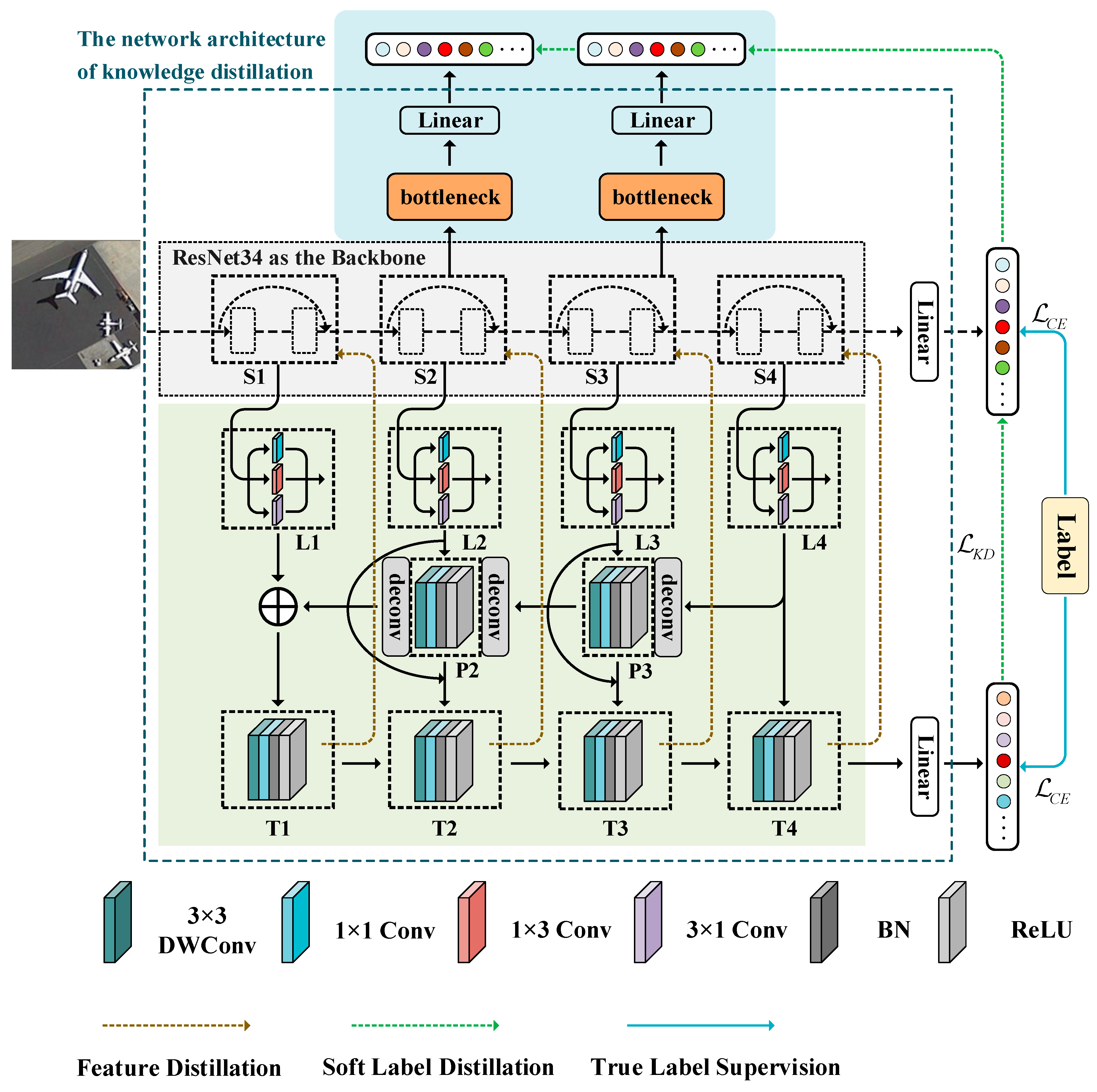
- This paper proposes a new self-distillation framework that effectively combines feature distillation and logits distillation to solve the problem of losing fine-grained information in traditional hard-label supervised models. This enables the backbone network to extract more representative features of the image and improve the generalization performance and adversarial nature of the model. Extensive experiments on four commonly used remote sensing scene image classification datasets have demonstrated the effectiveness of the proposed method.
- In order to complement the advantages of multi-level features, a feature augmentation pyramid module is carefully designed, which fuses the top-level features with the low-level features through deconvolution to increase the richness of the features, so that the semantic features extracted by the deep network can be learned by the underlying network.
- A method of adding two auxiliary classifiers in the middle layer is proposed, which is trained through distillation to provide additional supervisory information and help the network converge faster. In order to ensure that the shallow auxiliary classifier and the main classifier share similar feature representations, a bottleneck structure is added to the middle layer of the backbone network to encourage them to learn similar features.
2. Related Works
2.1. Classification of Remote Sensing Scene Images
2.2. Knowledge Distillation
3. Methodology
3.1. Self-Distillation
3.2. Feature Augmentation Pyramid Module (FAPM)
3.3. Auxiliary Classifier
3.4. Implementation Details
| Algorithm 1. The process of the proposed FASDNet |
|
4. Experiments
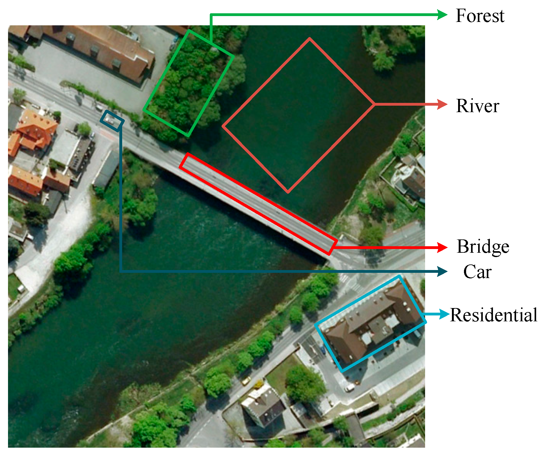
4.1. Datasets
- (1)
- UC-Merced
- (2)
- RSSCN7
- (3)
- AID
- (4)
- NWPU-RESISC45
4.2. Experimental Details
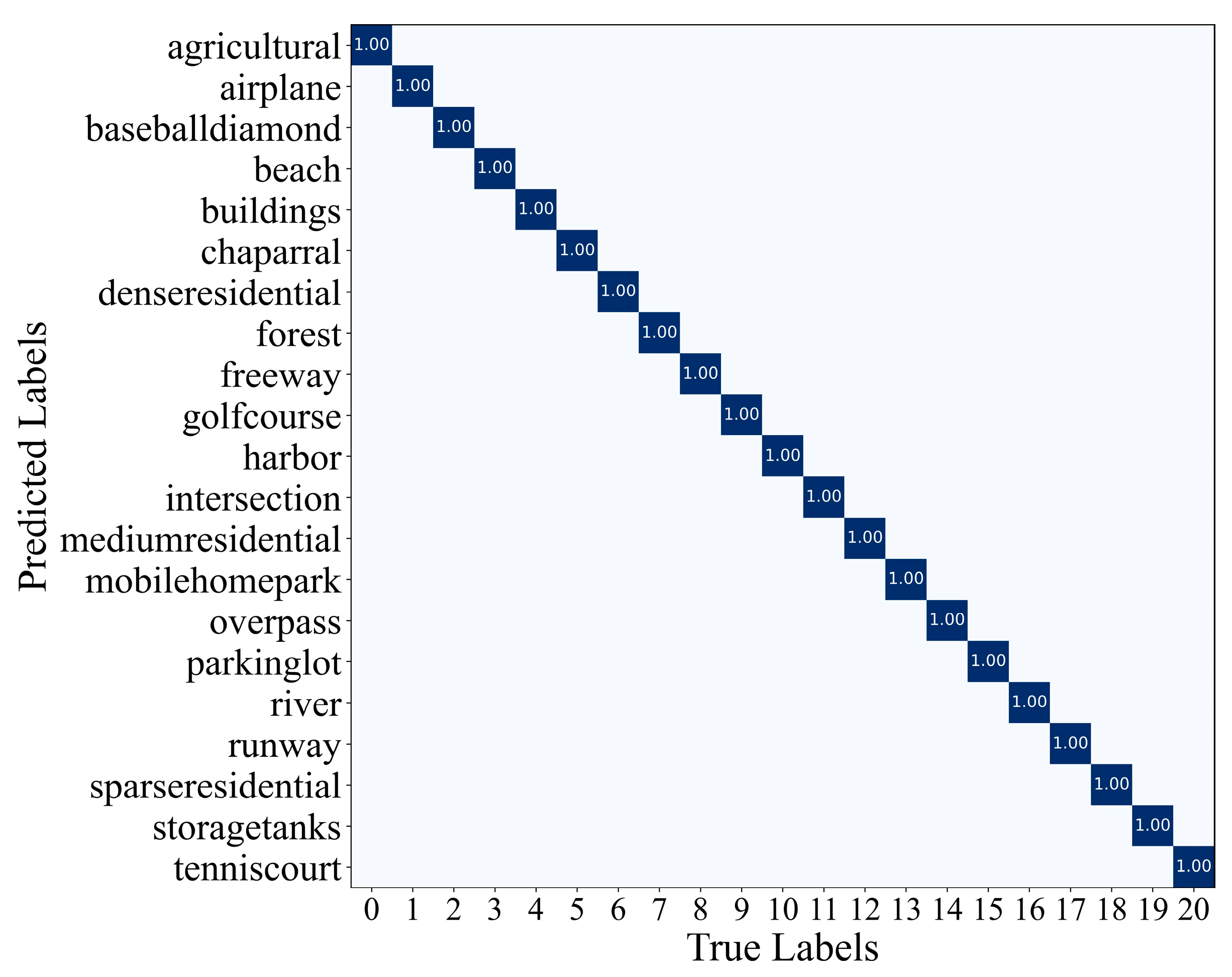
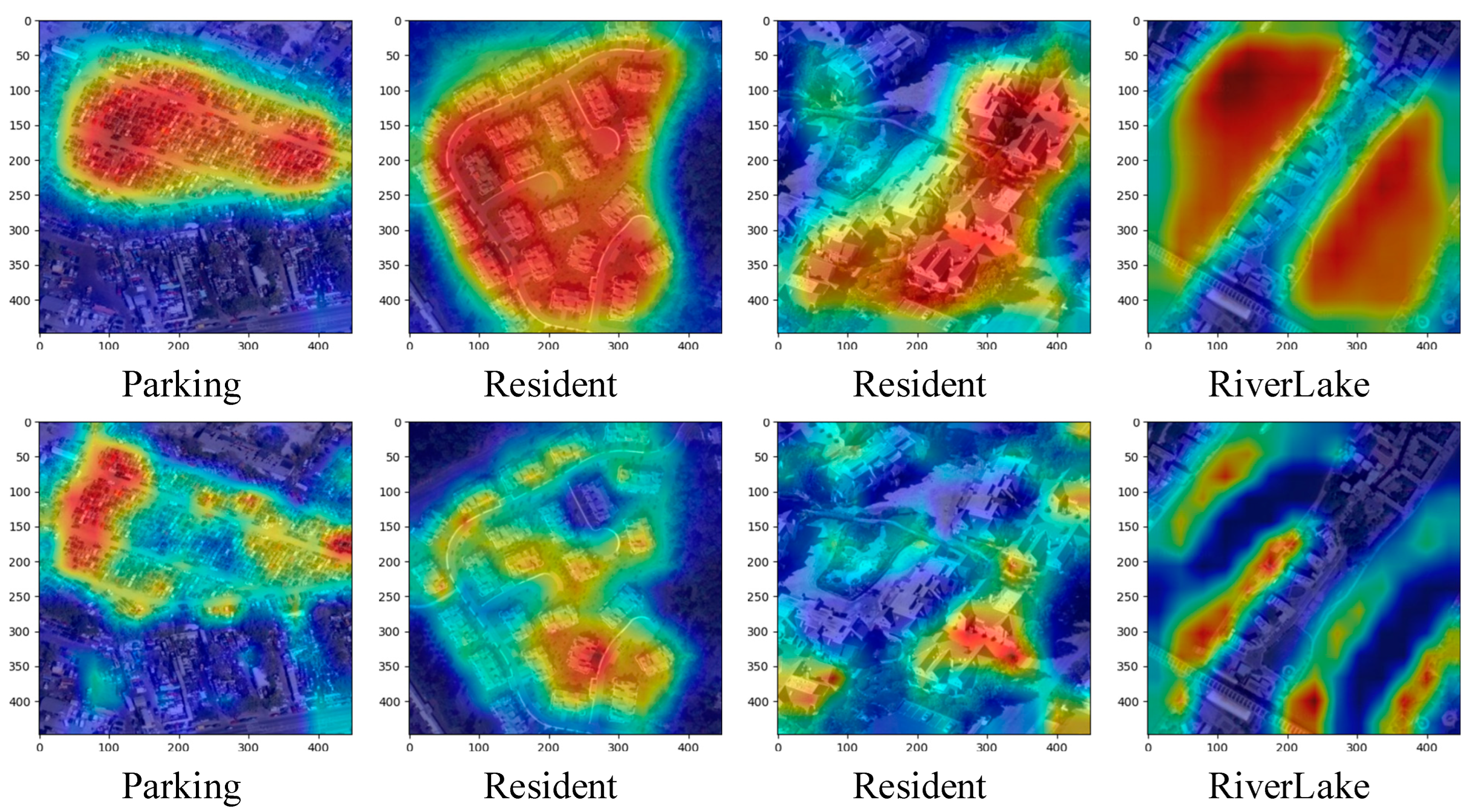
4.3. Experimental Results and Analysis
- (1)
- Classification results on the UC-Merced dataset
- (2)
- Classification results on the RSSCN7 dataset
- (3)
- Classification results on the AID:
- (4)
- Classification results on the NWPU dataset:
4.4. Evaluation of Size of Models
4.5. Discussion
5. Conclusions
Author Contributions
Funding
Acknowledgments
Conflicts of Interest
References
- Jaiswal, R.K.; Saxena, R.; Mukherjee, S. Application of remote sensing technology for land use/land cover change analysis. J. Indian Soc. Remote Sens. 1999, 27, 123–128. [Google Scholar] [CrossRef]
- Chova, L.G.; Tuia, D.; Moser, G.; Valls, G.C. Multimodal classification of remote sensing images: A review and future directions. IEEE Proc. 2015, 103, 1560–1584. [Google Scholar] [CrossRef]
- Cheng, G.; Zhou, P.; Han, J. Learning Rotation-Invariant Convolutional Neural Networks for Object Detection in VHR Optical Remote Sensing Images. IEEE Trans. Geosci. Remote Sens. 2016, 54, 7405–7415. [Google Scholar] [CrossRef]
- Zhang, L.; Zhang, L.; Du, B. Deep learning for remote sensing data: A technical tutorial on the state-of-the-art. IEEE Geosci. Remote Sens. Mag. 2016, 4, 22–40. [Google Scholar] [CrossRef]
- Grigorescu, S.E.; Petkov, N.; Kruizinga, P. Comparison of texture features based on Gabor filters. IEEE Trans. Image Process. 2002, 11, 1160–1167. [Google Scholar] [CrossRef] [PubMed]
- Tang, X.; Jiao, L.; Emery, W.J. SAR image content retrieval based on fuzzy similarity and relevance feedback. IEEE J. Sel. Topics Appl. Earth Observ. Remote Sens. 2017, 10, 1824–1842. [Google Scholar] [CrossRef]
- Mei, S.; Ji, J.; Hou, J.; Li, X.; Du, Q. Learning sensor-specific spatial–spectral features of hyperspectral images via convolutional neural networks. IEEE Trans. Geosci. Remote Sens. 2017, 55, 4520–4533. [Google Scholar] [CrossRef]
- Jiao, L.; Tang, X.; Hou, B.; Wang, S. SAR images retrieval based on semantic classification and region-based similarity measure for Earth observation. IEEE J. Sel. Topics Appl. Earth Observ. Remote Sens. 2015, 8, 3876–3891. [Google Scholar] [CrossRef]
- Sergyan, S. Color histogram features based image classification in content-based image retrieval systems. In Proceedings of the 6th International Symposium on Applied Machine Intelligence and Informatics, Herlany, Slovakia, 21–22 January 2008; pp. 221–224. [Google Scholar]
- Tang, X.; Jiao, L. Fusion similarity-based reranking for SAR image retrieval. IEEE Geosci. Remote Sens. Lett. 2017, 14, 242–246. [Google Scholar] [CrossRef]
- Soltanian-Zadeh, H.; Rafiee-Rad, F.; Pourabdollah-Nejad, S. Comparison of multiwavelet, wavelet, haralick, and shape features for microcalcification classification in mammograms. Pattern Recognit. 2004, 37, 1973–1986. [Google Scholar] [CrossRef]
- Tang, X.; Jiao, L.; Emery, W.J.; Liu, F.; Zhang, D. Two-stage reranking for remote sensing image retrieval. IEEE Trans. Geosci. Remote Sens. 2017, 55, 5798–5817. [Google Scholar] [CrossRef]
- Zhang, L.; Zhou, W.; Jiao, L. Wavelet support vector machine. IEEE Trans. Syst. Man Cybern. B Cybern. 2004, 34, 34–39. [Google Scholar] [CrossRef] [PubMed]
- Friedl, M.A.; Brodley, C.E. Decision tree classification of land cover from remotely sensed data. Remote Sens. Environ. 1997, 61, 399–409. [Google Scholar] [CrossRef]
- Khan; Sohail, A.; Zahoora, U.; Qureshi, A.S. A survey of the recent architectures of deep convolutional neural networks. Artif. Intell. Rev. 2020, 53, 5455–5516. [Google Scholar] [CrossRef]
- Zhu, G.; Shu, J. Robust Joint Representation of Intrinsic Mean and Kernel Function of Lie Group for Remote Sensing Scene Classification. IEEE Geosci. Remote Sens. Lett. 2021, 18, 796–800. [Google Scholar] [CrossRef]
- Liu, M.; Jiao, L.; Liu, X.; Li, L.; Liu, F.; Yang, S. C-CNN: Contourlet Convolutional Neural Networks. IEEE Trans. Neural Netw. Learn. Syst. 2021, 32, 2636–2649. [Google Scholar] [CrossRef]
- Zhang, D.; Li, N.; Ye, Q. Positional Context Aggregation Network for Remote Sensing Scene Classification. IEEE Geosci. Remote Sens. Lett. 2020, 17, 943–947. [Google Scholar] [CrossRef]
- He, N.; Fang, L.; Li, S.; Plaza, J.; Plaza, A. Skip-Connected Covariance Network for Remote Sensing Scene Classification. IEEE Trans. Neural Netw. Learn. Syst. 2020, 31, 1461–1474. [Google Scholar] [CrossRef]
- Hinton, G.; Vinyals, O.; Dean, J. Distilling the Knowledge in a Neural Network. arXiv 2015, arXiv:1503.02531. [Google Scholar]
- Zhang, R.; Li, X.; Liu, W. Self-distillation with label refining for human pose estimation. In Proceedings of the IEEE/CVF Conference on Computer Vision and Pattern Recognition, Seattle, WA, USA, 13–19 June 2020; pp. 10736–10745. [Google Scholar]
- Woloszynski, T.; Ruta, D.; Schaefer, G. Combining multiple classifiers with dynamic classifier selection. Pattern Recognit. 2013, 46, 3054–3066. [Google Scholar]
- Yu, L.; Liu, H.; Motoda, H. Selective ensemble with application to data classification. Inf. Fusion 2014, 15, 17–26. [Google Scholar]
- Dalal, N.; Triggs, B. Histograms of oriented gradients for human detection. In Proceedings of the IEEE Computer Society Conference on Computer Vision and Pattern Recognition (CVPR), San Diego, CA, USA, 20–26 June 2005; Volume 1, pp. 886–893. [Google Scholar]
- Yang, Y.; Newsam, S. Comparing SIFT descriptors and Gabor texture features for classification of remote sensed imagery. In Proceedings of the 15th IEEE International Conference on Image Processing, San Diego, CA, USA, 12–15 October 2008; pp. 1852–1855. [Google Scholar]
- Yang, Y.; Newsam, S. Bag-of-visual-words and spatial extensions for land-use classification. In Proceedings of the 18th SIGSPATIAL International Conference on Advances in Geographic Information Systems (GIS), San Jose, CA, USA, 2–5 November 2010; pp. 270–279. [Google Scholar]
- Li, Y.; Wang, Q.; Liang, X.; Jiao, L. A Novel Deep Feature Fusion Network for Remote Sensing Scene Classification. In Proceedings of the IGARSS 2019—2019 IEEE International Geoscience and Remote Sensing Symposium, Yokohama, Japan, 28 July–2 August 2019; pp. 5484–5487. [Google Scholar]
- Zhao, B.; Zhong, Y.; Xia, G.S.; Zhang, L. Dirichlet-derived multiple topic scene classification model for high spatial resolution remote sensing imagery. IEEE Trans. Geosci. Remote Sens. 2015, 54, 2108–2123. [Google Scholar] [CrossRef]
- Wang, Q.; Liu, S.; Chanussot, J.; Li, X. Scene Classification with Recurrent Attention of VHR Remote Sensing Images. IEEE Trans. Geosci. Remote Sens. 2019, 57, 1155–1167. [Google Scholar] [CrossRef]
- Li, F.; Feng, R.; Han, W.; Wang, L. High-resolution remote sensing image scene classification via key filter bank based on convolutional neural network. IEEE Trans. Geosci. Remote Sens. 2020, 58, 8077–8092. [Google Scholar] [CrossRef]
- Shi, J.; Liu, W.; Shan, H.; Li, E.; Li, X.; Zhang, L. Remote Sensing Scene Classification Based on Multibranch Fusion Attention Network. IEEE Geosci. Remote Sens. Lett. 2023, 20, 3001505. [Google Scholar] [CrossRef]
- Shi, C.; Zhang, X.; Sun, J.; Wang, L. Remote sensing scene image classification based on dense fusion of multi-level features. Remote Sens. 2021, 13, 4379. [Google Scholar] [CrossRef]
- Deng, P.; Huang, H.; Xu, K. A Deep Neural Network Combined with Context Features for Remote Sensing Scene Classification. IEEE Geosci. Remote Sens. Lett. 2022, 19, 8000405. [Google Scholar] [CrossRef]
- Meng, Q.; Zhao, M.; Zhang, L.; Shi, W.; Su, C.; Bruzzone, L. Multilayer Feature Fusion Network with Spatial Attention and Gated Mechanism for Remote Sensing Scene Classification. IEEE Geosci. Remote Sens. Lett. 2022, 19, 6510105. [Google Scholar] [CrossRef]
- Wang, X.; Wang, S.; Ning, C.; Zhou, H. Enhanced feature pyramid network with deep semantic embedding for remote sensing scene classification. IEEE Trans. Geosci. Remote Sens. 2021, 59, 7918–7932. [Google Scholar] [CrossRef]
- Zhang, T.; Wang, Z.; Cheng, P.; Xu, G.; Sun, X. DCNNet: A Distributed Convolutional Neural Network for Remote Sensing Image Classification. IEEE Trans. Geosci. Remote Sens. 2023, 61, 5603618. [Google Scholar] [CrossRef]
- Goodfellow, H.J.I.; Bengio, Y.; Courville, A. Deep learning: The MIT Press, 2016, 800 pp, ISBN: 0262035618. Genet. Program. Evolvable Mach. 2018, 19, 305–307. [Google Scholar]
- Kullback, S.; Leibler, R.A. On information and sufficiency. Ann. Math. Stat. 1951, 22, 79–86. [Google Scholar] [CrossRef]
- Romero, A.; Ballas, N.; Kahou, S.E.; Chassang, A.; Gatta, C.; Bengio, Y. FitNets: Hints for thin deep nets. arXiv 2014, arXiv:1412.6550. [Google Scholar]
- Zagoruyko, S.; Komodakis, N. Paying more attention to attention: Improving the performance of convolutional neural networks via attention transfer. arXiv 2016, arXiv:1612.03928. [Google Scholar]
- Park, W.; Kim, D.; Lu, Y.; Cho, M. Relational knowledge distillation. In Proceedings of the IEEE/CVF Conference on Computer Vision and Pattern Recognition, Long Beach, CA, USA, 16–20 June 2019; pp. 3967–3976. [Google Scholar]
- Heo, B.; Kim, J.; Yun, S.; Park, H.; Kwak, N.; Choi, J.Y. A comprehensive overhaul of feature distillation. In Proceedings of the IEEE/CVF International Conference on Computer Vision, Seoul, Republic of Korea, 27 October–2 November 2019; pp. 1921–1930. [Google Scholar]
- Ahn, S.; Hu, S.X.; Damianou, A.; Lawrence, N.D.; Dai, Z. Variational information distillation for knowledge transfer. In Proceedings of the IEEE/CVF Conference on Computer Vision and Pattern Recognition, Long Beach, CA, USA, 16–20 June 2019; pp. 9163–9171. [Google Scholar]
- Zhang, L.; Song, J.; Gao, A.; Chen, J.; Bao, C.; Ma, K. Be your own teacher: Improve the performance of convolutional neural networks via self distillation. In Proceedings of the IEEE/CVF International Conference on Computer Vision, Seoul, Republic of Korea, 27 October–2 November 2019; pp. 3713–3722. [Google Scholar]
- Ji, M.; Shin, S.; Hwang, S.; Park, G.; Moon, I.C. Refine myself by teaching myself: Feature refinement via self-knowledge distillation. In Proceedings of the IEEE/CVF Conference on Computer Vision and Pattern Recognition, Nashville, TN, USA, 20–25 June 2021; pp. 10664–10673. [Google Scholar]
- Hu, Y.; Jiang, X.; Liu, X.; Luo, X.; Hu, Y.; Cao, X.; Zhang, B.; Zhang, J. Hierarchical Self-Distilled Feature Learning for Fine-Grained Visual Categorization. IEEE Trans Neural Netw Learn Syst. 2021. [Google Scholar] [CrossRef] [PubMed]
- Wei, S.; Luo, Y.; Ma, X.; Ren, P.; Luo, C. MSH-Net: Modality-Shared Hallucination With Joint Adaptation Distillation for Remote Sensing Image Classification Using Missing Modalities. IEEE Trans. Geosci. Remote Sens. 2023, 61, 4402615. [Google Scholar] [CrossRef]
- Hu, Y.; Huang, X.; Luo, X.; Han, J.; Cao, X.; Zhang, J. Variational Self-Distillation for Remote Sensing Scene Classification. IEEE Trans. Geosci. Remote Sens. 2022, 60, 5627313. [Google Scholar] [CrossRef]
- Li, D.; Nan, Y.; Liu, Y. Remote Sensing Image Scene Classification Model Based on Dual Knowledge Distillation. IEEE Geosci. Remote Sens. Lett. 2022, 19, 4514305. [Google Scholar] [CrossRef]
- Liu, H.; Qu, Y.; Zhang, L. Multispectral Scene Classification via Cross-Modal Knowledge Distillation. IEEE Trans. Geosci. Remote Sens. 2022, 60, 5409912. [Google Scholar] [CrossRef]
- Lin, T.Y.; Dollár, P.; Girshick, R.; He, K.; Hariharan, B.; Belongie, S. Feature pyramid networks for object detection. In Proceedings of the IEEE Conference on Computer Vision and Pattern Recognition, Honolulu, HI, USA, 21–26 July 2017; pp. 2117–2125. [Google Scholar]
- Zou, Q.; Ni, L.; Zhang, T.; Wang, Q. Deep learning based feature selection for remote sensing scene classification. IEEE Geosci. Remote Sens. Lett. 2015, 12, 2321–2325. [Google Scholar] [CrossRef]
- Xia, G.-S.; Hu, J.; Hu, F.; Shi, B.; Bai, X.; Zhong, Y.; Zhang, L.; Lu, X. AID: A benchmark data set for performance evaluation of aerial scene classification. IEEE Trans. Geosci. Remote Sens. 2017, 55, 3965–3981. [Google Scholar] [CrossRef]
- Cheng, G.; Han, J.; Lu, X. Remote sensing image scene classification: Benchmark and state of the art. Proc. IEEE 2017, 105, 1865–1883. [Google Scholar] [CrossRef]
- Yang, Y.; Tang, X.; Cheung, Y.-M.; Zhang, X.; Jiao, L. SAGN: Semantic-Aware Graph Network for Remote Sensing Scene Classification. IEEE Trans. Image Process. 2023, 32, 1011–1025. [Google Scholar] [CrossRef] [PubMed]
- Cheng, G.; Yang, C.; Yao, X.; Guo, L.; Han, J. When deep learning meets metric learning: Remote sensing image scene classification via learning discriminative CNNs. IEEE Trans. Geosci. Remote Sens. 2018, 56, 2811–2821. [Google Scholar] [CrossRef]
- Sun, H.; Li, S.; Zheng, X.; Lu, X. Remote sensing scene classification by gated bidirectional network. IEEE Trans. Geosci. Remote Sens. 2020, 58, 82–96. [Google Scholar] [CrossRef]
- Krizhevsky, A.; Sutskever, I.; Hinton, G.E. ImageNet classification with deep convolutional neural networks. Proc. Adv. Neural Inf. Process. Syst. 2012, 25, 1–9. [Google Scholar] [CrossRef]
- He, N.; Fang, L.; Li, S.; Plaza, A.; Plaza, J. Remote sensing scene classification using multilayer stacked covariance pooling. IEEE Trans. Geosci. Remote Sens. 2018, 56, 6899–6910. [Google Scholar] [CrossRef]
- Zhang, W.; Tang, P.; Zhao, L. Remote sensing image scene classification using CNN-CapsNet. Remote Sens. 2019, 11, 494. [Google Scholar] [CrossRef]
- Wang, S.; Guan, Y.; Shao, L. Multi-granularity canonical appearance pooling for remote sensing scene classification. IEEE Trans. Image Process. 2020, 29, 5396–5407. [Google Scholar] [CrossRef]
- Bi, Q.; Qin, K.; Li, Z.; Zhang, H.; Xu, K.; Xia, G.-S. A multiple-instance densely-connected ConvNet for aerial scene classification. IEEE Trans. Image Process. 2020, 29, 4911–4926. [Google Scholar] [CrossRef]
- Wang, X.; Duan, L.; Shi, A.; Zhou, H. Multilevel feature fusion networks with adaptive channel dimensionality reduction for remote sensing scene classification. IEEE Geosci. Remote Sens. Lett. 2021, 19, 1–5. [Google Scholar] [CrossRef]
- Tang, X.; Ma, Q.; Zhang, X.; Liu, F.; Ma, J.; Jiao, L. Attention consistent network for remote sensing scene classification. IEEE J. Sel. Topics Appl. Earth Observ. Remote Sens. 2021, 14, 2030–2045. [Google Scholar] [CrossRef]
- Zhang, G.; Xu, W.; Zhao, W.; Huang, C.; Yk, E.N.; Chen, Y.; Su, J. A multiscale attention network for remote sensing scene images classification. IEEE J. Sel. Topics Appl. Earth Observ. Remote Sens. 2021, 14, 9530–9545. [Google Scholar] [CrossRef]
- Wang, X.; Duan, L.; Ning, C.; Zhou, H. Relation-attention networks for remote sensing scene classification. IEEE J. Sel. Topics Appl. Earth Observ. Remote Sens. 2021, 15, 422–439. [Google Scholar] [CrossRef]
- Xu, K.; Huang, H.; Deng, P.; Li, Y. Deep feature aggregation framework driven by graph convolutional network for scene classification in remote sensing. IEEE Trans. Neural Netw. Learn. Syst. 2021, 33, 5751–5765. [Google Scholar] [CrossRef] [PubMed]
- Tang, X.; Li, M.; Ma, J.; Zhang, X.; Liu, F.; Jiao, L. EMTCAL: Efficient Multiscale Transformer and Cross-Level Attention Learning for Remote Sensing Scene Classification. IEEE Trans. Geosci. Remote Sens. 2022, 60, 5626915. [Google Scholar] [CrossRef]
- Shi, C.; Zhang, X.; Wang, L. A Lightweight Convolutional Neural Network Based on Channel Multi-Group Fusion for Remote Sensing Scene Classification. Remote Sens. 2022, 14, 9. [Google Scholar] [CrossRef]
- Anwer, R.M.; Khan, F.S.; Van De Weijer, J.; Molinier, M.; Laaksonen, J. Binary patterns encoded convolutional neural networks for texture recognition and remote sensing scene classification. ISPRS J. Photogramm. Remote Sens. 2018, 138, 74–85. [Google Scholar] [CrossRef]
- Liu, B.D.; Meng, J.; Xie, W.Y.; Shao, S.; Li, Y.; Wang, Y. Weighted Spatial Pyramid Matching Collaborative Representation for Remote-Sensing-Image Scene Classification. Remote Sens. 2019, 11, 518. [Google Scholar] [CrossRef]
- Zhang, B.; Zhang, Y.; Wang, S. A Lightweight and Discriminative Model for Remote Sensing Scene Classification with Multidilation Pooling Module. IEEE J. Sel. Top. Appl. Earth Obs. Remote Sens. 2019, 12, 2636–2653. [Google Scholar] [CrossRef]


| Datasets | Number of Images per Class | Number of Scene Categories | Total Number of Images | Spatial Resolution (m) | Image Size |
|---|---|---|---|---|---|
| UC-Merced | 100 | 21 | 2100 | 0.3 | 256 × 256 |
| RSSCN7 | 400 | 7 | 2800 | - | 400 × 400 |
| AID | 200–400 | 30 | 10,000 | 0.5–0.8 | 600 × 600 |
| NWPU-45 | 700 | 45 | 31,500 | 0.2–30 | 256 × 256 |
| Methods | Year |
|---|---|
| GoogleNet/VGGNet-16 [53] * | TGRS2017 |
| VGG-VD16 + MSCP + MRA [59] · | TGRS2018 |
| VGG-16-CapsNet [60] * | RS2019 |
| SCCov [19] · | TNNLS2019 |
| GBNet + global feature [57] · | TGRS2020 |
| MG-CAP(Sqrt-E) [61] * | TIP2020 |
| MIDC-Net_CS [62] * | TIP2020 |
| ACR-MLFF [63] · | GRSL2021 |
| ACNet [64] * | JSTARS2021 |
| MSA-Network [65] * | JSTARS2021 |
| RANet [66] · | JSTARS2021 |
| EFPN-DSE-TDFF [35] · | TGRS2021 |
| DFAGCN [67] · | TNNLS2021 |
| EMTCAL [68] * | TGRS2022 |
| MLF2Net_SAGM [34] * | RS2022 |
| CFDNN [33] | RS2022 |
| MBFANet [69] * | GRSL2023 |
| SAGN [55] * | TGRS2023 |
| VSDNet-ResNet34 [48] † | TGRS2022 |
| Method | OA (50%) | OA (80%) |
|---|---|---|
| GoogleNet [53] | 92.70 ± 0.60 | 94.31 ± 0.89 |
| VGG-16 [53] | 94.14 ± 0.69 | 95.21 ± 1.20 |
| VGG-16-CapsNet [60] | 95.33 ± 0.18 | 98.81 ± 0.22 |
| SCCov [19] | - | 99.05 ± 0.25 |
| VGG-VD16 + MSCP + MRA [59] | - | 98.40 ± 0.34 |
| GBNet + global feature [57] | 97.05 ± 0.19 | 98.57 ± 0.48 |
| MIDC-Net_CS [62] | 95.41 ± 0.40 | 97.40 ± 0.48 |
| EFPN-DSE-TDFF [35] | 96.19 ± 0.13 | 99.14 ± 0.22 |
| RANet [66] | 97.80 ± 0.19 | 99.27 ± 0.24 |
| DFAGCN [67] | - | 98.48 ± 0.42 |
| MG-CAP(Sqrt-E) [61] | - | 99.00 ± 0.10 |
| MSA-Network [65] | 97.80 ± 0.33 | 98.96 ± 0.21 |
| ACR-MLFF [63] | 97.99 ± 0.26 | 99.37 ± 0.15 |
| EMTCAL [68] | 98.67 ± 0.16 | 99.57 ± 0.28 |
| MBFANet [69] SAGN [55] | - - | 99.66 ± 0.19 99.82 ± 0.10 |
| VSDNet-ResNet34 [48] | 98.49 ± 0.18 | 99.67 ± 0.18 |
| FASDNet (ours) | 98.71 ± 0.13 | 99.90 ± 0.10 |
| Method | OA (50%) |
|---|---|
| BoVW(SIFT) [53] | 81.34 ± 0.55 |
| Tex-Net-LF_VGG-M [70] | 91.25 ± 0.57 |
| Resnet50 [70] | 93.12 ± 0.55 |
| WSPM-CRC-ResNet152 [71] | 93.9 |
| Tex-Net-LF_Resnet50 [70] | 94.00 ± 0.57 |
| DFAGCN [67] | 94.14 ± 0.44 |
| SE-MDPMNet [72] | 94.71 ± 0.15 |
| Contourlet CNN [17] PCANet [18] | 95.54 ± 0.71 95.98 ± 0.56 |
| MLF2Net_SAGM [34] | 96.01 ± 0.23 |
| FASDNet (ours) | 97.79 ± 0.14 |
| Method | OA (20%) | OA (50%) |
|---|---|---|
| GoogleNet [53] | 83.44 ± 0.40 | 86.39 ± 0.55 |
| VGG-16 [53] | 86.59 ± 0.29 | 89.64 ± 0.36 |
| VGG-16-CapsNet [60] | 91.63 ± 0.19 | 94.74 ± 0.17 |
| SCCov [19] | 93.12 ± 0.25 | 96.10 ± 0.16 |
| VGG-VD16 + MSCP + MRA [59] | 92.21 ± 0.17 | 95.56 ± 0.18 |
| GBNet + global feature [57] | 92.20 ± 0.23 | 95.48 ± 0.12 |
| MIDC-Net_CS [62] | 88.51 ± 0.41 | 92.95 ± 0.17 |
| EFPN-DSE-TDFF [35] | 94.02 ± 0.21 | 94.50 ± 0.30 |
| ACNet [64] | 92.71 ± 0.14 | 95.31 ± 0.37 |
| DFAGCN [67] | - | 94.88 ± 0.22 |
| MG-CAP(Sqrt-E) [61] | 93.34 ± 0.18 | 96.12 ± 0.12 |
| MSA-Network [65] | 93.53 ± 0.21 | 96.01 ± 0.43 |
| ACR-MLFF [63] | 92.73 ± 0.12 | 95.06 ± 0.33 |
| EMTCAL [68] | 94.69 ± 0.14 | 96.41 ± 0.23 |
| MBFANet [31] SAGN [55] | 93.98 ± 0.15 95.17 ± 0.12 | 96.93 ± 0.16 96.77 ± 0.18 |
| VSDNet-ResNet34 [48] | 96.00 ± 0.18 | 97.28 ± 0.14 |
| FASDNet (ours) | 96.05 ± 0.13 | 97.84 ± 0.12 |
| Method | OA (10%) | OA (20%) |
|---|---|---|
| GoogleNet [53] | 76.19 ± 0.38 | 78.48 ± 0.26 |
| VGG-16 [53] | 76.47 ± 0.18 | 79.79 ± 0.15 |
| VGG-16-CapsNet [60] | 85.08 ± 0.13 | 89.18 ± 0.14 |
| SCCov [19] | 89.30 ± 0.35 | 92.10 ± 0.25 |
| VGG-VD16 + MSCP + MRA [59] | 88.07 ± 0.18 | 90.81 ± 0.13 |
| MIDC-Net_CS [62] | 86.12 ± 0.29 | 87.99 ± 0.18 |
| ACNet [64] | 91.09 ± 0.13 | 92.42 ± 0.16 |
| DFAGCN [67] | - | 89.29 ± 0.28 |
| MG-CAP(Sqrt-E) [61] | 90.83 ± 0.12 | 92.95 ± 0.13 |
| MSA-Network [65] | 90.38 ± 0.17 | 93.52 ± 0.21 |
| ACR-MLFF [63] | 90.01 ± 0.33 | 92.45 ± 0.20 |
| EMTCAL [68] | 91.63 ± 0.19 | 93.65 ± 0.12 |
| MBFANet [31] SAGN [55] | 91.61 ± 0.14 91.73 ± 0.18 | 94.01 ± 0.08 93.49 ± 0.10 |
| VSDNet-ResNet34 [48] | 92.13 ± 0.16 | 94.68 ± 0.13 |
| FASDNet (ours) | 92.89 ± 0.13 | 94.95 ± 0.12 |
| The Network Model | OA (%) | Number of Parameter | FLOPs |
|---|---|---|---|
| GoogLeNet [53] | 85.84 | 6.1 M | 24.6 M |
| CaffeNet [53] | 88.25 | 60.97 M | 715 M |
| VGG-VD-16 [53] | 87.18 | 138 M | 15.5 G |
| SE-MDPMNet [72] | 92.46 | 5.17 M | 3.27 G |
| Contourlet CNN [17] | 95.54 | 12.6 M | 2.1 G |
| EMTCAL [68] | 96.41 | 27.8 M | 4.3 G |
| FASDNet (Our training model) | 97.84 | 24.7 M | 3.8 G |
| FASDNet (Our deployment model) | 97.84 | 21.8 M | 3.6 G |
| Condition | KD | FAPM | Auxiliary | OA |
|---|---|---|---|---|
| 1 | 98.57 ± 0.18 | |||
| 2 | ✓ | 99.29 ± 0.12 | ||
| 3 | ✓ | ✓ | 99.76 ± 0.15 | |
| 4 | ✓ | ✓ | 99.55 ± 0.12 | |
| 5 | ✓ | ✓ | ✓ | 99.90 ± 0.10 |
| Condition | KD | FAPM | Auxiliary | OA |
|---|---|---|---|---|
| 1 | 94.50 ± 0.28 | |||
| 2 | ✓ | 95.79 ± 0.21 | ||
| 3 | ✓ | ✓ | 97.12 ± 0.14 | |
| 4 | ✓ | ✓ | 97.38 ± 0.15 | |
| 5 | ✓ | ✓ | ✓ | 97.79 ± 0.14 |
| Condition | KD | FAPM | Auxiliary | OA |
|---|---|---|---|---|
| 1 | 96.34 ± 0.22 | |||
| 2 | ✓ | 97.12 ± 0.17 | ||
| 3 | ✓ | ✓ | 97.54 ± 0.14 | |
| 4 | ✓ | ✓ | 97.40 ± 0.23 | |
| 5 | ✓ | ✓ | ✓ | 97.84 ± 0.12 |
| Condition | KD | FAPM | Auxiliary | OA |
|---|---|---|---|---|
| 1 | 91.97 ± 0.15 | |||
| 2 | ✓ | 94.12 ± 0.10 | ||
| 3 | ✓ | ✓ | 94.78 ± 0.13 | |
| 4 | ✓ | ✓ | 94.56 ± 0.14 | |
| 5 | ✓ | ✓ | ✓ | 94.95 ± 0.12 |
| T | 1 | 2 | 4 | 6 | 8 |
|---|---|---|---|---|---|
| Accuracy | 97.44 | 97.52 | 97.66 | 97.58 | 97.48 |
Disclaimer/Publisher’s Note: The statements, opinions and data contained in all publications are solely those of the individual author(s) and contributor(s) and not of MDPI and/or the editor(s). MDPI and/or the editor(s) disclaim responsibility for any injury to people or property resulting from any ideas, methods, instructions or products referred to in the content. |
© 2023 by the authors. Licensee MDPI, Basel, Switzerland. This article is an open access article distributed under the terms and conditions of the Creative Commons Attribution (CC BY) license (https://creativecommons.org/licenses/by/4.0/).
Share and Cite
Shi, C.; Ding, M.; Wang, L.; Pan, H. Learn by Yourself: A Feature-Augmented Self-Distillation Convolutional Neural Network for Remote Sensing Scene Image Classification. Remote Sens. 2023, 15, 5620. https://doi.org/10.3390/rs15235620
Shi C, Ding M, Wang L, Pan H. Learn by Yourself: A Feature-Augmented Self-Distillation Convolutional Neural Network for Remote Sensing Scene Image Classification. Remote Sensing. 2023; 15(23):5620. https://doi.org/10.3390/rs15235620
Chicago/Turabian StyleShi, Cuiping, Mengxiang Ding, Liguo Wang, and Haizhu Pan. 2023. "Learn by Yourself: A Feature-Augmented Self-Distillation Convolutional Neural Network for Remote Sensing Scene Image Classification" Remote Sensing 15, no. 23: 5620. https://doi.org/10.3390/rs15235620
APA StyleShi, C., Ding, M., Wang, L., & Pan, H. (2023). Learn by Yourself: A Feature-Augmented Self-Distillation Convolutional Neural Network for Remote Sensing Scene Image Classification. Remote Sensing, 15(23), 5620. https://doi.org/10.3390/rs15235620