Abstract
Concerns about decreases in insect population and biodiversity, in addition to the need for monitoring insects in agriculture and disease control, have led to an increased need for automated, non-invasive monitoring techniques. To this end, entomological lidar systems have been developed and successfully used for detecting and classifying insects. However, the data produced by these lidar systems create several problems from a data analysis standpoint: the data can contain millions of observations, very few observations contain insects, and the background environment is non-stationary. This study compares the insect-detection performance of various supervised machine learning and unsupervised changepoint detection algorithms and provides commentary on the relative strengths of each method. We found that the supervised methods generally perform better than the changepoint detection methods, at the cost of needing labeled data. The supervised learning method with the highest Matthew’s Correlation Coefficient score on the testing set correctly identified 99.5% of the insect-containing images and 83.7% of the non-insect images; similarly, the best changepoint detection method correctly identified 83.2% of the insect-containing images and 84.2% of the non-insect images. Our results show that both types of methods can reduce the need for manual data analysis.
1. Introduction
In spite of their small size, insects play a huge role in ecosystems around the world—outnumbering all other terrestrial species on Earth [1,2]. Reasons for detecting and monitoring insects are numerous: controlling malaria [3], increasing agricultural yields [4], investigating population decline [5], understanding changes in biodiversity [6,7], etc. Traditional monitoring methods, such as traps and netting [8], are not capable of the wide-scale monitoring needed to understand and address global insect population decline [9]. These traditional techniques usually kill the insects, lack precise spatial and temporal resolution, and are labor-intensive. The downsides of traditional techniques, along with the rising importance of wide-scale monitoring, have led to numerous calls for improved monitoring and data analysis methods [7,10,11,12], many of which rely on remote sensing and machine learning.
Automated monitoring techniques aim to increase the ease and scale of insect monitoring; they are typically based on audio [13], radar [14,15,16], or optical sensors, such as lidar [15,17,18,19,20,21] or camera traps [22,23,24]. Given the large amounts of data these automated monitoring techniques generate, machine learning has been applied to help automate data analysis tasks. For example, computer vision has been used in many camera trap studies [11,25,26,27,28,29]. In lidar studies, machine learning has been used for numerous tasks, such as identifying gravid mosquitoes [30], estimating biodiversity [19], and classifying species [31]. Since all the aforementioned remote sensing techniques have unique advantages and disadvantages, no single sensing modality will be sufficient to solve all insect monitoring problems; moreover, these remote sensing techniques need to be combined with traditional in-situ data collection to fully address ecological challenges [7].
The study presented here focuses on a lidar-based technique, which can be used for high-resolution spatio-temporal monitoring of insects [18]. The lidar instrument was developed by the Optical Remote Sensor Laboratory at Montana State University (MSU) [18]. This paper compares supervised machine learning and unsupervised changepoint detection techniques for detecting insects in pulsed lidar data.
Early entomological lidar development started with groups at Sandia National Laboratories [32] and MSU [33,34,35] demonstrating that lidar can detect honeybees; Shaw et al. [33] located unexploded landmines by mapping the locations of honeybees that were trained to locate the landmines. In the following two decades, several entomological lidar systems have been developed using time-of-flight [18], Scheimpflug [20,36], and fluorescence [37,38] techniques. For an overview, see the review papers by Brydegaard et al. [17] and Wang et al. [21]. However, these entomological lidar systems produce a large amount of data, making the data analysis time-consuming and labor-intensive. Beyond this, the measurements contain few insects, and the background environment can vary over time and space.
Due to the variable background in lidar measurements, as well as the fact that most measurements contain no insects, automatically detecting insects is challenging. Previous field studies by Brydegaard et al. [20,39,40] detected insect events using variations of the methods described by Malmqvist et al. [41]. This method determines the static background signal via measurements when the laser is off and subtracts this background from the signal measurements. Any samples with an amplitude above a range-dependent threshold are considered as insect events. This method has been successful at finding insect events in several studies [19,20,39,40,42]; however, other non-insect objects that pass through the beam are likely to be above the detection threshold. Rather than relying on a statistical threshold, Rydhmer et al. trained a convolutional neural network to distinguish insect observations from non-insect observations [43]; this technique is most similar to the learning methods presented in this paper.
Most previous entomological lidar studies that used machine learning classification focused exclusively on feature engineering and supervised learning methods [30,31,44,45]. However, since the insects are being remotely sensed, ground truth labels are difficult to generate or infeasible to collect. For example, ground-truth species labels in field studies are typically unknown because researchers cannot collect the remotely sensed insects; even if insects were collected during a field experiment, correlating individual insects to individual measurements would be challenging. Consequently, some work has explored unsupervised methods, such as clustering of power spectra [19,39,43]; changepoint detection is another unsupervised method, which our research group has previously explored [46]. To the best of our knowledge, only two studies have used end-to-end machine learning [31,43]. It is worth noting that each entomological lidar instrument has been developed as a unique research instrument, making direct comparisons of data and results difficult.
Although previous entomological lidar studies used a variety of machine learning algorithms, most studies only used one algorithm or compared a small set of algorithms. The main aim of this paper is to compare the insect-detection performance of a wide variety of machine learning techniques. In particular, we test traditional supervised learning, deep learning, and changepoint detection, as each method category has unique advantages and disadvantages. To that end, we present performance comparisons of six supervised and two changepoint methods. For supervised methods, we present four feature engineering and two deep learning [47] approaches. We evaluate and compare these methods on a new entomological lidar dataset, which we openly publish [48].
2. Materials and Methods
2.1. Lidar System
We collected data using the wingbeat-modulation lidar system developed by MSU’s Optical Remote Sensor Laboratory [18]. Figure 1 shows the intuition behind detecting insects using wingbeat-modulation lidar. As an insect flaps its wings, the amount of reflected light changes, which in turn leads to modulations in the lidar data. By analyzing the changes in reflected light in the frequency domain, one can determine the insect’s wingbeat spectrum [17,18]. The unique signal characteristics of the insect’s wingbeats can also be used to distinguish insects from other objects. Figure 1b shows an example image containing one stationary object and two insects: one where reflections from the insect’s wings dominate the signal, and one where reflections from the insect’s body dominate the signal. Figure 1c shows time series plots of the three targets. The stationary object looks like noise. The reflection from the insect’s body creates a noticeable dip in the signal, while the wing’s oscillations are superimposed on top of the body reflection. The wing signal in the lower plot shows distinct periodic peaks. Figure 1d shows the frequency spectra for each of the targets. The stationary object looks like noise in the frequency domain; the insect’s body produced a dominant low-frequency component, while the wing signal produced obvious harmonic structure.
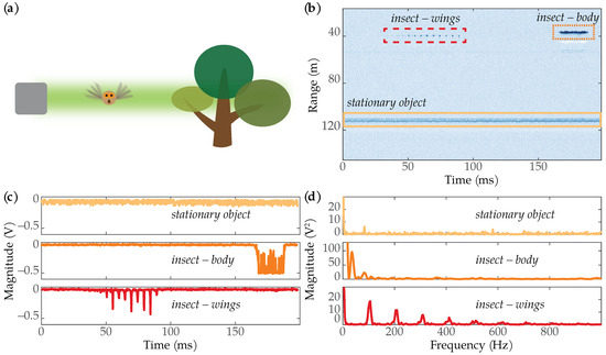
Figure 1.
(a) When an insect flies through the lidar beam and flaps its wings, the amount of reflected light changes. These changes in received intensity can be distinguished from other stationary objects. (b) An image showing a stationary object (yellow rectangle) and two insects: one where only the wings were in the lidar beam (dashed red rectangle), and one where the body of the insect was in the beam (dotted orange rectangle). The white-colored returns beneath the insects are reflections from the lidar’s wiring. (c) Time series plots showing the voltage magnitude of the three targets in (b). (d) Frequency spectra for each of the targets.
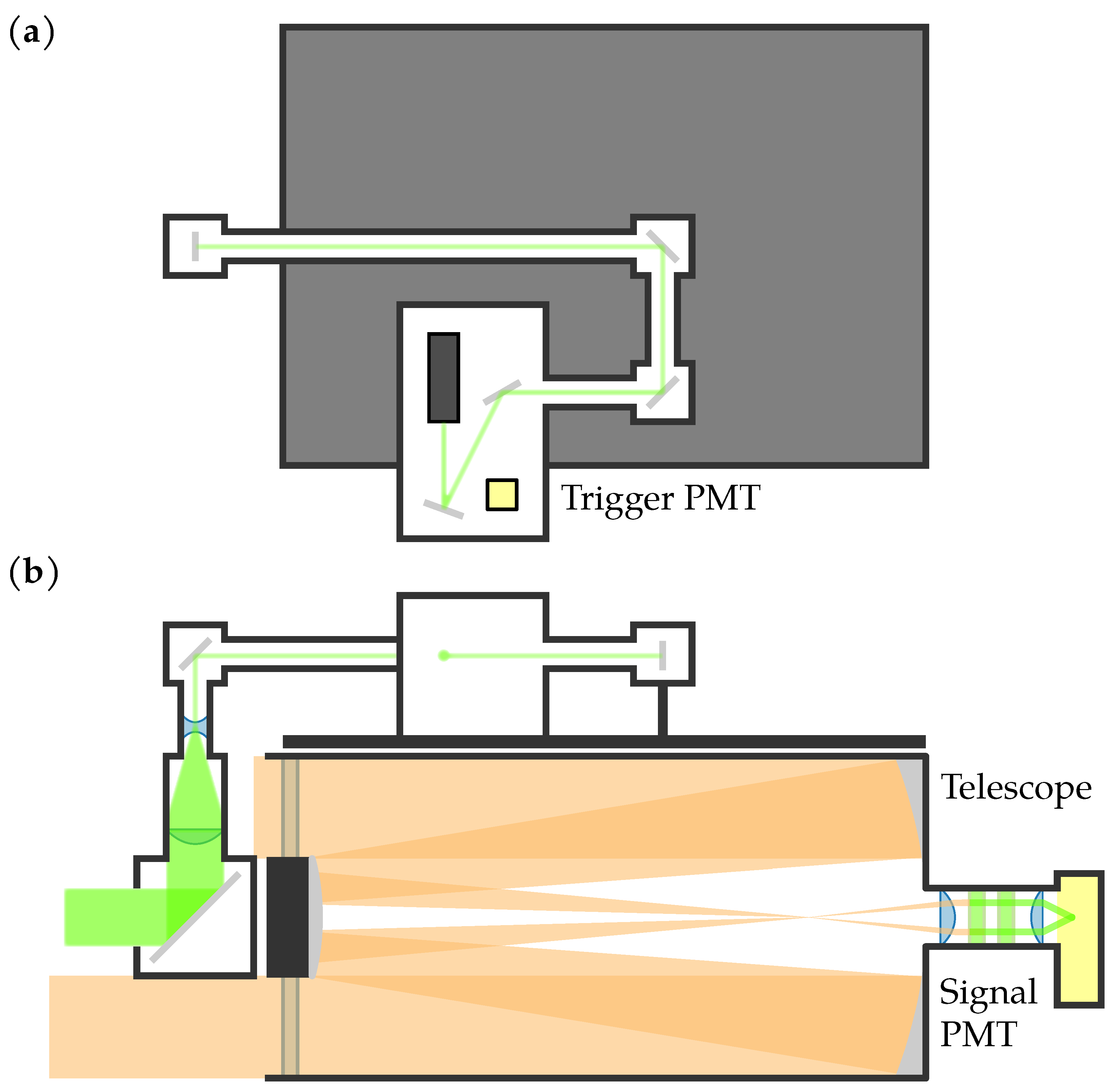
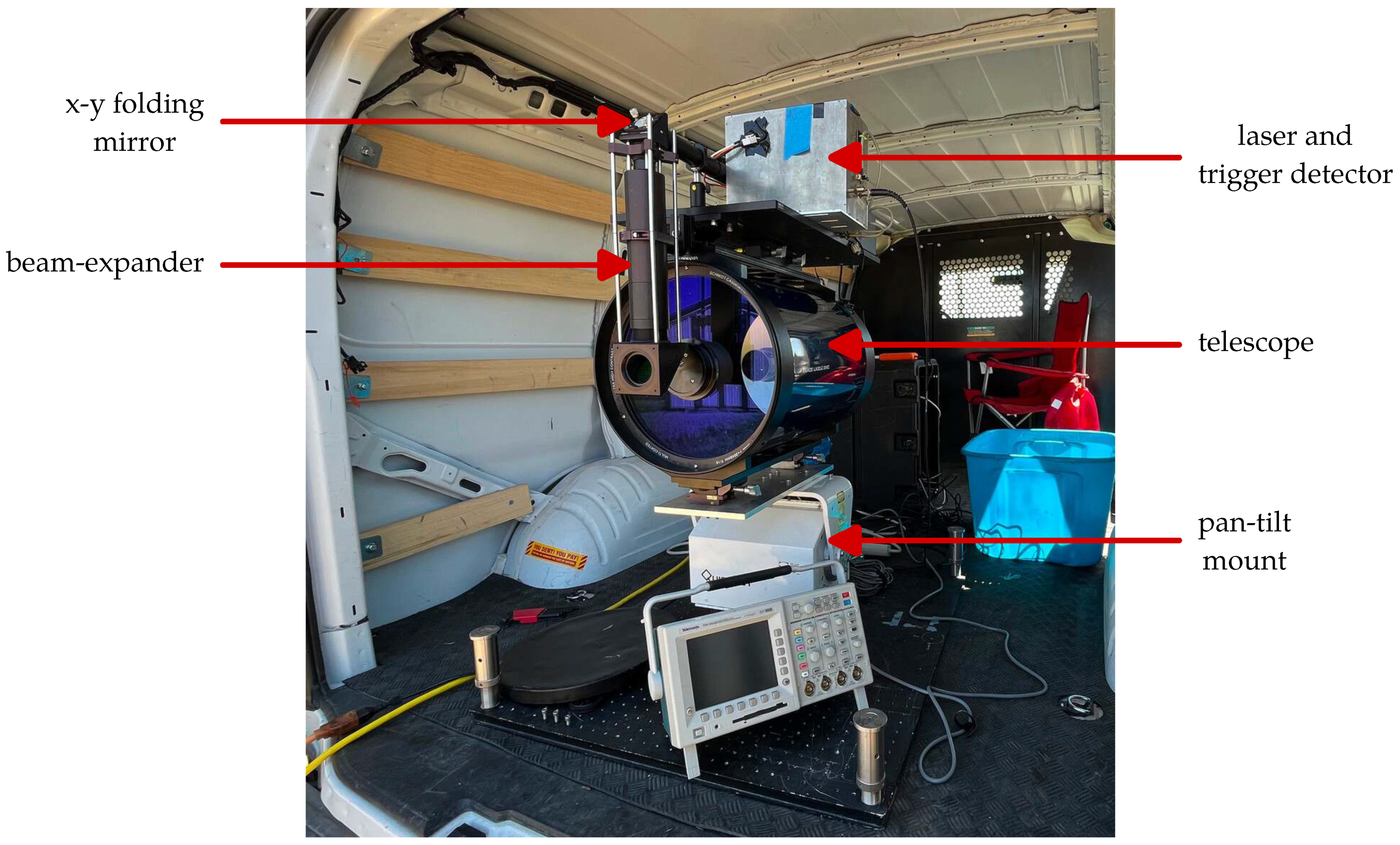
Figure 2 shows an optical schematic of the lidar system, and Figure 3 shows a picture of the lidar system during the experiments. The first component in the transmitting subsystem was the JDS Uniphase NG-10320-100 532 nm laser, which had a pulse width of 0.6 ns, a pulse energy of 3 , and a pulse repetition frequency (PRF) range between approximately 2.9 kHz to 5.4 kHz. The laser was housed in a light-tight box along with a Hamamatsu H6780-20 photomultiplier tube (PMT), the output of which was used as the trigger input for the analog-to-digital (ADC) converter. A series of mirrors and lens tubes directed the light out of the system at the center of the receiver telescope’s central obstruction. Before exiting the system, the beam was expanded to have a 50.8 mm diameter and half-angle divergence of 0.2 .
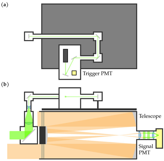
Figure 2.
Optical schematic of the lidar system. (a) Top view of the transmitting optics. (b) Side view of the transmitting and receiving optics. The PMTs are shown in yellow.
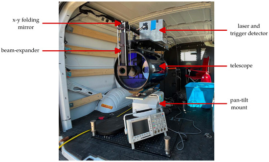
Figure 3.
Picture of the lidar system during data collection.
The first component in the receiving subsystem was the Meade LX200 Classic Schmidt-Cassegrain telescope with a 305 mm diameter and a focal length of 3048 mm. At the back of the telescope, a collimating lens, two laser line filters, and a focusing lens were housed in a lens tube. A Hamamatsu H9305-04 PMT was attached to the end of the lens tube. The lidar system was mounted on a MOOG QPT-130 pan-tilt mount.
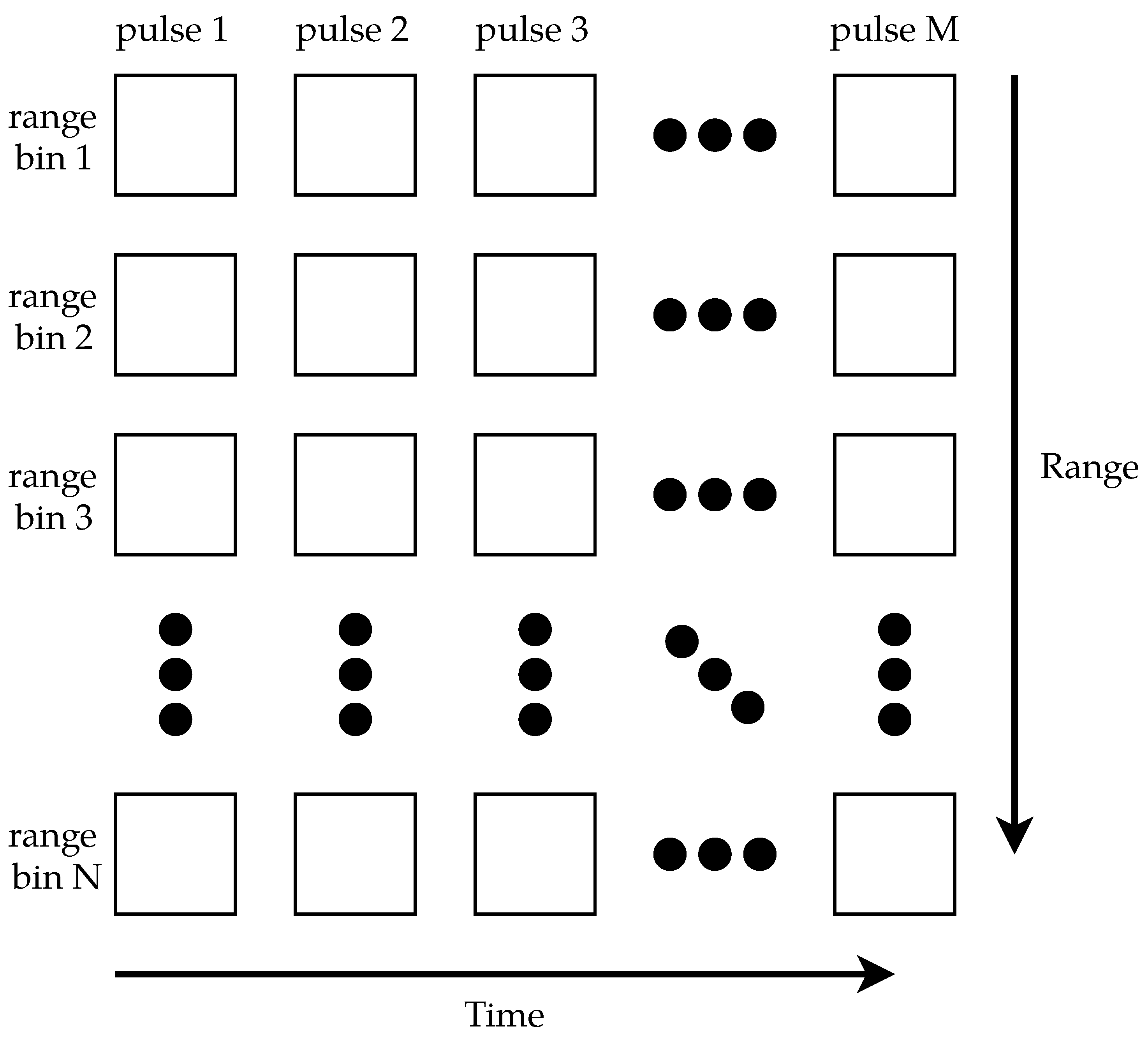
The data were digitized using a Compuscope 14200 PCIe ADC with a 200 / sampling rate, 100 MHz bandwidth, and 14-bit resolution. The 200 / sampling rate limited the system’s range resolution to 0.75 . The output of the H9305-04 PMT was connected to the ADC’s input channel, and the output of the H6780-20 PMT was connected to the ADC’s trigger input. For each laser pulse, the ADC was triggered to collect 200 samples. Due to the transit time for the light to leave the system, as well as variance in when the ADC started sampling, 178 samples were usable [49]. MATLAB was used to control the ADC and collect 1024 pulses, resulting in images of 178 rows (range bins) × 1024 columns (pulses). For compatibility with the ADC, MATLAB 2015b was used. Figure 4 shows a generic example of how the data were arranged into a matrix; the data are later visualized as false-color images. Since the laser’s PRF was not constant, the total duration of 1024 pulses was not constant; this resulted in images of varying durations.
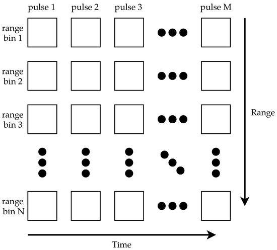
Figure 4.
A generic example of how the data were stored. Each column in the matrix represents one pulse of the lidar, and each row represents one range bin. Each matrix element is one sample.
2.2. Dataset
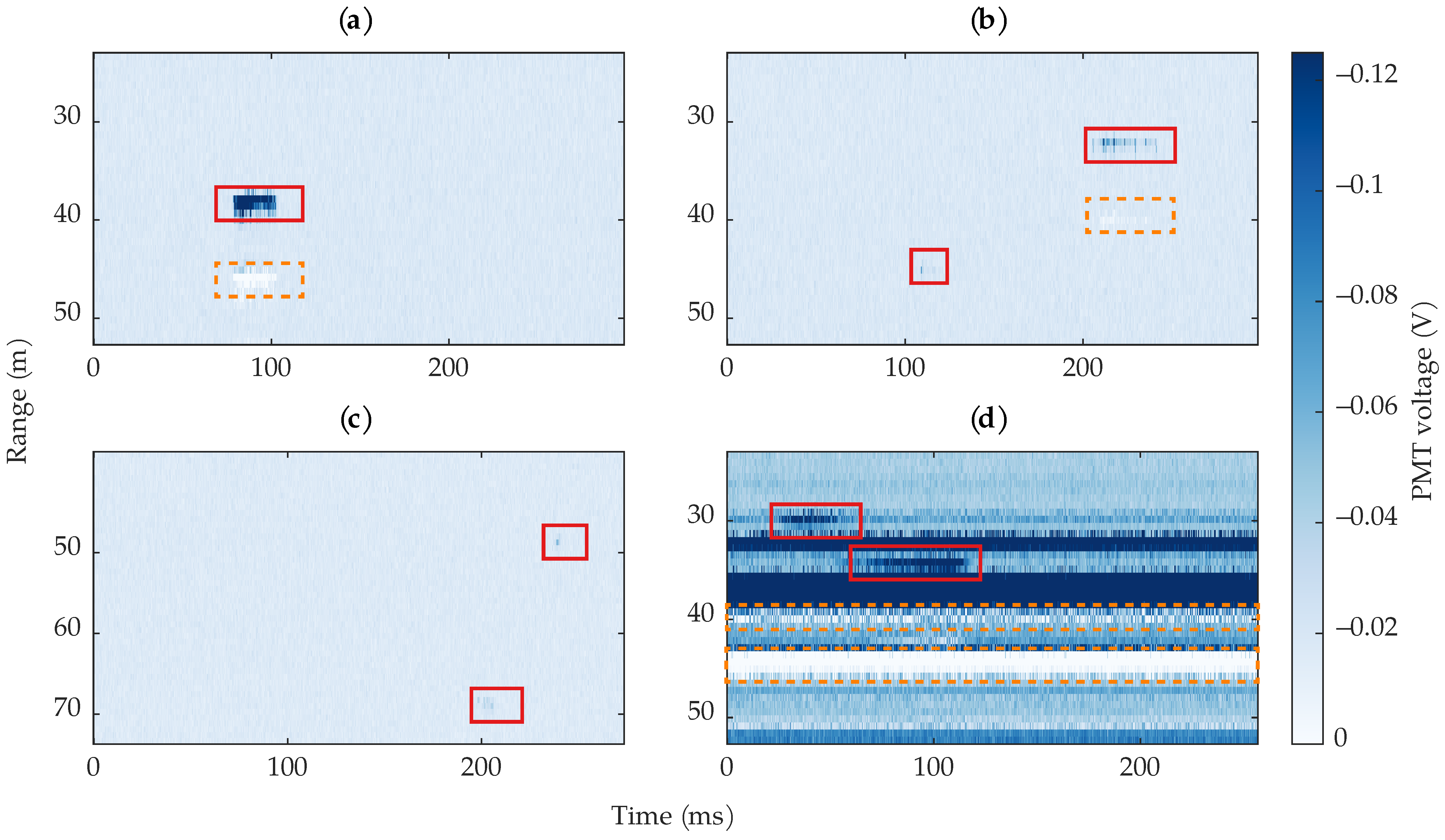
The data used for the experiments were collected in June and July 2022 at the MSU horticulture farm. The data comprise 9977 images taken in front of the beehives. As noted previously, the image durations vary because the laser’s PRF varied; this can be seen in Figure 5.

Figure 5.
Example images of different types of bees and images found in the dataset. For visualization clarity, the range of the images are cropped, and the colormap range is limited. The bees are surrounded by red rectangles; reflections are surrounded by orange dashed rectangles. (a) An example where the bee’s body dominated the return signal. (b) An example where the wing return dominated the signal (upper right rectangle), and an example of a very short-transit event (lower left rectangle). (c) Two examples of weak, short-transit observations. (d) An example of two long-transit signals where both the body and wing signals are present; the image also contains stationary, non-bee targets; the stationary objects have associated reflections, indicated by the orange dashed rectangles The duration of the four images are not the same due to the laser’s varying PRF.
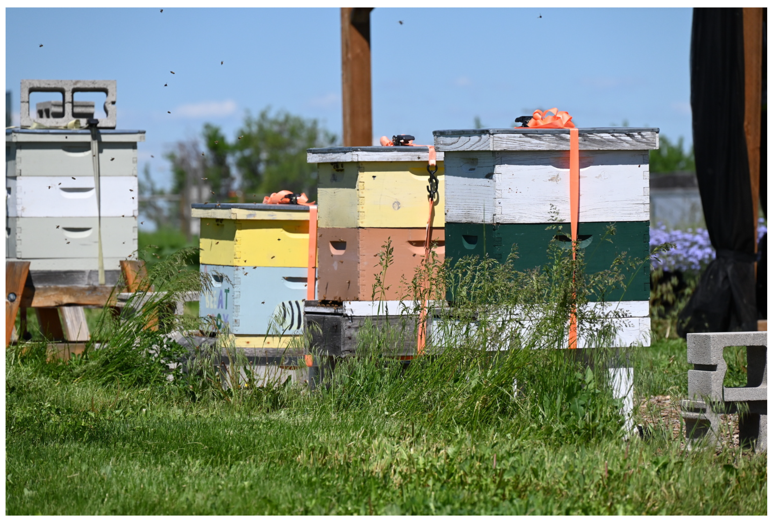
For the data collection process, the lidar was mounted in the back of a van, as shown in Figure 3, and pointed in front of the beehives, some of which are shown in Figure 6. The data were collected with the lidar beam pointed in various discrete directions; at each position, multiple images were collected while the lidar’s position was fixed. This was done to create a diverse set of measurements to train the machine learning algorithms on; having various levels of bee activity and background clutter helps avoid overfitting. The position of the lidar beam was controlled by changing the pan and tilt angles of the pan-tilt mount that the lidar was mounted on. The probability of bees flying through the lidar’s beam was a function of the beam’s position, as well as the various factors that influence bee activity (temperature, time of day, etc.).

Figure 6.
A picture of bee activity around some of the beehives. Four out of twelve beehives are shown. Some foliage was present near the beehive entrances, which sometimes shows up as background clutter in the collected images.
After collecting the data, we manually labeled the bounding box of each insect in each image, then converted the bounding boxes into binary labels that indicate whether a row contains an insect. Each potential insect was labeled with a confidence rating between 1 and 4 because some bees were more obvious than others. In general, high confidence ratings were assigned to bee events, which have obvious harmonic structure and a prominent return amplitude in the time domain. Low confidence ratings were given to events with very short transit times, such as those shown in Figure 5c. During the labeling process, we found 4671 probable bees. All labeled bees, regardless of confidence rating, were included in the dataset; our insect-detection algorithms did not account for confidence ratings. Since we were not able to collect ground-truth data in the field, it is possible that our labels are imperfect: some insects might have been missed, and some non-insects might have been labeled as insects. Our ground truth labels are the primary source of uncertainty. Using imperfect labels during training and validation may result in false insect detections; on the contrary, classifiers may find insects that the ground truth labels missed. Section 4.1 and Section 4.3 provide additional discussion on the effect of imperfect labels.
Of the 9977 images, 3498 (35.14%) contain one or more bees. In total, the dataset has 1,775,906 rows, 11,492 (0.647%) of which contain an insect measurement. Due to sampling jitter in the ADC, most insects span multiple range bins, leading to an increase in the number of rows that were labeled as containing insects. The dataset has a large class imbalance, particularly when looking at how many rows contain insects. Large class imbalances can cause machine learning algorithms to ignore the minority class [50], which would result in not detecting most insects. Section 2.4.1 discusses the methods we used to alleviate class imbalance.
Figure 5 shows four example images from the dataset containing different types of bee activity and stationary objects. The bee signals vary depending on whether the laser primarily hit the body or the wings of the bee. There is a low chance that the lidar pulses only hit the body, but the return from the body often dominates the signal when the incidence angle is such that the more specular wing reflection is not large. There are also images containing small blips of a bee where the laser might have barely hit the bee for a few pulses. These blips were labeled as bees but with a low confidence. When the intensity of returned light was large, reflections showed up in the data, which resulted in positive voltages at later range bins, as indicated by the orange dashed boxes in Figure 5. These artifacts are undesirable because they have similar characteristics to the actual returns that caused them. After the data were collected, we discovered that the reflections were caused by an impedance mismatch in the lidar’s wiring. By the time we discovered this, we could not recollect the data. Section 2.3 discusses our method to reduce the reflection artifacts.
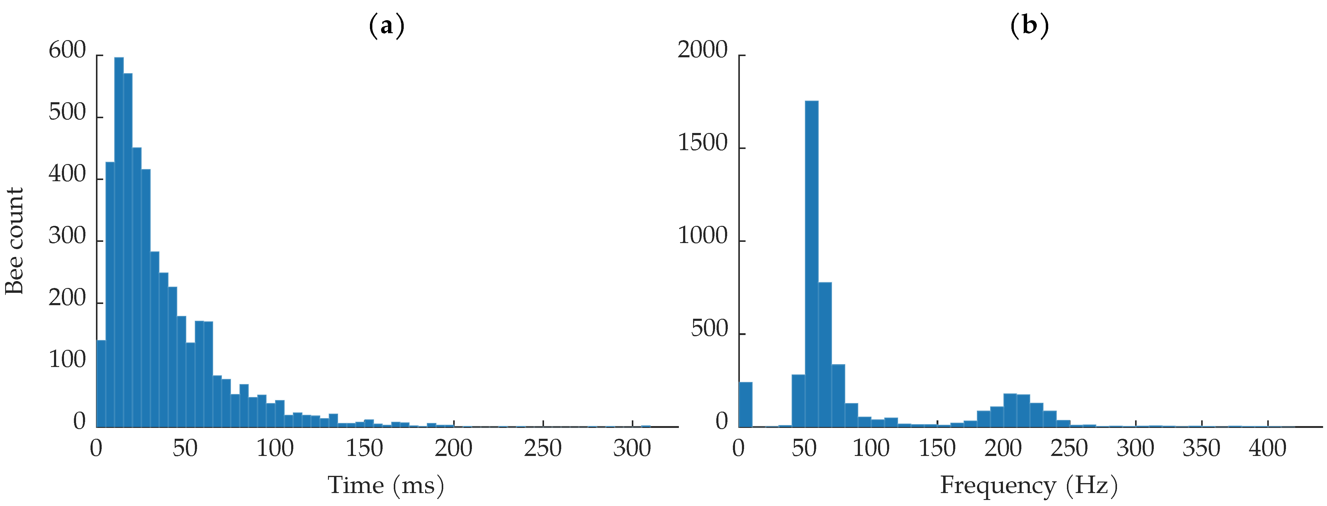
Figure 7a shows a histogram of the insect transit times observed in the dataset. The shortest transit time was 744 , the longest transit time was 307.9 , and the average transit time was 36.7 . Most bees were in the beam for less than 50 , which is about of the average image duration of 230 . Note that the image durations are not all the same. None of the recorded transit times can be longer than the associated image’s duration, though the object may have been in the beam for longer than the image’s duration. Nine events that were labeled as insects had transit times that lasted the entire image duration; most of these were labeled as low-confidence insects.

Figure 7.
(a) Histogram of bee transmit times. (b) Histogram of estimated fundamental wingbeat frequencies.
Figure 7b shows the distribution of fundamental wingbeat frequencies. Previous literature has found that honeybees’ fundamental wingbeat frequency can range from 150 to 600 and varies with environmental conditions [51]. The most common wingbeat frequencies are in the low 200 region [52,53]. The fundamental frequency of each insect observation was calculated using the harmonic product spectrum algorithm [54]. Since most insects showed up in multiple range bins due to sampling jitter, the fundamental frequency was estimated on the average of the insect’s range bins to increase the quality of the insect signals. Before estimating the fundamental frequency, the insect observations were bandpass filtered to help isolate the expected wingbeat frequencies. We used a 10th-order Butterworth filter with a passband between 50 and 1200 ; the upper passband frequency was chosen to ensure that the third harmonics in the spectra were left untouched, so as to not affect the harmonic product spectrum algorithm. The wingbeat frequency distribution shown in Figure 7b is distinctly bi-modal. In agreement with previous literature, we see a strong distribution of wingbeat frequencies between approximately 175 and 250 [51,52,53]. The other distribution of wingbeat frequencies, between 0 and approximately 125 , came from the bee observations where the body dominated the return signal and very little wingbeat motion was captured.
The data from June were used for training and validation, and the data from July were used for testing. This split simulates the scenario of training algorithms after one field campaign and then using the algorithms during the next campaign. The June data were split into stratified training and validation sets, with 80% for training and 20% for holdout validation. Table 1 shows the number of images, observations, and bees in each set.

Table 1.
Number of images, insect-containing images, rows, and insect-containing rows in the training, validation, and testing sets. The percentage of insect-containing images and insect-containing rows are shown in parentheses.
2.3. Preprocessing
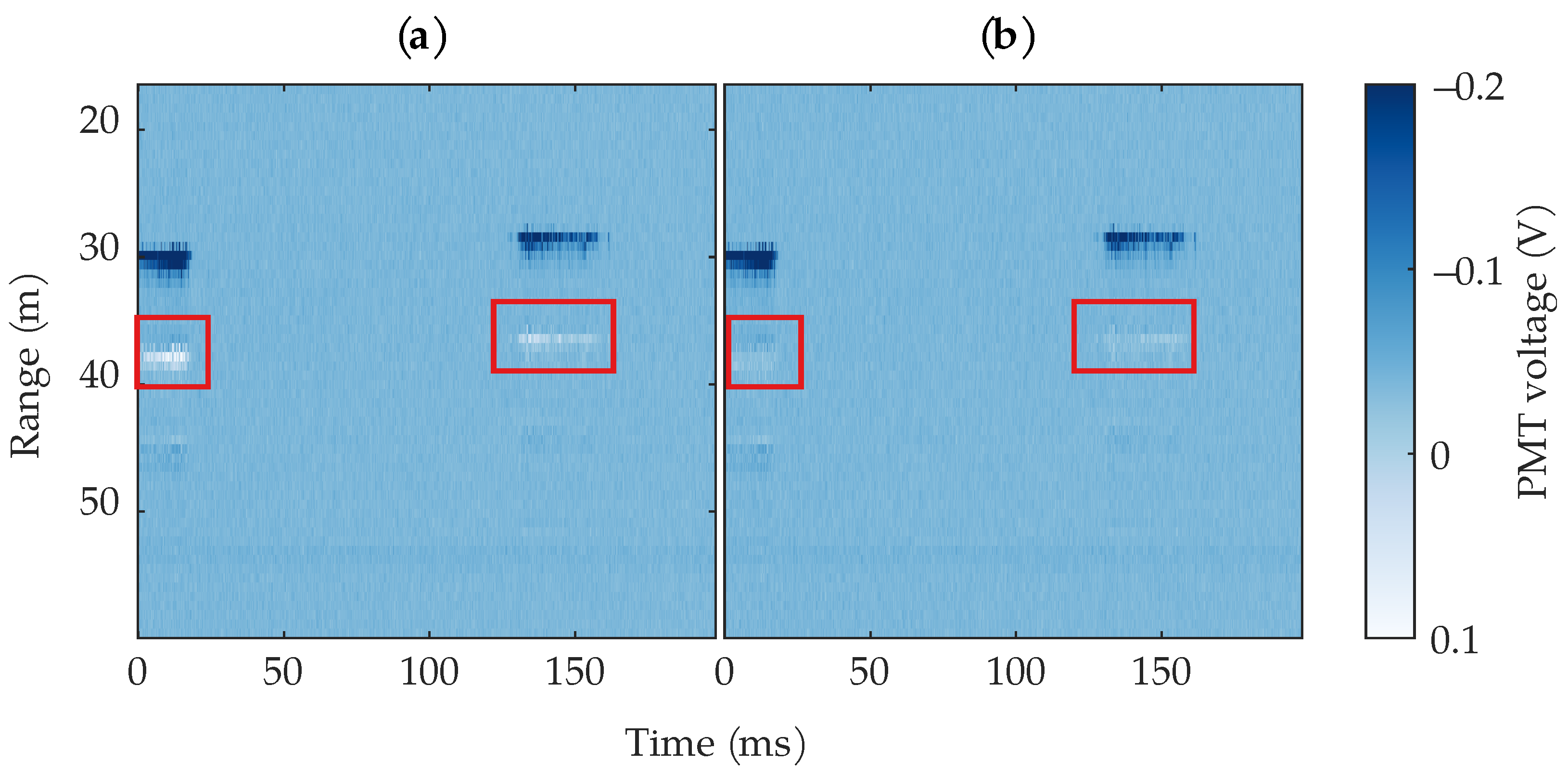
As mentioned in Section 2.2, an impedance mismatch caused reflections in the lidar’s wiring, which resulted in undesirable artifacts in the data. These artifacts can easily confuse the bee detection algorithms, as they share the same characteristics as the bee that produced them. Since the PMT output current is negative, any positive voltage values were due to reflections. Since the samples in each row form a time-series at a particular range bin, any large changes between subsequent samples would be caused by a moving object at that range bin. Using this knowledge, we thresholded all positive voltage values to the corresponding row’s average value. Figure 8 shows an example image before and after thresholding. The thresholding reduced most of the reflections, but not all, because some of the reflections resulted in small negative voltages near 0. Since we cannot easily distinguish between a small negative voltage caused by a reflection and a small negative voltage caused by a weak return from a bee or other object, we settle for leaving some artifacts in the data. While leaving these artifacts will increase the false positive rate of the algorithms, a more aggressive removal would result in missed insect detections.
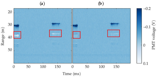
Figure 8.
Example of an image before (a) and after (b) thresholding the PMT ringing to the mean of the corresponding row. The ringing is highlighted by red rectangles. For visualization clarity, the range and colormap are limited.
2.4. Supervised Methods
The supervised learning methods we used can be broken into two categories: feature engineering and deep learning. The feature engineering methods use the features described in Section 2.4.2 as input, whereas the deep learning methods take the raw data as input. The methods can also be classified by whether they used rows as input or entire images as input. The feature engineering methods, as well as the 1-dimensional deep learning methods, predict which rows contain insects; the 2-dimensional deep learning methods take entire images as input and predict which images contain insects. For the row-based methods, the row predictions were aggregated to predict which images contain insects.
The overall supervised learning process comprised tuning dataset sampling parameters, tuning model hyperparameters, training, and testing. While our code attempts to make training as reproducible as possible by carefully seeding MATLAB’s random number generator, some algorithms were still not deterministic; consequently, we ran the whole process three times for each supervised learning algorithm.
2.4.1. Data Sampling
As mentioned previously, our dataset is highly imbalanced. To deal with this, we used combinations of data augmentation and random undersampling [50] while training the row-based methods. Data sampling was not performed for the image-based methods because the image-based dataset is not highly imbalanced.
Random undersampling was used to remove rows from each image that did not contain insects. To increase the number of insect examples used during training, we created synthetic insects. Our augmentation procedure performs 6 transformations: (1) random circular shifting; (2) interpolating the circularly-shifted vector; (3) decimating the circularly-shifted vector; (4) vector reversal; (5) interpolating the reversed vector; (6) and decimating the reversed vector. Random Gaussian noise is added to each synthetic observation. These transformations are performed in order. Consequently, when the number of synthetic observations, N, is not a multiple of 6, the last synthetic observations are created using the first n transformations from the list; for example, when the number of synthetic insects is 10, the last 4 synthetic insects are created using the first 4 transformations.
For the row-based methods, we performed a grid search over the following undersampling and data augmentation parameters:
- undersampling ratio:
- # of synthetic insects per insect observation:
During the grid search, the Matthew’s Correlation Coefficient (MCC) [55] was used to evaluate classification performance on the validation dataset. For each model, the sampling parameters with the highest MCC value were chosen as the final sampling parameters. During the grid search, the models were trained with their default hyperparameters.
2.4.2. Feature Engineering Methods
For the feature engineering methods, we trained four different types of models: AdaBoost [56], RUSBoost [57], a linear support vector machine (SVM), and multilayer perceptrons (MLP). AdaBoost and RUSBoost are both boosted decision tree ensembles, while the MLP is a feedforward neural network. We trained MLPs with 1, 3, 5, and 7 hidden layers.
The inputs to these models were 46 hand-selected features, which were extracted from each row in each image. From the time domain, we extracted the following features from each row: range, standard deviation, maximum absolute first difference, maximum absolute second difference, root-mean-square (RMS), impulse factor, crest factor, shape factor, median, median absolute deviation, mean-centered skewness, mean-centered kurtosis, and the observation mean minus the image mean. From the frequency domain, we extracted various statistics from the normalized one-sided energy spectral density (ESD): mean, median, median absolute deviation, standard deviation, mean-centered skewness, and mean-centered kurtosis. Most frequency-domain features were based upon the insect’s wingbeat frequency and harmonics, such as the height and location of each harmonic, as well as ratios of each harmonic’s features. The fundamental frequency was estimated from the normalized ESD using the harmonic product spectrum algorithm [54]. Before extracting any of the frequency domain features, the signals were bandpass filtered with a 10th order Butterworth filter with a passband between 50 and 1200 .
In addition to time- and frequency-domain features, we used generalized Morse wavelets [58] to compute the continuous wavelet scalogram, from which we extracted additional features. Across the time axis in the time-frequency plane, we computed the average intensity for each frequency bin, then selected the maximum of those intensity values. Similarly, we computed the standard deviation of each frequency bin and extracted the mean of those values. We also computed the maximum and mean values of the scalogram, the maximum change between adjacent values in the frequency axis, and the average skewness of the frequency bins. For a full list of features, see the feature ranking in Figure 9 and our code [59].
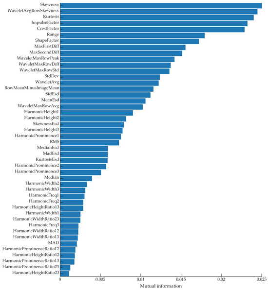
Figure 9.
A list of all features ranked by their mutual information with the class labels.
Individual model hyperparameters and the cost of predicting false negatives were tuned using Bayesian optimization [60], using MATLAB’s bayesopt function. Fifteen iterations were used during parameter tuning. MCC was again used to select the final hyperparameters. The search range for the false negative cost was integers between 1 and 10. For brevity, view our source code [59] for more information on the model-specific hyperparameter search ranges. The data sampling and model hyperparameter tuning were performed sequentially, rather than together. Our assumption was that the optimal data sampling parameters were independent of the individual model hyperparameters; although this assumption is likely not 100% true, performing the two tuning steps sequentially drastically reduces the parameter search space.
2.4.3. Deep Learning Methods
Given the rise of deep learning, we wanted to see if deep learning outperformed our manually engineered features. To this end, we tested two deep learning algorithms: a 2D convolutional neural network (CNN) that took the raw images as input, and a 1D CNN that operated on each row. For both CNNs, we tested models with 1, 3, 5, and 7 convolutional layers. Each convolution layer was followed by a batch normalization layer, a layer of rectified linear unit (ReLU) activation functions, and a dropout layer with a 20% dropout probability to reduce the chance of overfitting. Between the ReLU layer and the dropout layer, the 2D CNNs included a 2-by-2 max pooling layer with a stride of 2. Each model used weighted cross-entropy loss for the output layer. The default filter size for the 1D CNNs was 16, and the default filter size for the 2D CNNs was . A rectangular filter size was chosen as the default for the 2D CNNs because insect events are typically wider than they are tall.
All networks were trained using the Adam optimizer [61], though no efforts were made to optimize the training parameters; 20 training epochs and a learning rate of 0.01 were used for all models; the mini-batch size was 2048 and 64 for the 1D and 2D CNNs, respectively. The filter size, number of filters, and false negative cost for each model were tuned using the same procedure described in the previous section. For more architecture and training details, see our source code [59].
2.5. Changepoint Detection
The motivation for using changepoint algorithms was that bees show up as abrupt changes in both rows and columns. The experiments were conducted using MATLAB’s findchangepts function, a primarily statistical changepoint detection algorithm, and gfpop [62,63], a graph-based changepoint detection algorithm.
The findchangepts function is a part of MATLAB’s Signal Processing Toolbox and returns the index where the input signal changes most significantly. This algorithm utilizes a parametric global method of dividing the signal into two sections from some division point, calculating an estimate of the desired statistical property, measuring the deviation of the property at each point from the estimate, calculating total residual error, and then varying the division location until the total residual error is at its minimum. In this study, the mean was used as the statistical property. An experimentally determined minimum threshold of 0.0025 was used; this acts as a penalty value for the changepoint and sets the minimum improvement for the total residual error when calculating the changepoints.
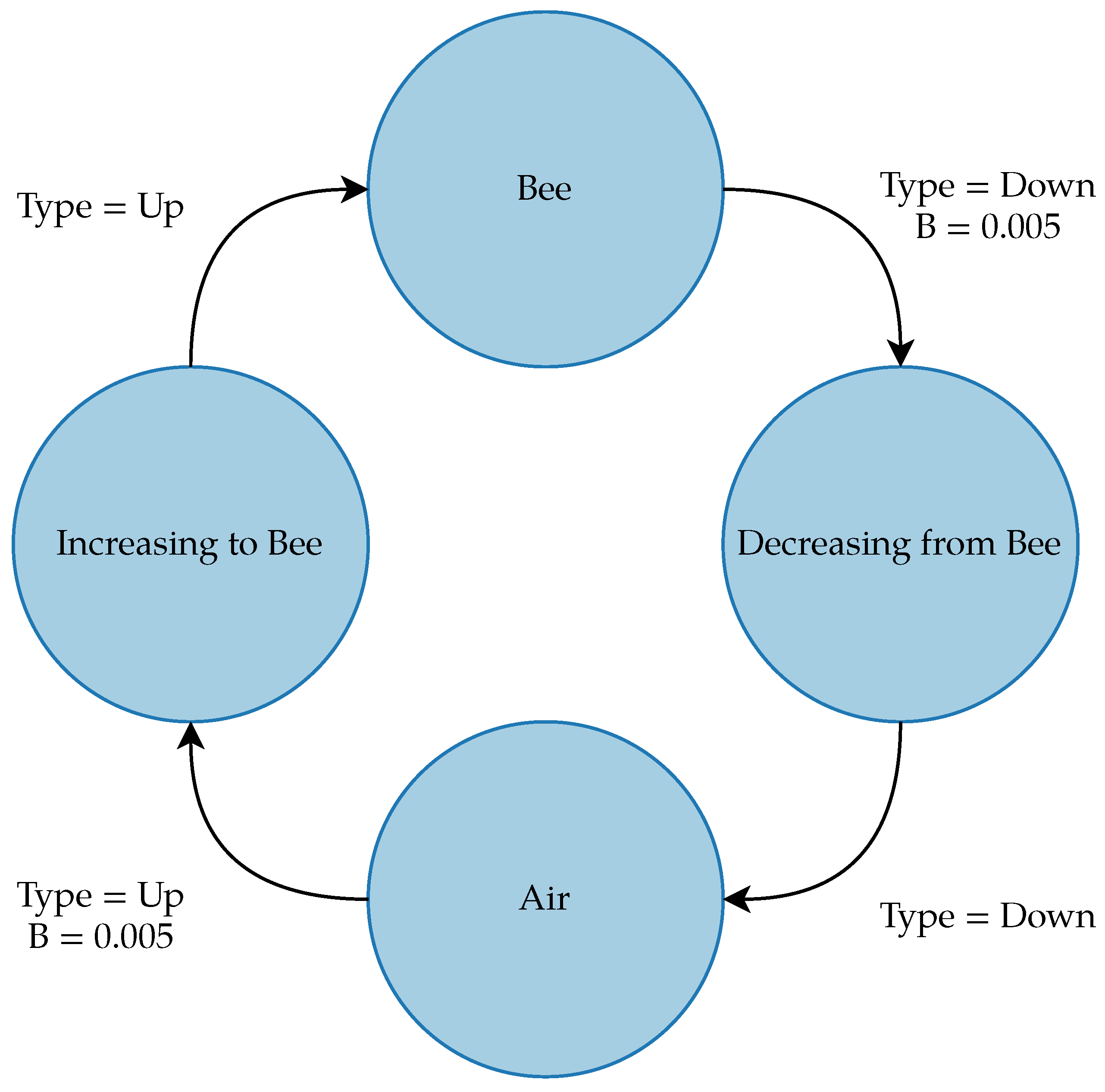
The gfpop (Graph Constrained Functional Pruning Optimal Partitioning) algorithm is a graph-based changepoint detection algorithm primarily created for applications in fields, such as medicine, containing large sequences of data with abrupt changes. The algorithm requires the user to input a built-in or manually created graph consisting of nodes representing the states of the signal, edges for the transitions between states, and a loss function to analyze the graph. The edges for the graph have a variety of parameters, although for this application, the only parameter that was tuned was the penalty on the edges for transitioning between states. The graph for the bee dataset, shown in Figure 10, contained four states representing air, bees, and the increase and decrease from the air to the bee; this graph gave better results than a binary graph of only air and bee states. The edges transitioning from the air to an increase and from the bee to a decrease had a penalty of 0.005. The graph penalties, as well as the procedures described below, were manually tuned on a few images from the training dataset.
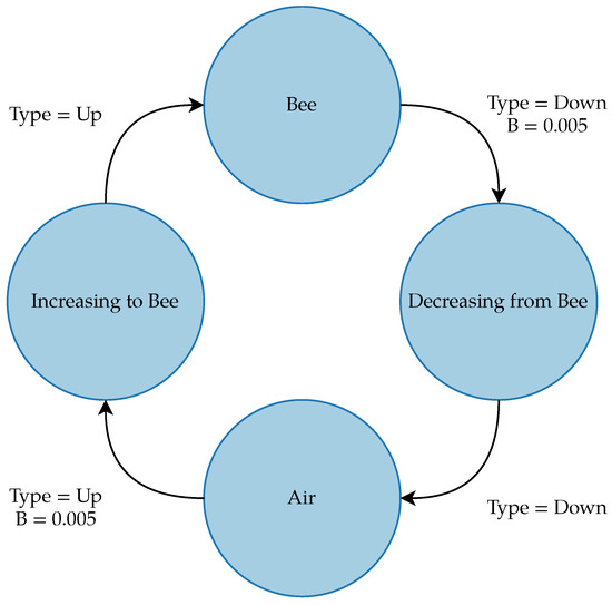
Figure 10.
gfpop graph for detecting bees in the dataset. Null edges that allow the algorithm to stay in the same state from point to point are not shown.
For the image analysis using the changepoint detection algorithms, both the rows and columns of the bee images were fed into the algorithms. The results were gathered based off of analyzing only the rows, only the columns, and checking both the rows and columns to see if they gave a changepoint within some margin.
The procedure for analyzing rows comprises the following steps: applying a heuristic to filter out rows that obviously do not contain bees, applying the changepoint detection algorithm to the remaining rows, then applying further heuristics to determine if the changepoints were likely associated with a bee signal. Concretely, we first check whether the range of the row is higher than the mean of the row. This was meant to check whether the target row was either empty air or a stationary object, as the empty air has a low range and a low mean, while stationary objects generally have a low range and high mean; if the range is greater than the mean, the row is marked as potentially containing a bee. The changepoint algorithm is then applied to these marked rows. After the algorithm is applied to the rows, the number of changepoints is checked, and if it is more than 5, the row is thrown out. This is because the stationary objects that pass through the first check often contained upwards of 10 changepoints, while the true bees often only contained around 5. The last check verifies that the voltage of the changepoint is larger than the mean of the row. If it is, then the changepoint is classified as a valid bee.
The procedure for analyzing the columns is similar. First, the algorithm checks the range of each row and compares it to the mean; from those results, the algorithm creates a vector of the valid rows where an insect could be. It then iterates through each column and checks whether the changepoints it detects are in valid rows before checking the value of the changepoint against the mean of the row. If the changepoint fits the same criteria used in the row analysis process, it is classified as a valid bee.
The process for checking both rows and columns involves iterating through the rows in the same manner as before, but after detecting changepoints in a row, it then iterates through those columns, and after finding a changepoint in the column, checks the norm between the changepoint it detected in the row and the changepoint it detected in the column. If they are within a distance of 4, as calculated by the L2 norm, the changepoint is considered to be a bee.
2.6. Evaluation Metrics
All the methods used were analyzed based on their recall, precision, and (MCC) [55] scores. It is well known that accuracy is not an informative metric for imbalanced data [64]; thus, accuracy is not used in this paper. Recall is the percentage of the target class that the method was able to identify and ranges from 0 to 1. Precision is the percentage of true positives relative to the total number of positive identifications and ranges from 0 to 1. MCC is a metric that gives a high score if the method is able to achieve an accurate value in each of the four categories of the confusion matrix. The MCC ranges between −1 and +1. Positive values indicate a positive correlation between the predictions and the true labels, with +1 being perfect prediction. A value of 0 indicates that the prediction is no better than random predictions. Negative values indicate a negative correlation between the predictions and the true labels, with −1 indicating complete disagreement between the predictions and the true labels.
When evaluating our methods, we consider recall more important than precision because the focus was to identify as many of the bees as possible. However, a low precision is not entirely outweighed by a high recall: low precision means there were many false positives, which researchers would have to look through to validate whether bees were present or not. Thus, a balance of recall and precision is desirable; a high MCC score indicates a good balance of recall and precision. While the score could be used as a single metric that combines recall and precision, we chose to use MCC because it is invariant to which class is labeled “positive”, unlike [65].
3. Results
The work in this paper has two performance goals: find which images contain insects and find the rows (i.e., range bins) the insects are located in. Methods that correctly detect most insect-containing images could be used on future datasets to reduce the number of images humans have to look through to label the insects. Likewise, methods that correctly detect most insect-containing rows would reduce the labeling burden, as well as help automatically compute parameters of interest, such as the number of insects and their wingbeat frequencies. While we ultimately want to detect all insects, we also want to have a reasonably high precision so we do not have to look through many false positives. For the methods that take rows as input, row-based and image-based results are reported. For the 2D CNNs, only image-based results are reported. The following sections detail the classification performance of the feature engineering, deep learning, and changepoint detection methods, as well as an in-depth analysis of the features described in Section 2.4.2.
3.1. Supervised Methods
3.1.1. Feature Analysis
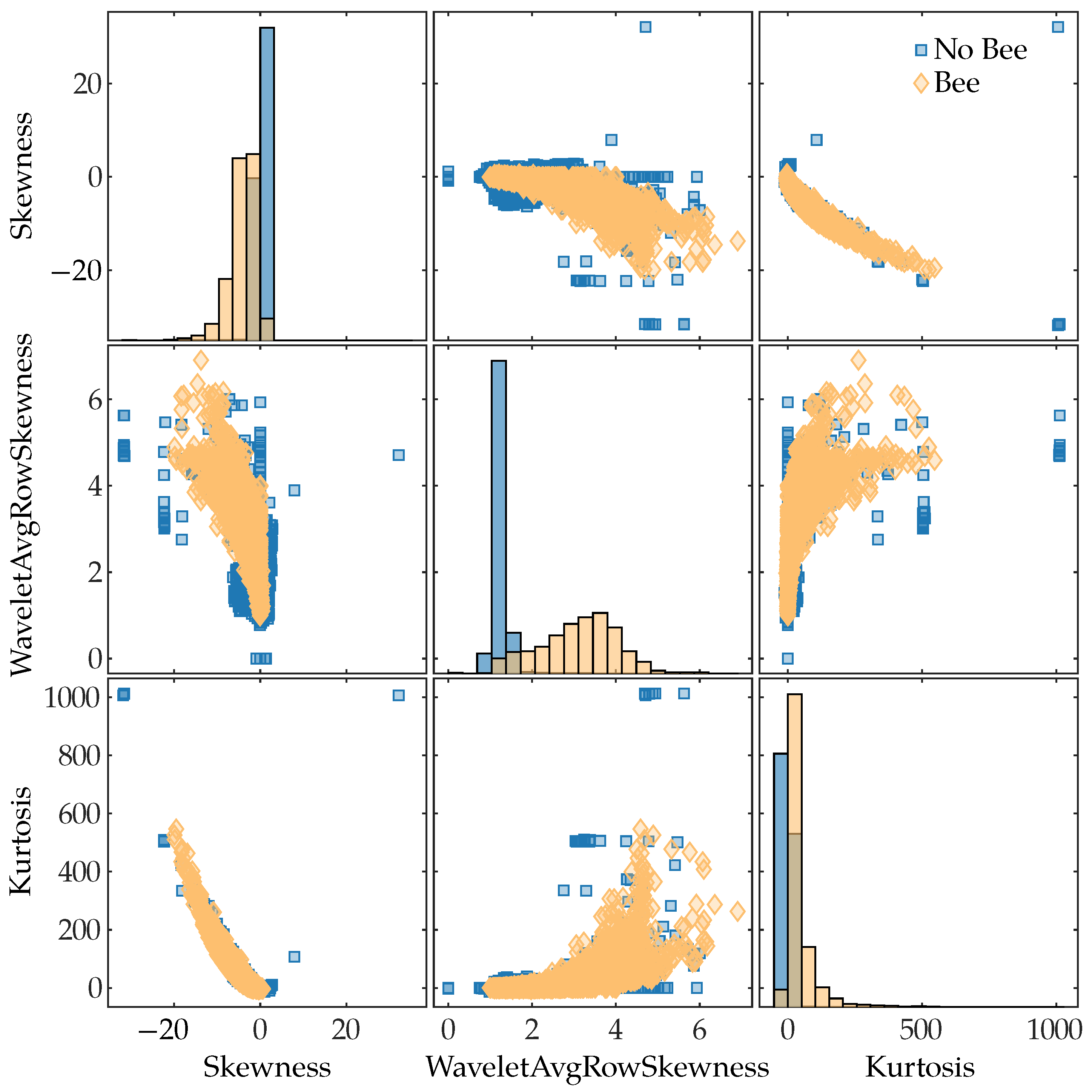
To see which of the extracted features had the most predictive power for discriminating between classes (“Bee” and “No bee”), we computed the mutual information [66] between the features and the class labels. We used the mutual_info_classif function from Python’s scikit-learn library to compute the mutual information scores; this function is based on a k-nearest-neighbor method of computing mutual information between continuous and discrete variables [67]. The results are shown in Figure 9. The top three features were the time-domain skewness, the average skewness of each row in the wavelet scalogram, and the time-domain kurtosis. Figure 11 shows a pairwise scatter plot of these three features; none of the top three features are separable, but there are clear differences between the “bee” and “no bee” distributions in Figure 11. The following paragraphs interpret the discrimination ability of each of the top three features.
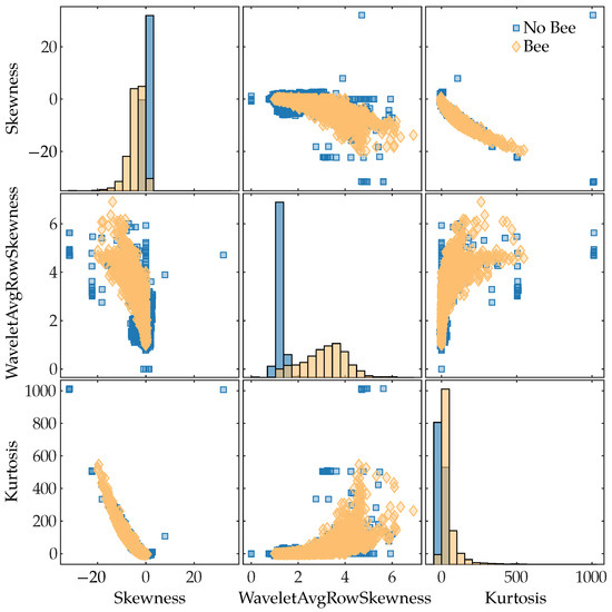
Figure 11.
Pairwise scatter plot of the three features with the highest mutual information with the class labels. The main diagonal shows histograms of each feature’s distribution. The features are ordered by descending mutual information values from top-to-bottom and left-to-right.
Skewness is a measure of asymmetry about the sample mean, with negative values indicating a long left tail of the distribution and positive values indicating a long right tail of the distribution. In our lidar data, insects flew through the beam for a small fraction of the total 1024 pulses; the pulses that hit insects have a large negative value compared to the rest of the pulses at that range bin, which results in a negative skewness. The majority of rows that do not contain insects have a skewness close to zero, as seen in Figure 11.
The rows of the wavelet scalogram correspond to frequency bins; thus, a row represents how a particular frequency component changes over time. Observations that did not contain any targets have little frequency content, which results in most of the scalogram values being close to 0; this leads to a small skewness value, as can be seen in “No Bee” distribution’s peak in the middle plot in Figure 11. When a bee is in the beam, its wings create frequency content in the return signal; this frequency content shows up in the relevant scalogram rows for a short period of time, which results in positive skewness for those rows. This is why the “Bee” distribution tends to have higher skewness values. However, there are also non-bee observations with high skewness, as seen in Figure 11.
Kurtosis is a measure of a distribution’s tail extremity; for the sample kurtosis, tail extremity indicates outliers in the data [68]. Rows that contain no targets are characterized by small amounts of noise and will have kurtosis values near 0, as seen by the peak in the “No bee” kurtosis distribution in Figure 11. Insects flying through the beam for short periods of time result in returns that differ significantly from their surroundings, i.e., they are outliers; consequently, insect rows will generally have a positive kurtosis value. Other noisy targets, such as moving blades of grass, will also tend to have positive kurtosis values.
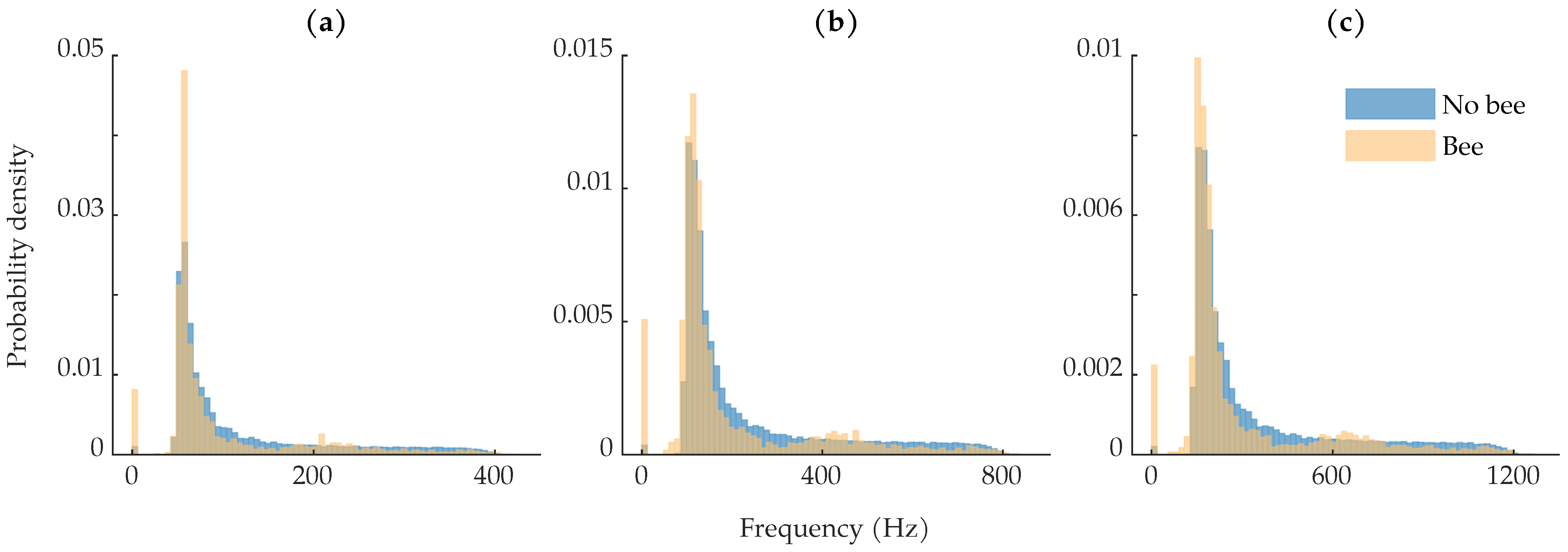
The low mutual information between the harmonic frequency values and the class labels, as seen in Figure 9, is surprising given that the wingbeat-modulation lidar method is based upon being able to determine the insects’ wingbeat spectra. This low mutual information is due to the significant overlap in the “Bee” and “No bee” harmonic frequency distributions, as shown in Figure 12. The distributions in Figure 12 were computed on each row of the training dataset. As seen in Figure 12a, compared to the “No bee” distribution, there is an extra bump in the “Bee” distribution around 200 , corresponding to the expected bee fundamental wingbeat frequency. The tails of the “No bee” distributions are more smooth, with no increase around the expected wingbeat frequencies. The majority of the “No bee” rows should exhibit no harmonic structure; in this case, an ideal frequency estimation algorithm would not report erroneous harmonic structure. Our fundamental frequency estimation algorithm looks for the largest local maximum in the harmonic product spectrum; if any local maxima exist, our algorithm returned an estimated frequency, otherwise the algorithm returned 0. In Figure 1d, the small peak around 100 in the stationary object’s spectrum would be interpreted as a local maxima and would thus be considered that observation’s fundamental frequency. This behavior is problematic for the non-bee observations and contributed to the overlap between the distributions.
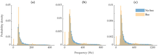
Figure 12.
Class-wise distributions of harmonic frequency computed on each row in the training set: (a) distribution of the first harmonic frequency; (b) distribution of the second harmonic frequency; (c) distribution of the third harmonic frequency. The counts at bin 0 are from observations where no local maximum was found in the harmonic product spectrum.
3.1.2. Data Sampling
Table 2 shows the undersampling and augmentation ratios that resulted in the best MCC scores on the validation set. The grid search was performed three times for each algorithm, and the results for each run are shown in Table 2. Most algorithms except the 1D CNNs did not benefit from data augmentation; this is partly in contrast to our previous work, where both AdaBoost and RUSBoost benefited from data augmentation [45]. Compared to our previous work, we have extracted more features, which might have helped the classifiers learn the decision boundary without data augmentation. There is no apparent pattern to which algorithms benefited from undersampling. Of the algorithms that selected different optimal undersampling ratios between the three runs, the associated MCC scores did not vary significantly, except for the SVM. However, MCC scores tended to vary significantly over the grid search parameters. As an example, one of the 5-layer 1D CNNs had MCC values range between 0.221 to 0.736. The data sampling results suggest that undersampling and oversampling can affect performance but that the optimal values are not necessarily independent of the model’s initial conditions, especially for the CNNs.

Table 2.
Undersampling and augmentation ratios that resulted in the best MCC scores on the validation set. The results are shown for each of the three runs.
3.1.3. Validation
For the row-based methods, the training set was sampled during hyperparameter tuning using the undersampling and augmentation ratios in Table 2; data sampling was not performed for the image-based methods. Table 3 shows the MCC scores that the tuned models obtained on the validation set after hyperparameter tuning. For the row-based methods, the best hyperparameters were chosen based upon the row-based MCC score. For all methods, if the default hyperparameters performed better than all hyperparameter combinations encountered during hyperparameter tuning, the default parameters were used for the final training.

Table 3.
Classification results on the validation set. The mean score from the three runs is shown, and the standard deviation is shown in parentheses. The best results for each metric are shown in bold. Methods marked with a * indicate that the method achieved the same results every run.
For the row-based methods, the feature-based MLPs obtained the best row-based average MCC scores on the validation set, as seen in Table 3. RUSBoost achieved the highest recall, at the expense of 45.3% precision. The 1D CNNs and the linear SVM all achieved average MCC scores around 0.75.
Looking at the image-based results in Table 3, we see that RUSBoost found the most insect-containing images, achieving the highest recall. The MLPs also performed well, achieving high precision scores above 93% and MCC values around 0.87. The three largest 2D CNNs achieved the top three average MCC scores, followed by the 3-layer MLP.
3.1.4. Testing
Using the best parameters found during the data sampling and hyperparameter tuning phases, each model was trained one final time on the full training and validation datasets. These trained models were then tested on the testing set, which was collected approximately one month after the training data was collected. Table 4 shows the recall, precision, and MCC scores that the models obtained on the testing set.

Table 4.
Classification results on the testing set. The mean score from the three runs is shown, and the standard deviation is shown in parentheses. The best results for each metric are shown in bold. Methods marked with a * indicate that the method achieved the same results every run.
For the row-based methods, RUSBoost performed the best, achieving a 0.948 recall and 0.752 MCC score. The majority of the methods did not generalize well to the training set, achieving significantly lower recall scores. However, the majority of the row-based methods performed well at identifying which images contained insects. This suggests that the methods were doing some combination of
- Finding the insects but not predicting all the rows that the insects spanned.
- Predicting insects in incorrect rows but doing so in images that contain insects.
- Missing some insects in images that contain multiple insects.
Looking at the image results in Table 4, we see that RUSBoost achieved the highest recall and MCC scores. The MLPs achieved the best MCC scores after RUSBoost. While the 1D CNNs often achieved high average recall, their recall and precision scores often varied significantly between the three runs, as indicated by the standard deviations in the image-based recall and precision columns. The 2D CNNs and AdaBoost did not generalize well to the testing set and achieved the lowest average recall and MCC scores.
Overall, RUSBoost achieved the best recall on both datasets and generalized to the testing set; this might be due in part to the undersampling RUSBoost performs during training, which creates a new undersampled dataset for each learner in the ensemble, rather than a single undersampled dataset for each learner. However, RUSBoost’s low precision, particularly on the validation set, is a potential downside; if one were to choose only one row-based model based on row-based validation-set performance, RUSBoost would not have been chosen. The feature-based MLPs performed consistently at detecting insect-containing images in both validation and testing sets; while their row-based testing results did not generalize as well, the consistent image-based performance is a plus for future applications. More discussion of model selection and algorithm recommendations follows in Section 4.
3.2. Changepoint Detection
The results for the changepoint detection algorithms were also gathered on both an image basis and a row basis using the testing set. For the image results shown in Table 5, when the two algorithms are compared, MATLAB’s findchangepts achieves a higher recall than gfpop. For the row results shown in Table 5, both algorithms struggled to achieve a high number of true positives; both algorithms achieved higher precision when analyzing the columns compared to analyzing the rows.

Table 5.
Changepoint detection results on the testing set. The best results for each metric are shown in bold.
One of the main motivations for using the changepoint detection algorithms was that the total runtime would be less than traditional machine learning algorithms, along with a decrease in required computational power. All the variations of the two algorithms were run with 32 CPUs and 80 GB of RAM. Since each image was independent of the other, the algorithms could process all the images in parallel before compiling the results together. The findchangepts function completed its workload in 21 s, 71 s, and 21 s for the rows, columns, and both, respectively. The gfpop algorithm completed its workload in 834 s, 1205 s, and 828 s for the rows, columns, and both, respectively. In general, these runtimes are far lower than the time it takes to train a machine learning algorithm.
Overall, the changepoint detection methods achieved lower row-based results than the supervised methods, on average. In particular, the changepoint detection methods achieved much lower row-based precision, indicating a higher number of false positives. This is due to the fact that any object that moves through the laser and has a significant return would result in a changepoint. The changepoint detection methods performed much better on the image-based metrics than on the row-based metrics, as seen in Table 5. While the changepoint detection methods still had worse image-based recall than RUSBoost, the gfpop rows and gfpop columns algorithms achieved the second and third best image-based recall, respectively. In spite of their comparable recall, the gfpop algorithms achieved lower image-based precision and MCC scores than the comparable supervised learning methods did; the MATLAB findchangepts “rows” and “both” methods, on the other hand, achieved precision comparable to many of the supervised methods. Since changepoint detection is an unsupervised method, the lower performance is not surprising: unsupervised methods do not have a priori knowledge of the class labels like supervised methods do and thus cannot be directly optimized to predict class labels [69]. Although the best supervised methods achieved better results, the changepoint methods achieved similarly high recall without needing to be trained on labeled data. This is a significant advantage for the changepoint detection methods, as labeling data is a time-consuming process.
4. Discussion
4.1. Sources of Uncertainty and Error
Our ground truth labels are the primary source of uncertainty. Since we manually labeled all insects via visual inspection, it is possible that some insects were missed and some non-insects were labeled as insects. Without any independent ground truth to validate our labels, we cannot easily verify that all labeled insects truly were insects; this is especially pertinent for observations that were labeled as low-confidence insects. The digitizer’s sampling jitter, which resulted in most insects spanning multiple 0.75 range bins during a single laser pulse (a physically impossible event), also contributed to uncertainty in the labels. When labeling each insect’s bounding box, deciding exactly how many rows the insect spanned was somewhat arbitrary because the effect of the sampling jitter decayed over multiple range bins. This decay and smearing can be seen in Figure 5.
4.2. Effects of Confidence Ratings
As noted in Section 2.2, the bee events were labeled with confidence ratings between 1 and 4, with 4 being the highest confidence rating. High-confidence bees had obvious signatures in both the time and frequency domains, whereas medium-confidence bees generally had obvious signatures in only one domain. For example, the two insect examples in Figure 1 are high-confidence bees, whereas the blips in Figure 5b,c are low-confidence bees. Thus, the confidence ratings are tied to labelling uncertainty and data quality. There are 73 rows with a confidence of 1, 1479 rows with a confidence of 2, 5288 rows with a confidence of 3, and 402 rows with a confidence of 4.
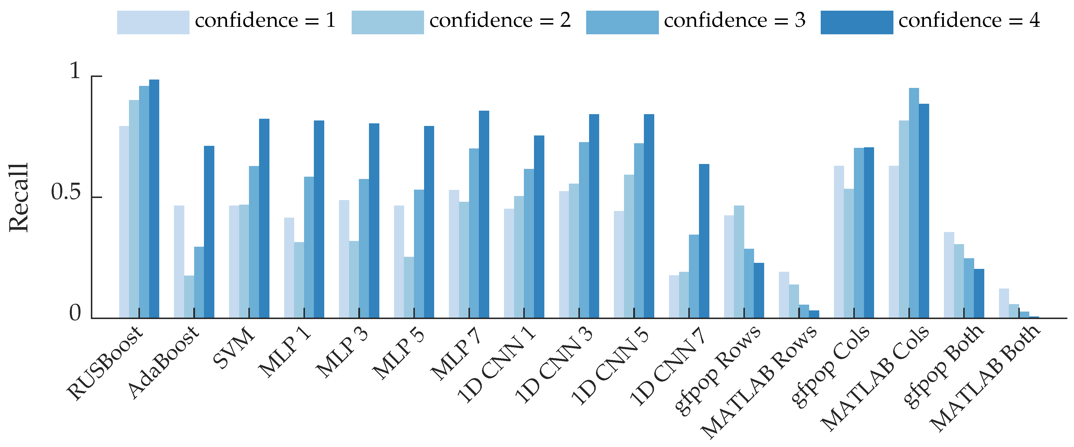
Figure 13 shows recall as a function of confidence rating. For the majority of the algorithms, the high-confidence bees are identified more often than low-confidence bees. This makes intuitive sense because high-confidence bees should be the most distinct. Interestingly, many of the supervised learning algorithms had higher recall for bees with a confidence of 1 than a confidence of 2. This suggests that the algorithms may have identified some salient features for low-confidence bees, such as the blips shown in Figure 5. These results could also be due to labeling uncertainty in the bounding boxes, as discussed in the following section, or imprecision of the confidence labels.

Figure 13.
Row-based recall grouped by the confidence ratings of the bee events. The average recall is displayed for the supervised learning algorithms.
Interestingly, the gfpop “rows” and MATLAB “rows” methods exhibit the opposite trend: recall decreases as confidence increases. The “both” methods exhibit the same trend because they are similar to the “rows” methods. It is possible that some of the high-confidence bee rows were discarded by the heuristic that bees typically had fewer than five changepoints. Conversely, low-confidence bees that were in the beam for a short period of time would have few changepoints and would thus pass through that heuristic. The column-based changepoint detection algorithms exhibit the expected behavior. High-confidence bees, especially ones which had a prominent body return signal, exhibit abrupt changes between range bins: range bins before and after the bee have a low return amplitude; this likely contributed to the behavior of the column-based changepoint methods shown in Figure 13.
4.3. Model Generalization
As noted in Section 3, many of the supervised methods did not perform as well on the testing set as they did on the validation set. This suggests some amount of overfitting to the training and validation sets, which were collected at a different time than the testing set. Although the training/validation and testing data were collected at the same location, the conditions were not exactly the same: ambient temperature was different, resulting in different bee activity; height of the foliage in front of the beehives was different; and some of the pan and tilt angles that the data were collected at were intentionally different. These variations resulted in different bee and background characteristics between the two datasets. Consequently, the training/validation and testing dataset distributions are not identical, nor are either of the sets representative of the entire possible data distribution at the data-collection location.
As was seen in Table 3 and Table 4, the methods generalized better when classifying images than classifying rows. This suggests that these methods were still detecting the insects but not detecting every row the insect occupied due to sampling jitter; or the methods simply missed an insect in images that contained multiple insects.
Figure 14a shows an example where a 3-layer MLP correctly found the insect but predicted more rows than were labeled. In this case, only one row was labeled but the insect spanned three rows, which the MLP predicted. This leads to an artificially low row-based precision, as the human labels were imperfect and did not span all the insect’s rows. Additionally, the MLP predicted the reflection artifacts as additional bees. Figure 14b shows the opposite case, where the 3-layer MLP predicted fewer rows than were labeled. Although the algorithm still found the bee, the missed rows led to an artificially low row-based recall. The situations demonstrated in Figure 14 show that the label ambiguity caused by the digitizer’s sampling jitter and the human-labeled bounding boxes contributed to artificially low row-based performance metrics.
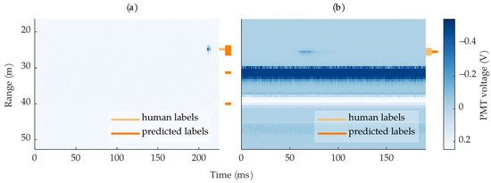
Figure 14.
Example images where a 3-layer MLP found the bee but did not achieve perfect recall or precision. (a) An example where the algorithm predicted extra rows compared to the human-labeled rows; the algorithm also predicted the ringing artifacts as bees. (b) An example where the algorithm predicted one out of three of the human-labeled rows.
Better generalization performance might have been achieved if we randomly split the combined June and July datasets into training/validation/testing sets, rather than using June for training/validation and July for testing. However, we wanted to model a real-world scenario where labeled data from a previous campaign could be used to train models for a new data collection campaign.
Overall, lack of generalization is one of the primary limitations of both the supervised and changepoint detection methods. It is unlikely that either category of methods will generalize to a new data-collection location or species without needing to be retrained or have some algorithm parameters adjusted. Additionally, recent insights have shown that CNNs with subsampled convolution and pooling operations are sensitive to small image translations [70]; it is possible that our 2D CNNs are sensitive to the bee locations, leading to lack of generalization, but some preliminary analysis suggests this is not the case. Eventually, as more data are collected across various locations, seasons, and species, the methods should start to generalize.
4.4. Algorithm Recommendations
For supervised learning, the general rule for model selection is to choose the model with the best validation performance. Based upon the row-based MCC, which was used during hyperparameter tuning, the 5-layer MLP would be chosen as the “best” model. Indeed, the 5-layer MLP also performed okay on the testing set, so this would not be a bad decision. However, RUSBoost, which had the lowest row-based MCC on the validation set, performed best on the testing set; RUSBoost did, however, have the highest row-based recall on the validation set, as well as the highest image-based recall on the validation set. Most methods’ generalization ability was better for the image-based results; given this, one might consider using the image-based validation results for final model selection, rather than the row-based results.
In general, for the supervised methods we tested, we recommend using RUSBoost and/or a feature-based MLP, as those methods performed consistently well across the validation and testing sets. The 1D CNNs achieved good average performance on the testing set but had high variability between runs; this variability indicates that the models were not robust. The 2D CNNs did not generalize to the testing set and also had high variability between runs. With more fine-tuned architectures, it is possible that CNNs could perform and generalize well.
Compared to the changepoint detection methods, the higher performance of the supervised methods comes at a cost: needing labeled data. Needing labeled data is the major limitation of the supervised methods because the primary point of automated detection is not having to manually detect insects. If labeled data already exist, then we recommend using one of the supervised methods. However, if labeled data does not exist, the changepoint detection methods are a promising place to start because they can be tuned on a few images and still achieved high recall of insect-containing images. If finding as many insect images as possible is paramount, and looking through false positives is not a huge burden, then we recommend the gfpop “rows” or “both” methods; these methods achieved image-based recall scores around 93%. If looking through many false positive images is too large of a burden, then we recommend the MATLAB “rows” or “both” algorithms because they achieved precision scores around 85%.
When the data are not labeled, a semi-supervised learning approach could be employed: use a changepoint detection method to create an initial set of imperfect labels, and then use those labels to train one of the supervised learning algorithms. The data could then be fed through the trained supervised algorithm, and any new positive predictions that were not predicted by the changepoint detection method can be inspected and labeled. This process can be repeated until no new insect images are found.
4.5. Future Research Directions
While good image-based recall and precision, like that achieved in this paper, would help reduce the amount of non-insect images requiring manual analysis, manual analysis would still need to be performed on the insect images to obtain quantities of entomological interest, such as the total number of insects observed. Consequently, future research should work towards improving the row-based insect detection performance and reducing sampling jitter; high row-based precision and recall would allow scientists to easily calculate the total number of insects, their spatial and temporal distributions, their wingbeat frequency distribution, etc. Towards this goal, the fundamental frequency estimation algorithm should be improved to detect less spurious harmonics in stationary object and noise observations. This would lead to better class separability in the harmonic features.
The sampling jitter is the biggest impediment to having an automatic count of the actual number of insects. The smearing of insect observations across multiple range bins limits the ability of the row-based methods to accurately detect insects and leads the row-based methods to produce artificially large insect counts. If the sampling jitter cannot be reduced significantly, post-processing methods should be explored. Using an image segmentation CNN is one possible solution, as the model could be trained to predict the insects’ bounding boxes.
Including the labels’ confidence ratings into the detection process is an interesting avenue for future work. The confidence ratings provide extra probability information that could prove useful. Lastly, we are also interested in trying more unsupervised and semi-supervised methods, such as anomaly detection methods.
5. Conclusions
Automatically detecting insects is crucial for the future of “big data” in entomology. In this paper, we present a comparison of supervised learning and changepoint detection methods for detecting insects using wingbeat-modulation lidar. We collected and published a new lidar dataset containing honeybee activity at various times and locations around a line of beehives. We found that both methods would be able to successfully reduce the need for manual data analysis: the supervised learning method with the best MCC score on the testing set correctly identified 99.5% of the insect-containing images and 83.7% of the non-insect images; the changepoint detection method with the best MCC score on the testing set correctly identified 83.2% of the insect-containing images and 84.2% of the non-insect images. In addition to comparing and recommending algorithms, we provide an analysis of which features were relevant for insect detection, which can help guide future development. Notably, we introduce wavelet-based features, which we have not seen in the previous literature; the wavelet-based features were all ranked in the top 50% of relevant features. While there is still room for improvement, the automated detection methods we present are capable of reducing the amount of manual data analysis required and can provide rough estimates of insect quantity and activity.
Author Contributions
Conceptualization, T.C.V., B.M.W. and J.A.S.; methodology, T.C.V., N.B.S., B.M.W. and J.A.S.; software, T.C.V. and N.B.S.; validation, T.C.V. and N.B.S.; formal analysis, T.C.V. and N.B.S.; investigation, T.C.V. and N.B.S.; resources, B.M.W. and J.A.S.; data curation, N.B.S. and T.C.V.; writing—original draft preparation, T.C.V. and N.B.S.; writing—review and editing, T.C.V., N.B.S., B.M.W. and J.A.S.; visualization, T.C.V., N.B.S. and J.A.S.; supervision, B.M.W., J.A.S. and T.C.V.; project administration, B.M.W.; funding acquisition, B.M.W. and J.A.S. All authors have read and agreed to the published version of the manuscript.
Funding
This material (AFRL-2023-5181) is based on research sponsored by Air Force Research Lab under agreement number FA8650-21-1-1176. The U.S. Government is authorized to reproduce and distribute reprints for Governmental purposes notwithstanding any copyright notation therein. The views and conclusions contained herein are those of the authors and should not be interpreted as necessarily representing the official policies or endorsements, either expressed or implied, of Air Force Research Lab or the U.S. Government.
Data Availability Statement
The data presented in this study are openly available on Zenodo at 10.5281/zenodo.10055762 (accessed on 30 October 2023), reference number [48].
Acknowledgments
Computational efforts were performed on the Tempest High Performance Computing System, operated and supported by University Information Technology Research Cyberinfrastructure at Montana State University. The authors would also like to acknowledge Caroline Xu and Ryan Ficken for performing prior work on changepoint detection and wavelet feature extraction, respectively. We would also like to acknowledge Caroline Xu, Ryan Ficken, and Walden Marshall for helping collect data. We thank the reviewers for their helpful comments that have improved this manuscript.
Conflicts of Interest
The authors declare no conflict of interest. The funders had a role in the decision to publish the results.
References
- McGavin, G.C. Essential Entomology: An Order-by-Order Introduction; Oxford University Press: Oxford, UK, 2001. [Google Scholar]
- Stork, N.E. How Many Species of Insects and Other Terrestrial Arthropods Are There on Earth? Annu. Rev. Entomol. 2018, 63, 31–45. [Google Scholar] [CrossRef] [PubMed]
- World Health Organization. Malaria Entomology and Vector Control; World Health Organization: Geneva, Switzerland, 2013. [Google Scholar]
- Mueller, U.G.; Gerardo, N.M.; Aanen, D.K.; Six, D.L.; Schultz, T.R. The Evolution of Agriculture in Insects. Annu. Rev. Ecol. Evol. Syst. 2005, 36, 563–595. [Google Scholar] [CrossRef]
- Wagner, D.L. Insect Declines in the Anthropocene. Annu. Rev. Entomol. 2020, 65, 457–480. [Google Scholar] [CrossRef] [PubMed]
- Outhwaite, C.L.; McCann, P.; Newbold, T. Agriculture and climate change are reshaping insect biodiversity worldwide. Nature 2022, 605, 97–102. [Google Scholar] [CrossRef] [PubMed]
- Cavender-Bares, J.; Schneider, F.D.; Santos, M.J.; Armstrong, A.; Carnaval, A.; Dahlin, K.M.; Fatoyinbo, L.; Hurtt, G.C.; Schimel, D.; Townsend, P.A.; et al. Integrating remote sensing with ecology and evolution to advance biodiversity conservation. Nat. Ecol. Evol. 2022, 6, 506–519. [Google Scholar] [CrossRef] [PubMed]
- McCravy, K. A Review of Sampling and Monitoring Methods for Beneficial Arthropods in Agroecosystems. Insects 2018, 9, 170. [Google Scholar] [CrossRef] [PubMed]
- Montgomery, G.A.; Dunn, R.R.; Fox, R.; Jongejans, E.; Leather, S.R.; Saunders, M.E.; Shortall, C.R.; Tingley, M.W.; Wagner, D.L. Is the insect apocalypse upon us? How to find out. Biol. Conserv. 2020, 241, 108327. [Google Scholar] [CrossRef]
- Eisen, L.; Eisen, R.J. Need for Improved Methods to Collect and Present Spatial Epidemiologic Data for Vectorborne Diseases. Emerg. Infect. Dis. 2007, 13, 1816–1820. [Google Scholar] [CrossRef]
- Høye, T.T.; Ärje, J.; Bjerge, K.; Hansen, O.L.P.; Iosifidis, A.; Leese, F.; Mann, H.M.R.; Meissner, K.; Melvad, C.; Raitoharju, J. Deep learning and computer vision will transform entomology. Proc. Natl. Acad. Sci. USA 2021, 118, e2002545117. [Google Scholar] [CrossRef]
- van Klink, R.; August, T.; Bas, Y.; Bodesheim, P.; Bonn, A.; Fossøy, F.; Høye, T.T.; Jongejans, E.; Menz, M.H.; Miraldo, A.; et al. Emerging technologies revolutionise insect ecology and monitoring. Trends Ecol. Evol. 2022, 37, 872–885. [Google Scholar] [CrossRef]
- Gibb, R.; Browning, E.; Glover-Kapfer, P.; Jones, K.E. Emerging opportunities and challenges for passive acoustics in ecological assessment and monitoring. Methods Ecol. Evol. 2018, 10, 169–185. [Google Scholar] [CrossRef]
- Drake, V.A.; Reynolds, D.R. (Eds.) Radar Entomology: Observing Insect Flight and Migration; CABI: Wallingford, UK, 2012. [Google Scholar] [CrossRef]
- Dwivedi, M.; Shadab, M.H.; Santosh, V.R. Insect Pest Detection, Migration and Monitoring Using Radar and LiDAR Systems. In Innovative Pest Management Approaches for the 21st Century; Springer: Singapore, 2020; pp. 61–76. [Google Scholar] [CrossRef]
- Noskov, A.; Bendix, J.; Friess, N. A Review of Insect Monitoring Approaches with Special Reference to Radar Techniques. Sensors 2021, 21, 1474. [Google Scholar] [CrossRef] [PubMed]
- Brydegaard, M.; Jansson, S. Advances in entomological laser radar. J. Eng. 2019, 2019, 7542–7545. [Google Scholar] [CrossRef]
- Tauc, M.J.; Fristrup, K.M.; Repasky, K.S.; Shaw, J.A. Field demonstration of a wing-beat modulation lidar for the 3D mapping of flying insects. OSA Contin. 2019, 2, 332. [Google Scholar] [CrossRef]
- Kouakou, B.K.; Jansson, S.; Brydegaard, M.; Zoueu, J.T. Entomological Scheimpflug lidar for estimating unique insect classes in-situ field test from Ivory Coast. OSA Contin. 2020, 3, 2362. [Google Scholar] [CrossRef]
- Rydhmer, K.; Prangsma, J.; Brydegaard, M.; Smith, H.G.; Kirkeby, C.; Schmidt, I.K.; Boelt, B. Scheimpflug lidar range profiling of bee activity patterns and spatial distributions. Anim. Biotelemetry 2022, 10, 14. [Google Scholar] [CrossRef]
- Wang, Y.; Zhao, C.; Dong, D.; Wang, K. Real-time monitoring of insects based on laser remote sensing. Ecol. Indic. 2023, 151, 110302. [Google Scholar] [CrossRef]
- Steenweg, R.; Hebblewhite, M.; Kays, R.; Ahumada, J.; Fisher, J.T.; Burton, C.; Townsend, S.E.; Carbone, C.; Rowcliffe, J.M.; Whittington, J.; et al. Scaling-up camera traps: Monitoring the planet’s biodiversity with networks of remote sensors. Front. Ecol. Environ. 2016, 15, 26–34. [Google Scholar] [CrossRef]
- Clayborn, J.; Clayborn, T. What happens in forests when nobody’s present? A sustainable method to document insect behaviors and interactions using video surveillance. Int. J. Trop. Insect Sci. 2019, 39, 341–345. [Google Scholar] [CrossRef]
- Preti, M.; Verheggen, F.; Angeli, S. Insect pest monitoring with camera-equipped traps: Strengths and limitations. J. Pest Sci. 2020, 94, 203–217. [Google Scholar] [CrossRef]
- Martineau, M.; Conte, D.; Raveaux, R.; Arnault, I.; Munier, D.; Venturini, G. A survey on image-based insect classification. Pattern Recognit. 2017, 65, 273–284. [Google Scholar] [CrossRef]
- Norouzzadeh, M.S.; Nguyen, A.; Kosmala, M.; Swanson, A.; Palmer, M.S.; Packer, C.; Clune, J. Automatically identifying, counting, and describing wild animals in camera-trap images with deep learning. Proc. Natl. Acad. Sci. USA 2018, 115, E5716–E5725. [Google Scholar] [CrossRef] [PubMed]
- Wäldchen, J.; Mäder, P. Machine learning for image based species identification. Methods Ecol. Evol. 2018, 9, 2216–2225. [Google Scholar] [CrossRef]
- Yousif, H.; Yuan, J.; Kays, R.; He, Z. Animal Scanner: Software for classifying humans, animals, and empty frames in camera trap images. Ecol. Evol. 2019, 9, 1578–1589. [Google Scholar] [CrossRef]
- Bjerge, K.; Nielsen, J.B.; Sepstrup, M.V.; Helsing-Nielsen, F.; Høye, T.T. An automated light trap to monitor moths (Lepidoptera) using computer vision-based tracking and deep learning. Sensors 2020, 21, 343. [Google Scholar] [CrossRef] [PubMed]
- Genoud, A.P.; Gao, Y.; Williams, G.M.; Thomas, B.P. A comparison of supervised machine learning algorithms for mosquito identification from backscattered optical signals. Ecol. Inform. 2020, 58, 101090. [Google Scholar] [CrossRef]
- Kirkeby, C.; Rydhmer, K.; Cook, S.M.; Strand, A.; Torrance, M.T.; Swain, J.L.; Prangsma, J.; Johnen, A.; Jensen, M.; Brydegaard, M.; et al. Advances in automatic identification of flying insects using optical sensors and machine learning. Sci. Rep. 2021, 11, 1555. [Google Scholar] [CrossRef]
- Bender, S.; Rodacy, P.; Schmitt, R.; Philip Hargis, J.; Johnson, M.; Klarkowski, J.; Magee, G.; Bender, G. Tracking Honey Bees Using LIDAR (Light Detection and Ranging) Technology; Technical Report; OSTI: Oak Ridge, TN, USA, 2003. [CrossRef]
- Shaw, J.A.; Seldomridge, N.L.; Dunkle, D.L.; Nugent, P.W.; Spangler, L.H.; Bromenshenk, J.J.; Henderson, C.B.; Churnside, J.H.; Wilson, J.J. Polarization lidar measurements of honey bees in flight for locating land mines. Opt. Express 2005, 13, 5853. [Google Scholar] [CrossRef]
- Hoffman, D.S.; Nehrir, A.R.; Repasky, K.S.; Shaw, J.A.; Carlsten, J.L. Range-resolved optical detection of honeybees by use of wing-beat modulation of scattered light for locating land mines. Appl. Opt. 2007, 46, 3007. [Google Scholar] [CrossRef]
- Shaw, J.A.; Repasky, K.S.; Carlsten, J.L.; Spangler, L.H.; Hoffman, D.S. Optical Detection of Oscillating Targets Using Modulation of Scattered Laser Light. U.S. Patent 7,511,624, 31 March 2009. [Google Scholar]
- Brydegaard, M.; Malmqvist, E.; Jansson, S.; Zhao, G.; Larsson, J.; Török, S. The Scheimpflug lidar method. In Proceedings of the Lidar Remote Sensing for Environmental Monitoring 2017, San Diego, CA, USA, 8–9 August 2017; Singh, U.N., Ed.; SPIE: Bellingham, WA, USA, 2017. [Google Scholar] [CrossRef]
- Guan, Z.; Brydegaard, M.; Lundin, P.; Wellenreuther, M.; Runemark, A.; Svensson, E.I.; Svanberg, S. Insect monitoring with fluorescence lidar techniques: Field experiments. Appl. Opt. 2010, 49, 5133. [Google Scholar] [CrossRef]
- Manefjord, H.; Muller, L.; Li, M.; Salvador, J.; Blomqvist, S.; Runemark, A.; Kirkeby, C.; Ignell, R.; Bood, J.; Brydegaard, M. 3D-Printed Fluorescence Hyperspectral Lidar for Monitoring Tagged Insects. IEEE J. Sel. Top. Quantum Electron. 2022, 28, 1–9. [Google Scholar] [CrossRef]
- Brydegaard, M.; Jansson, S.; Malmqvist, E.; Mlacha, Y.P.; Gebru, A.; Okumu, F.; Killeen, G.F.; Kirkeby, C. Lidar reveals activity anomaly of malaria vectors during pan-African eclipse. Sci. Adv. 2020, 6, eaay5487. [Google Scholar] [CrossRef] [PubMed]
- Jansson, S.; Malmqvist, E.; Mlacha, Y.; Ignell, R.; Okumu, F.; Killeen, G.; Kirkeby, C.; Brydegaard, M. Real-time dispersal of malaria vectors in rural Africa monitored with lidar. PLoS ONE 2021, 16, e0247803. [Google Scholar] [CrossRef] [PubMed]
- Malmqvist, E.; Jansson, S.; Torok, S.; Brydegaard, M. Effective Parameterization of Laser Radar Observations of Atmospheric Fauna. IEEE J. Sel. Top. Quantum Electron. 2016, 22, 327–334. [Google Scholar] [CrossRef]
- Rydhmer, K.; Bick, E.; Still, L.; Strand, A.; Luciano, R.; Helmreich, S.; Beck, B.D.; Grønne, C.; Malmros, L.; Poulsen, K.; et al. Automating insect monitoring using unsupervised near-infrared sensors. Sci. Rep. 2022, 12, 2603. [Google Scholar] [CrossRef]
- Rydhmer, K.; Selvan, R. Dynamic β-VAEs for quantifying biodiversity by clustering optically recorded insect signals. Ecol. Inform. 2021, 66, 101456. [Google Scholar] [CrossRef]
- Gebru, A.; Jansson, S.; Ignell, R.; Kirkeby, C.; Prangsma, J.C.; Brydegaard, M. Multiband modulation spectroscopy for the determination of sex and species of mosquitoes in flight. J. Biophoton. 2018, 11, e201800014. [Google Scholar] [CrossRef] [PubMed]
- Vannoy, T.C.; Scofield, T.P.; Shaw, J.A.; Logan, R.D.; Whitaker, B.M.; Rehbein, E.M. Detection of Insects in Class-Imbalanced Lidar Field Measurements. In Proceedings of the 2021 IEEE 31st International Workshop on Machine Learning for Signal Processing (MLSP), Gold Coast, Australia, 25–28 October 2021; IEEE: New York, NY, USA, 2021. [Google Scholar] [CrossRef]
- Sweeney, N.; Xu, C.; Shaw, J.A.; Hocking, T.D.; Whitaker, B.M. Insect Identification in Pulsed Lidar Images Using Changepoint Detection Algorithms. In Proceedings of the 2023 Intermountain Engineering, Technology and Computing (IETC), Provo, UT, USA, 12–13 May 2023; IEEE: New York, NY, USA, 2023. [Google Scholar] [CrossRef]
- LeCun, Y.; Bengio, Y.; Hinton, G. Deep learning. Nature 2015, 521, 436–444. [Google Scholar] [CrossRef]
- Vannoy, T.; Bradley, W. Dataset for Insect Detection Remote Sensing; Zenodo: Geneva, Switzerland, 2023. [Google Scholar] [CrossRef]
- Tauc, M. Scanning Wing-Beat-Modulation LIDAR for Insect Studies. Master’s Thesis, Montana State University, Bozeman, MT, USA, 2017. [Google Scholar]
- He, H.; Garcia, E.A. Learning from Imbalanced Data. IEEE Trans. Knowl. Data Eng. 2009, 21, 1263–1284. [Google Scholar] [CrossRef]
- Parmezan, A.R.S.; Souza, V.M.A.; Žliobaitė, I.; Batista, G.E.A.P.A. Changes in the wing-beat frequency of bees and wasps depending on environmental conditions: A study with optical sensors. Apidologie 2021, 52, 731–748. [Google Scholar] [CrossRef]
- Altshuler, D.L.; Dickson, W.B.; Vance, J.T.; Roberts, S.P.; Dickinson, M.H. Short-amplitude high-frequency wing strokes determine the aerodynamics of honeybee flight. Proc. Natl. Acad. Sci. USA 2005, 102, 18213–18218. [Google Scholar] [CrossRef] [PubMed]
- Vance, J.T.; Altshuler, D.L.; Dickson, W.B.; Dickinson, M.H.; Roberts, S.P. Hovering Flight in the Honeybee Apis mellifera: Kinematic Mechanisms for Varying Aerodynamic Forces. Physiol. Biochem. Zool. 2014, 87, 870–881. [Google Scholar] [CrossRef]
- Schroeder, M.R. Period Histogram and Product Spectrum: New Methods for Fundamental-Frequency Measurement. J. Acoust. Soc. Am. 1968, 43, 829–834. [Google Scholar] [CrossRef] [PubMed]
- Matthews, B.W. Comparison of the predicted and observed secondary structure of T4 phage lysozyme. Biochim. Biophys. Acta (BBA)-Protein Struct. 1975, 405, 442–451. [Google Scholar] [CrossRef]
- Freund, Y.; Schapire, R.E. Experiments with a new boosting algorithm. In Proceedings of the ICML, Bari, Italy, 3–6 July 1996; Citeseer: University Park, PA, USA, 1996; Volume 96, pp. 148–156. [Google Scholar]
- Seiffert, C.; Khoshgoftaar, T.M.; Hulse, J.V.; Napolitano, A. RUSBoost: A Hybrid Approach to Alleviating Class Imbalance. IEEE Trans. Syst. Man Cybern. Part A Syst. Hum. 2010, 40, 185–197. [Google Scholar] [CrossRef]
- Olhede, S.; Walden, A. Generalized Morse wavelets. IEEE Trans. Signal Process. 2002, 50, 2661–2670. [Google Scholar] [CrossRef]
- Vannoy, T.; Sweeney, N.; Whitaker, B. BMW-Lab-MSU/Insect-Detection-Remote-Sensing-mdpi: v1.0.0; Zenodo: Geneva, Switzerland, 2023. [Google Scholar] [CrossRef]
- Maurya, A. Bayesian optimization for predicting rare internal failures in manufacturing processes. In Proceedings of the 2016 IEEE International Conference on Big Data (Big Data), Washington, DC, USA, 5–8 December 2016; IEEE: New York, NY, USA, 2016. [Google Scholar] [CrossRef]
- Kingma, D.P.; Ba, J. Adam: A Method for Stochastic Optimization. arXiv 2014, arXiv:1412.6980. [Google Scholar]
- Runge, V.; Hocking, T.D.; Romano, G.; Afghah, F.; Fearnhead, P.; Rigaill, G. gfpop: An R Package for Univariate Graph-Constrained Change-Point Detection. arXiv 2020, arXiv:2002.03646. [Google Scholar] [CrossRef]
- Hocking, T.D.; Rigaill, G.; Fearnhead, P.; Bourque, G. Constrained Dynamic Programming and Supervised Penalty Learning Algorithms for Peak Detection in Genomic Data. J. Mach. Learn. Res. 2020, 21, 1–40. [Google Scholar]
- Weiss, G.M. Mining with rarity. ACM SIGKDD Explor. Newsl. 2004, 6, 7–19. [Google Scholar] [CrossRef]
- Chicco, D.; Jurman, G. The advantages of the Matthews correlation coefficient (MCC) over F1 score and accuracy in binary classification evaluation. BMC Genom. 2020, 21, 6. [Google Scholar] [CrossRef] [PubMed]
- Cover, T.M. Elements of Information Theory; John Wiley & Sons: Hoboken, NJ, USA, 1999. [Google Scholar]
- Ross, B.C. Mutual Information between Discrete and Continuous Data Sets. PLoS ONE 2014, 9, e87357. [Google Scholar] [CrossRef] [PubMed]
- Westfall, P.H. Kurtosis as Peakedness, 1905–2014. R.I.P. Am. Stat. 2014, 68, 191–195. [Google Scholar] [CrossRef] [PubMed]
- Hastie, T.; Tibshirani, R.; Friedman, J. The Elements of Statistical Learning: Data Mining, Inference, and Prediction, 2nd ed.; Springer Nature: Berlin, Germany, 2009; Chapter 14.1. [Google Scholar]
- Azulay, A.; Weiss, Y. Why do deep convolutional networks generalize so poorly to small image transformations? JMLR 2019, 20, 1–25. [Google Scholar] [CrossRef]
Disclaimer/Publisher’s Note: The statements, opinions and data contained in all publications are solely those of the individual author(s) and contributor(s) and not of MDPI and/or the editor(s). MDPI and/or the editor(s) disclaim responsibility for any injury to people or property resulting from any ideas, methods, instructions or products referred to in the content. |
© 2023 by the authors. Licensee MDPI, Basel, Switzerland. This article is an open access article distributed under the terms and conditions of the Creative Commons Attribution (CC BY) license (https://creativecommons.org/licenses/by/4.0/).


