Dynamic Analysis of a Long Run-Out Rockslide Considering Dynamic Fragmentation Behavior in Jichang Town: Insights from the Three-Dimensional Coupled Finite-Discrete Element Method

Abstract

To clearly realize the dynamic process as well as the dynamic fragmentation behavior of a long run-out rockslide, a novel numerical method for landslide simulation of the coupled finite-discrete element method (FDEM) was applied and the Jichang rockslide was used as a case. The calibrated simulation result of the FDEM in a rockslide deposit corresponds well with the real rockslide deposit. The main run-out process of the rockslide lasts for 75 s and can be divided into acceleration and deceleration stages, which last for 33 s and 42 s, respectively. The maximum overall rockslide movement speed is 35 m/s while the partial sliding mass reaches 45 m/s. The fracturing, fragmentation, and disintegration processes of the sliding mass can be clearly observed from the dynamic scenarios. Fracture energy generated by rock fracturing constantly increases with time in a non-linear form. Of the total fracture energy, 54% is released in the initial 5 s because of fracturing, and 39% of the total fracture energy is released because of fragmentation and disintegration in the last 35 s. The accumulated friction energy increases in the whole run-out process, and its magnitude is much greater than the kinetic energy and fracture energy of the sliding mass.

1. Introduction

Long run-out rockslides are one of the most common and catastrophic geological disasters in nature. In the major high mountainous areas all over the world, long run-out rockslides are widely distributed [1,2,3,4,5,6,7,8,9]; they have an excessively high movement speed and a large affected area compared to normal landslides because of dynamic fragmentation [10]. However, their run-out processes are rare to be observed directly because of their suddenness and invisibility. Meanwhile, the dynamic process of rock material is difficult to study quantitively. Knowing their dynamic process considering dynamic fragmentation is very important and benefits the further study of the movement mechanism of their long run-out behavior.

Numerical simulation can reflect landslide movement scenarios and kinematic quantitative parameters directly. It has become the most important way to study landslide dynamic process in recent years [11,12,13]. There are several numerical methods that have been applied to landslide simulation, including the discontinuum methods of discontinuous deformation analysis (DDA) [14,15] and the discrete element method (DEM) [16], as well as the continuum methods of the depth-integrated model (DIM) [17,18], material point method (MPM) [19,20], and smoothed particle hydrodynamics (SPH) [21,22,23,24]. The continuum methods describe landslide movement behavior by macroscopic stress–strain constitutive equations or flow governing equations. The discontinuum methods use a group of independent discrete elements representing sliding mass. Interaction between these independent discrete elements as well as their movement constitutes macroscopic movement behavior of the sliding mass. Compared to the discontinuum methods, the continuum methods have the potential to integrate more kinds of governing equations for different conditions but they still have some limitations in simulating fracturing, fragmentation, and separation behaviors. This makes the continuum methods more suitable to simulate continuous flow behavior such as the debris flow but cannot completely reflect a rockslide movement process because a rockslide includes the fragmentation and disintegration processes of a source material [25,26]. In the rockslide simulations, the particle flow code (PFC) model plays the most important role and is the most widely applied for its stability and high computational efficiency. However, there are still some limitations for PFC to simulate a rockslide. First, the real source rock is frequently compacted macroscopically. However, there are many pores existing in the source rock in the PFC model due to a limited number of spheres composing the source rock. It makes the structure of the simulated source rock different from the real source rock. Second, fractures exist in the form of surfaces in the real source rock, but fractures in the PFC model based on the bonded particle model (BPM), which are most frequently used to simulate a rockslide, are based on point-to-point contact, making the present form of fracture different from the real rock.

To overcome the above limitations of the PFC model in rockslide simulation, the finite-discrete element method (FDEM) was applied to simulate a rockslide in this manuscript. The FDEM is a method developed from a sketch of the finite element methods; a type of cohesive interface element (CIE) is inserted into the boundaries of finite element meshes [27]. The CIE is very suitable to model fractures when its thickness is thin. Source rock composed of finite elements can guarantee the rock is compact. In addition, detailed fragmentation information of the source rock such as fracture energy, damage mode, and damage variable can be acquired from the FDEM model. The authors applied the method and constructed a three-dimensional model for the long run-out rockslide in Jichang town, Shuicheng county, which occurred on 23 July 2019. Several landslide dynamic variables can be acquired from the simulation results.

2. Background

2.1. Study Area

The Jichang rockslide is located in Jichang town, Shuicheng county, Guizhou province (Figure 1). The Jichang rockslide is located in the transitional belt of plateaus and hills of the Yunnan-Guizhou plateau. Steep valleys develop well because of tectonic movement. Rivers flow through the region from the northwest to the southeast.

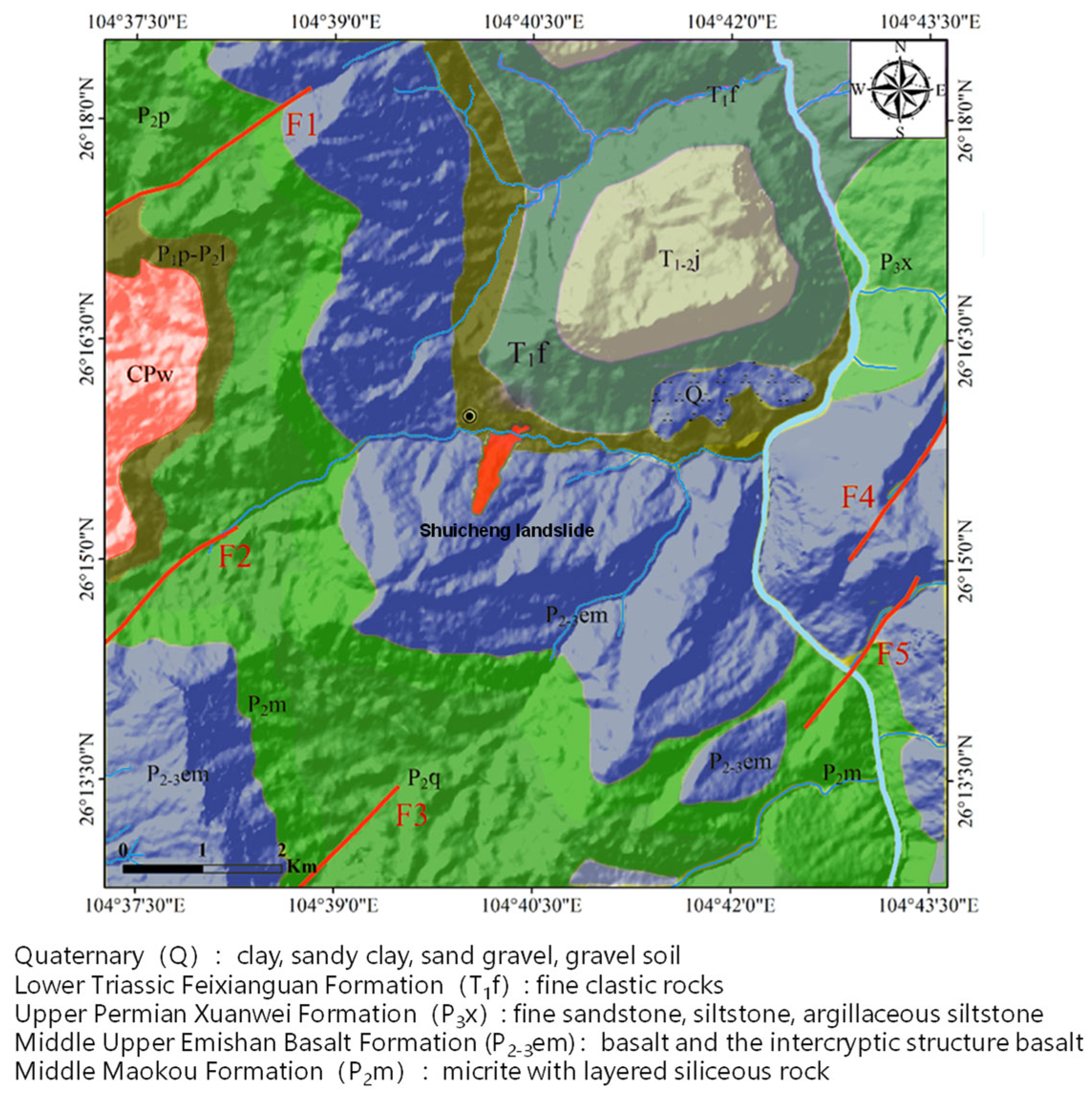
2.2. Geological and Topographical Conditions

The rockslide is in the Yangtze paraplatform. The Yangtze Platform is a platform formed by the Yangtze Cycle at the end of Late Proterozoic. The terrain of the Yangtze platform is high in the west and low in the east. Active tectonic movements make the geological condition complex with many faults. Therefore, the geological structure is controlled by faults and discontinuous planes, which further control the scale of landslides or debris flows. The lithology composition of the study area is mainly quaternary deposits, chaolite, basalt, and sandstone (Figure 2). After suffering from long-term tectonic movements, weathering, and seepage, the strength of the surface geological materials has become low, with many fractures in them. This is also one of the important reasons that geological disasters frequently occur in the study area.

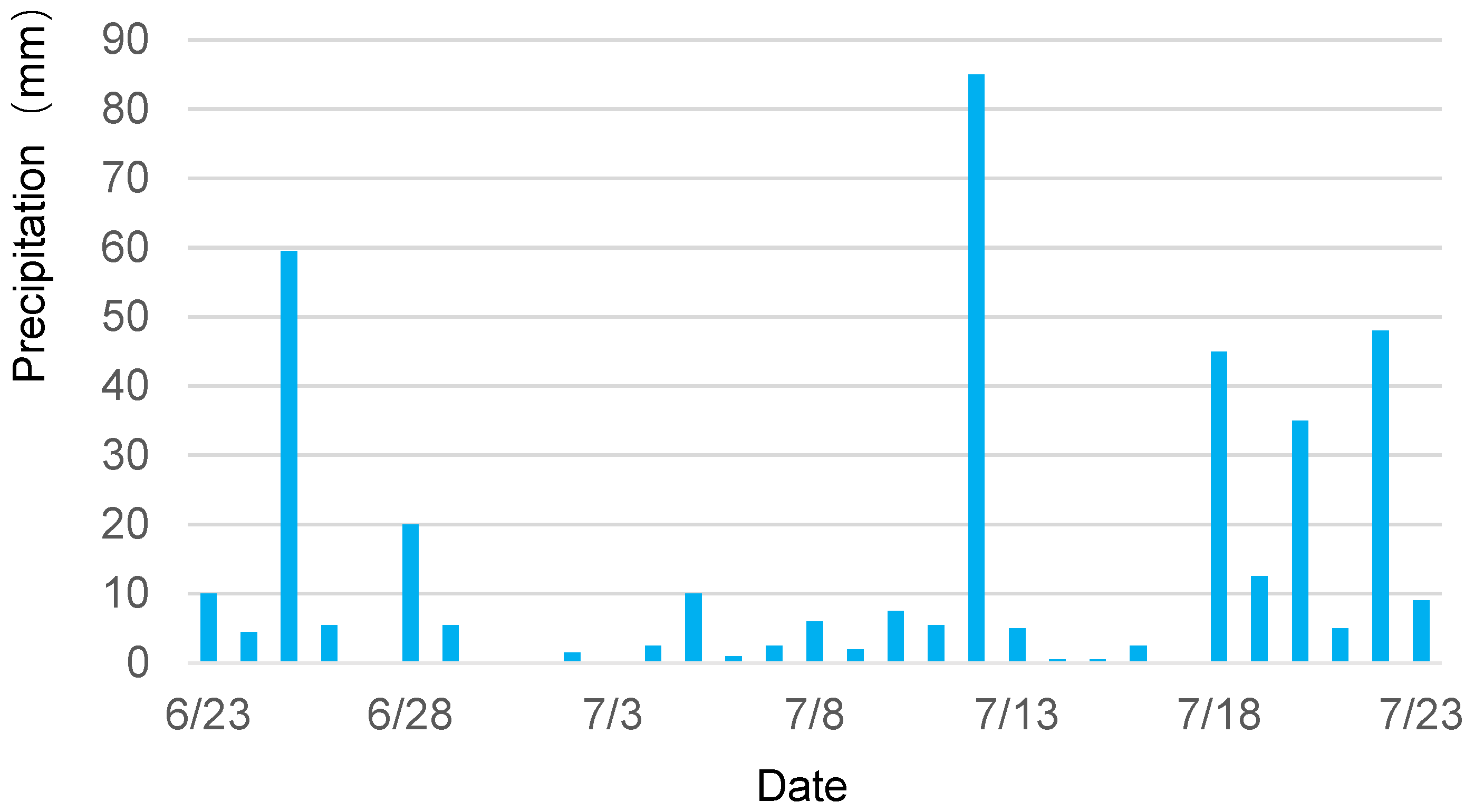
2.3. Rainfall Condition

The study area is the highland monsoon climate, with an average annual rainfall from 900 to 1500 mm, whose wet season is from June to August. Because rainfall is concentrated, landslides are usually triggered easily. One week before the landslide occurred, heavy rains occurred, with a precipitation of 287 mm in Jichang town (Figure 3). The heavy rainfall exacerbated the ground surface runoff. It not only reduced the strength of rocks and soils but also increased their density and finally made the landslide occur.

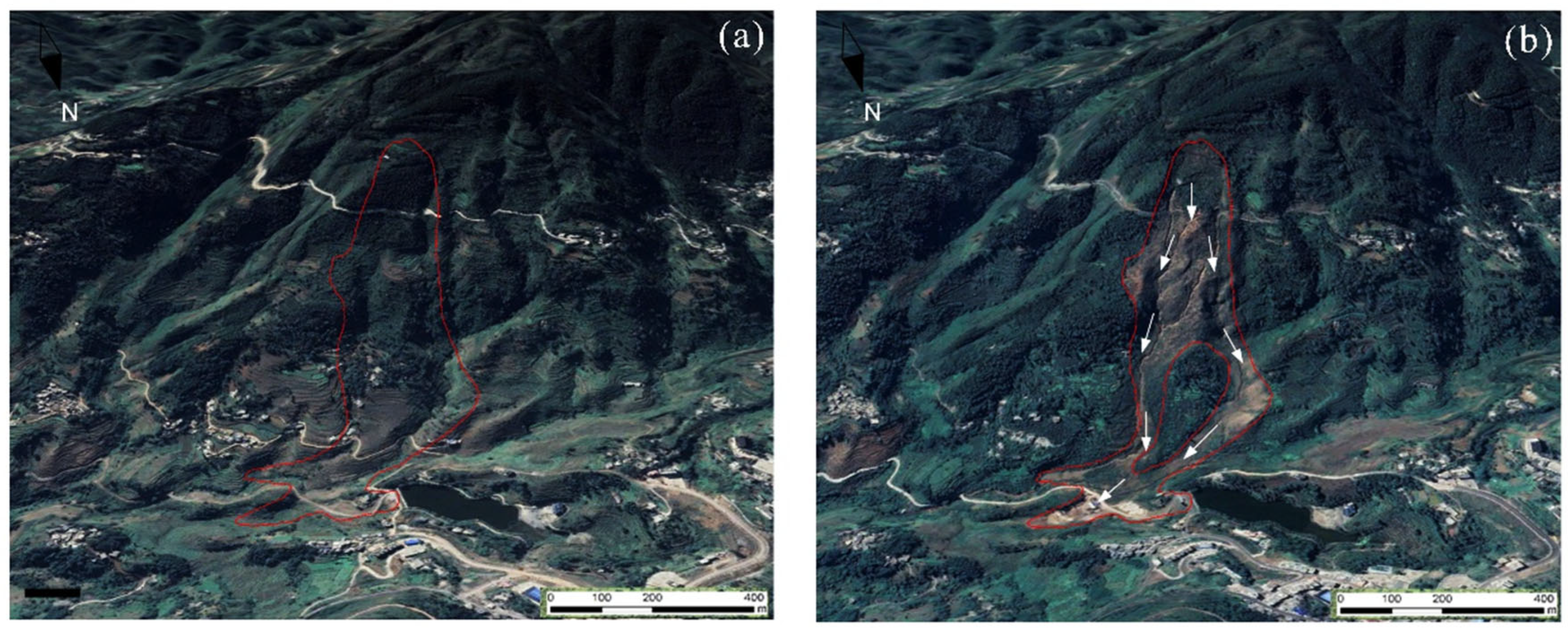
2.4. Jichang Rockslide

The Jichang rockslide occurred in a steep slope before the slope failure. The composition of the slope was block-layered basalt with a thickness of 2 m of quaternary deposits on it. The source area was located at a high part of the slope, whose elevation is from 1520 to 1665 m with an inclined angle of 50° (Figure 4). After the rockslide occurred, the rock materials moved out of the source area and formed a rockslide. The rockslide moved rapidly. When the rockslide reached an elevation of 1450 m, the sliding mass encountered a swelling terrain and was shunted into two different gullies. After passing the swelling terrain, the slides in the gullies converged together again, decelerating and being stopped in the wide gully terrain due to friction and collision. The final rockslide deposit, which had an average depth of 5 m and width of 350 m, had a run-out distance of 1350 m with an H/L ratio of 0.32.

Although the deposit area of the rockslide was clearly shown via field investigation and remote sensing images, its dynamic process has not been observed directly. The previous literature studied its run-out behavior by numerical simulations, using continuum methods such as the DISWM [29,30] and SPH [28]. However, these models cannot reflect the transition from a solid source to fluid slides clearly. In addition, dynamic fragmentation, the most important process in a rockslide, as well as corresponding quantitative parameters were not clearly reflected in previous numerical models. The FDEM has the potential to overcome the above shortcomings. Using it to investigate the dynamic process of the Jichang rockslide is novel and meaningful.

3. Methodology

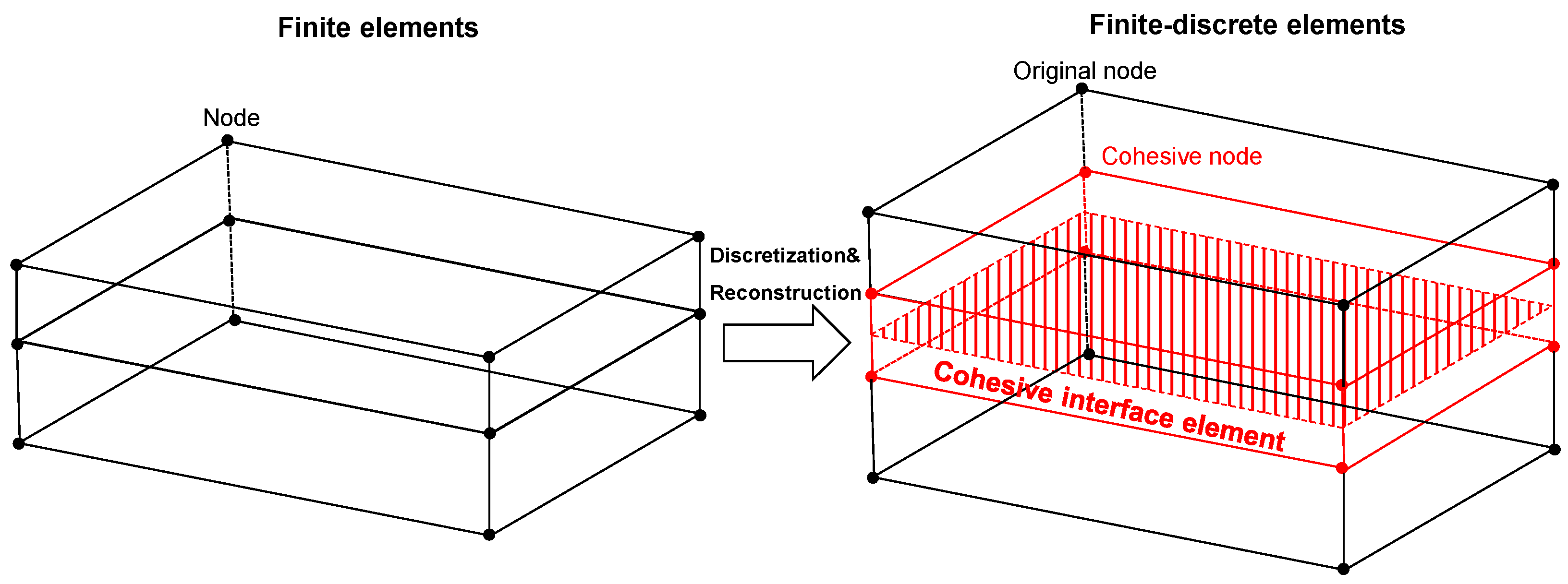
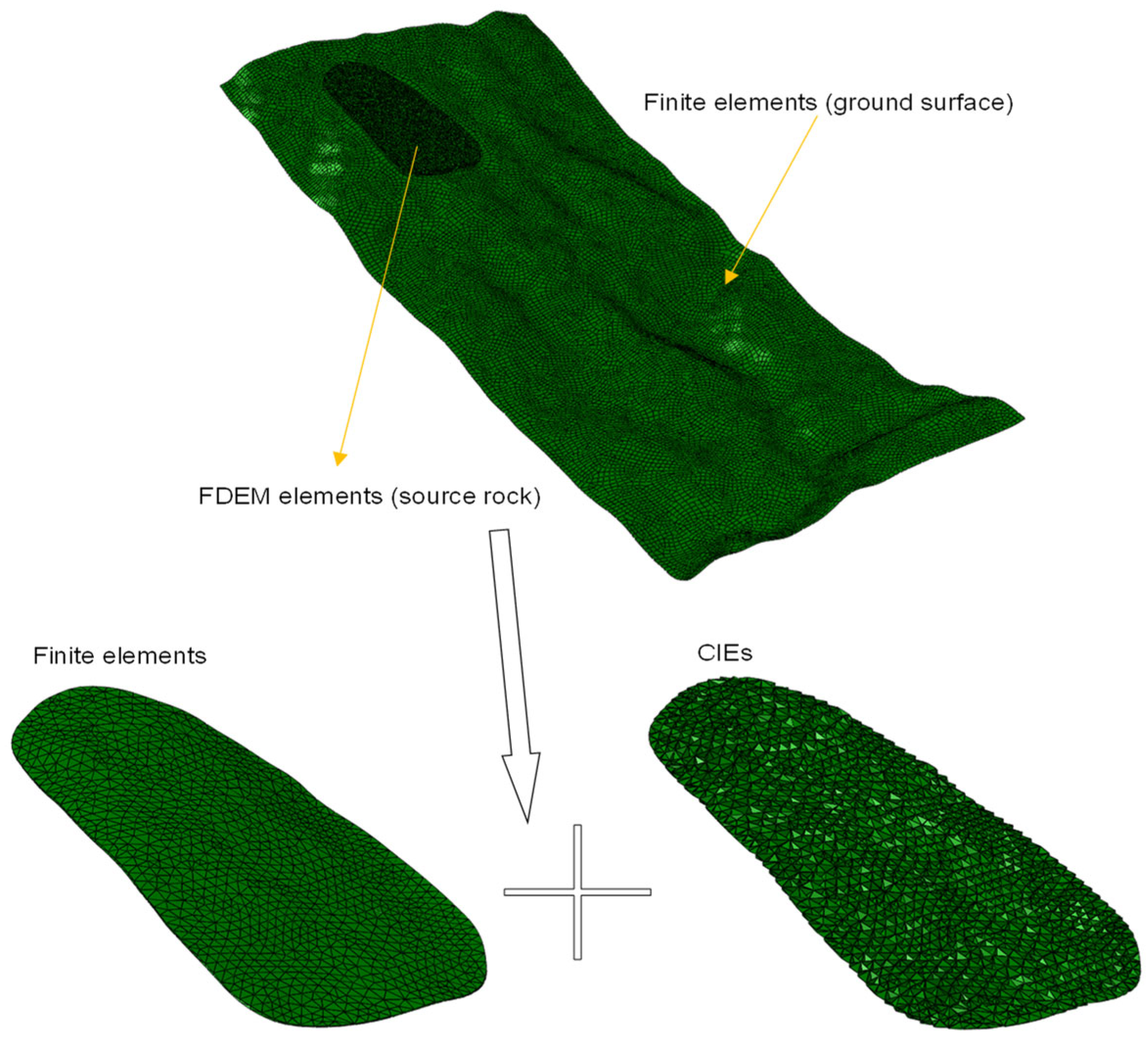
3.1. Finite-Discrete Element Method

The FDEM was first proposed by Munjiza et al. (1995) [27] for the fracturing behavior of solids such as rock. In this method, the solid was composed of two kinds of basic elements, i.e., finite elements and cohesive interface elements (CIEs). CIEs were inserted into the boundary of the finite elements and share nodes with surrounding finite elements (Figure 5). The finite elements in the FDEM focused on the deformation behavior, while the CIEs mainly described the damage and fracturing behaviors of the solid.

The constitutive equations of CIEs include a deformation period and a damage period when used to simulate rock. The deformation and damage behaviors are frequently described by a traction-separation constitutive response in a stress-displacement form [31,32]. A common form of a bilinearity traction-separation constitutive response is expressed as follows:

$$\left\{\begin{array}{c}t=k\delta \delta <{\delta }^0\\ t=\left(1-D\right)k\delta \delta \ge {\delta }^0\end{array}\right.$$

(1)

where $\mathit{t}$ is the traction stress, $k$ is the contact stiffness coefficient, $\mathit{\delta }$ is the traction displacement, ${\delta }^0$ is the displacement corresponding to the peak stress value, and D is the damage variable.

According to Equation (1), the CIE will deform as the conventional elastic finite elements before reaching a peak strength. After reaching the peak strength $k{\delta }^0$, the CIE will enter into a damage period and fracture energy, which is defined as the consumed energy for crack propagation per unit area, will be an important parameter. The CIE will be completely damaged when its consumed fracture energy reaches the maximum value $G^c$ and a crack will form. The damage variable of a CIE is defined as [33]:

$$D=\frac{\frac{2G^c}{T_{eff}^o}({\delta }_{max}-{\delta }^0)}{{\delta }_{max}(\frac{2G^c}{T_{eff}^o}-{\delta }^0)}$$

(2)

where $D$ is the damage variable, ${\delta }_{max}$ is the maximum displacement in the whole process, $G^c$ is the fracture energy, and $T_{eff}^o$ is the effective traction stress when damage is initialized.

A CIE can be damaged in the pure normal direction or tangential direction, representing tension fracture (mode I fracture) and in-plane shear fracture (mode II fracture), respectively. It can also be damaged in both the normal and tangential directions, representing a mixed-mode fracture. Once a CIE is damaged in both the normal and tangential directions, the quads damage failure criterion is used to determine the initial damage of the CIEs [31] (Equation (3)) and the quadratic power law is used to determine the complete damage of the CIEs (Equation (4)), which can be expressed as follows:

$${\left\{\frac{<{\mathit{t}}_{\mathit{n}}>}{t_n^o}\right\}}^2+{\left\{\frac{{\mathit{t}}_{\mathit{s}}}{t_s^o}\right\}}^2+{\left\{\frac{{\mathit{t}}_{\mathit{t}}}{t_t^o}\right\}}^2=1$$

(3)

$${\left\{\frac{G_n}{G_n^C}\right\}}^2+{\left\{\frac{G_s}{G_s^C}\right\}}^2+{\left\{\frac{G_t}{G_t^C}\right\}}^2=1$$

(4)

where $<{\mathrm{t}}_{\mathrm{n}}>$, ${\mathrm{t}}_{\mathrm{s}}$, and ${\mathrm{t}}_{\mathrm{t}}$ denote the normal compressive stress and two tangential traction stresses, respectively; ${\mathrm{t}}_{\mathrm{n}}^{\mathrm{o}}$, ${\mathrm{t}}_{\mathrm{s}}^{\mathrm{o}}$, and ${\mathrm{t}}_{\mathrm{t}}^{\mathrm{o}}$ denote the maximum normal and tangential traction stresses; ${\mathrm{G}}_{\mathrm{n}}^{\mathrm{C}},$ ${\mathrm{G}}_{\mathrm{s}}^{\mathrm{C}},$ and ${\mathrm{G}}_{\mathrm{t}}^{\mathrm{C}}$ denote the complete fracture energy in the normal and two tangential directions, respectively; and ${\mathrm{G}}_{\mathrm{n},}$ ${\mathrm{G}}_{\mathrm{s}},$ and ${\mathrm{G}}_{\mathrm{t}}$ are the real fracture energy in the normal and two tangential directions, respectively.

Once the CIE between two finite elements is damaged completely, the connected finite elements will be apart from each other, with a potential contact. Whether two separate finite elements make contact with each other depends on their node positions. If a node of one element penetrates the surface of the other element, a contact force will form. The magnitude of the normal contact force is determined by the node penetration distance to the surface. If relative tangential movement occurs, a tangential contact force will form and its magnitude is the product of the friction coefficient and normal contact force [6]. Displacement and velocity of the finite elements are updated according to Newton’s second law of movement based on an explicit central-difference integration rule. Detailed methods of the FDEM used in this paper were introduced in the authors’ previous literature [6].

3.2. Numerical Model Construction and Setting

The construction of the three-dimensional rockslide model relied on the digital terrain model (DTM) data before and after slope failure. The resolution of the DTM data was 5 m, which made the constructed three-dimensional model have an accurate terrain surface. The scale of the source material was determined by the pre-failure and post-failure terrain difference in the source area, while the slide and deposit area were determined by the pre-failure terrain data. The slide and deposit surface were set as the finite elements, while the source rock was set as the FDEM elements. The shape of the finite elements in the FDEM source rock was tetrahedron and its number was 15,765, with an average length of 5 m. The number of CIEs between finite elements was 29,105 (Figure 6). These CIEs represented the potential fracturing path of the material. The compositions of the finite elements of the source rock and ground surface were set as rock material. A group of empirical parameters, with a rock density of 2000 kg/m³, Young’s modulus of 38.7 GPa, and Poisson’s ratio of 0.25, was adopted for the simulation. The parameters of Young’s modulus and Poisson’s ratio did not affect the rockslide simulation at all because rock fragmentation and movement were the most significant movement behaviors while rock deformation could be ignored. The CIE parameters were obtained by referring to the other literature. According to the previous literature [11,31,32], the tension strength and shear strength of intact rock samples are frequently considered the same and their empirical values are from 8 MPa to 31.5 MPa. The fracture energy of mode II is frequently considered 5 times that of mode I, and their empirical values were from 100 N/m to 1000 N/m. Considering the rock mass of the Jichang landslide had relatively high weathering and had numerous discontinuities, its strength was much lower than that of the intact rock samples. The group’s lower mechanical values of ${\mathrm{t}}_{\mathrm{n}}$ and ${\mathrm{t}}_{\mathrm{s}}$ were adopted as 1 MPa, and ${\mathrm{G}}_{\mathrm{I}}^{\mathrm{C}}$ and ${\mathrm{G}}_{\mathrm{I}\mathrm{I}}^{\mathrm{C}}$ were adopted as 10 N/m and 50 N/m, respectively. Friction between rock materials was adopted as a value of 0.33, which was calibrated by back-analysis [28] and a laboratory test [29]. These parameters were calibrated by comparing the rockslide deposit area in the field investigation; this kind of back-analysis is considered as the most important calibrated way to prove the credibility of the parameters [4,34]. The simulation time of the rockslide run-out process was 75 s.

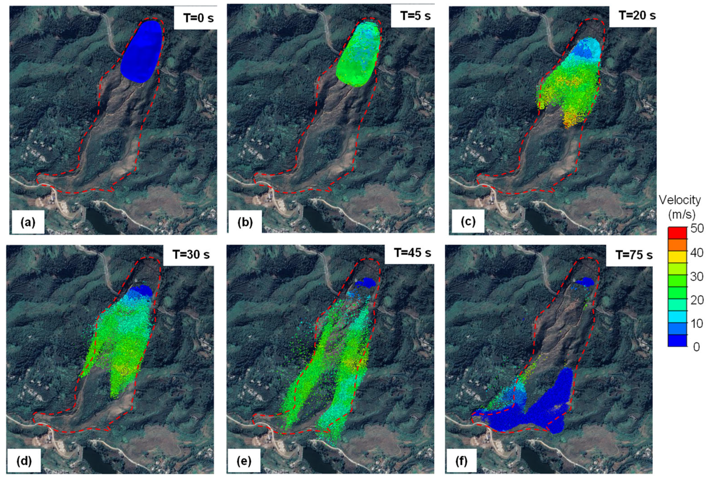
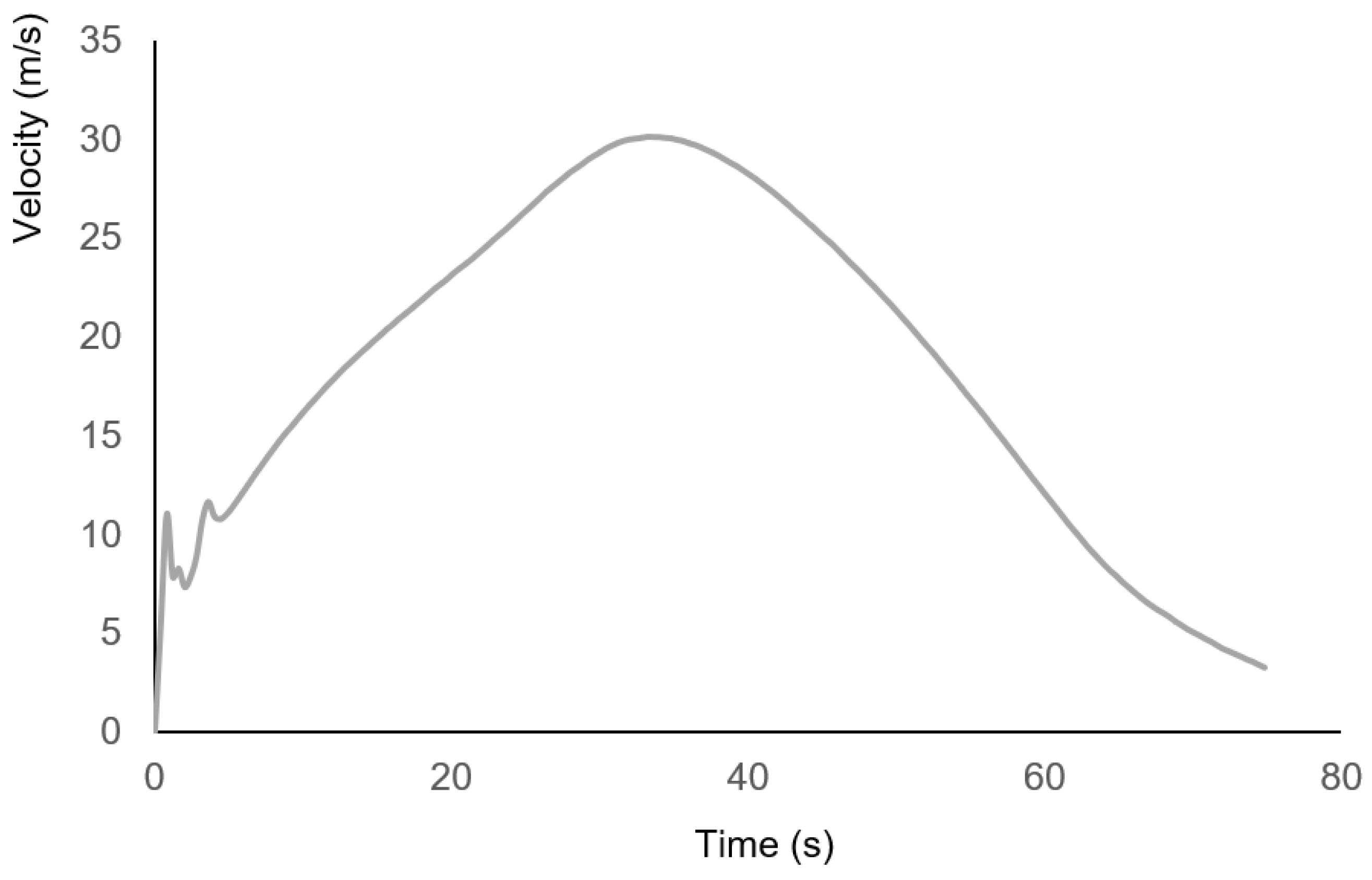
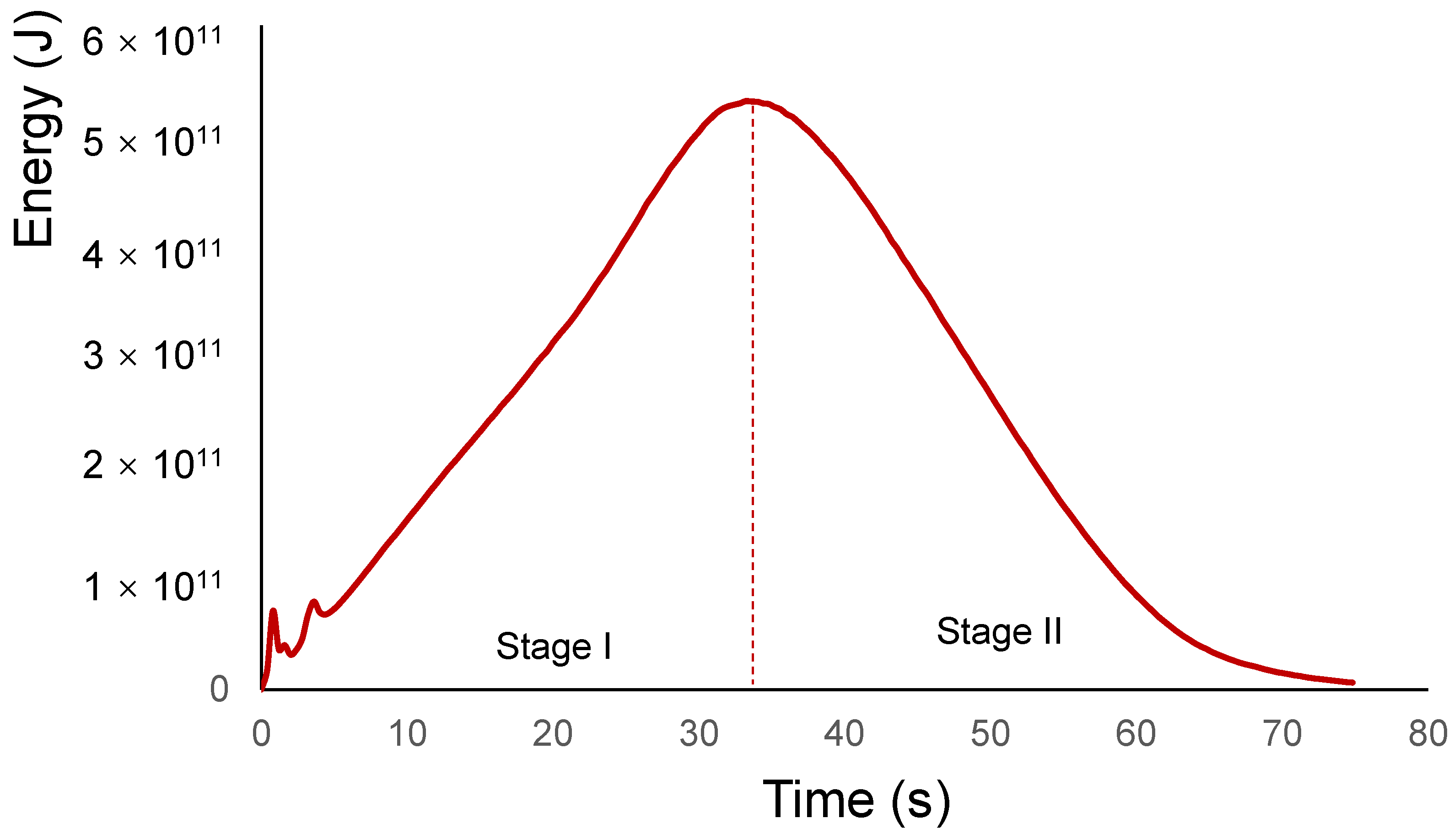
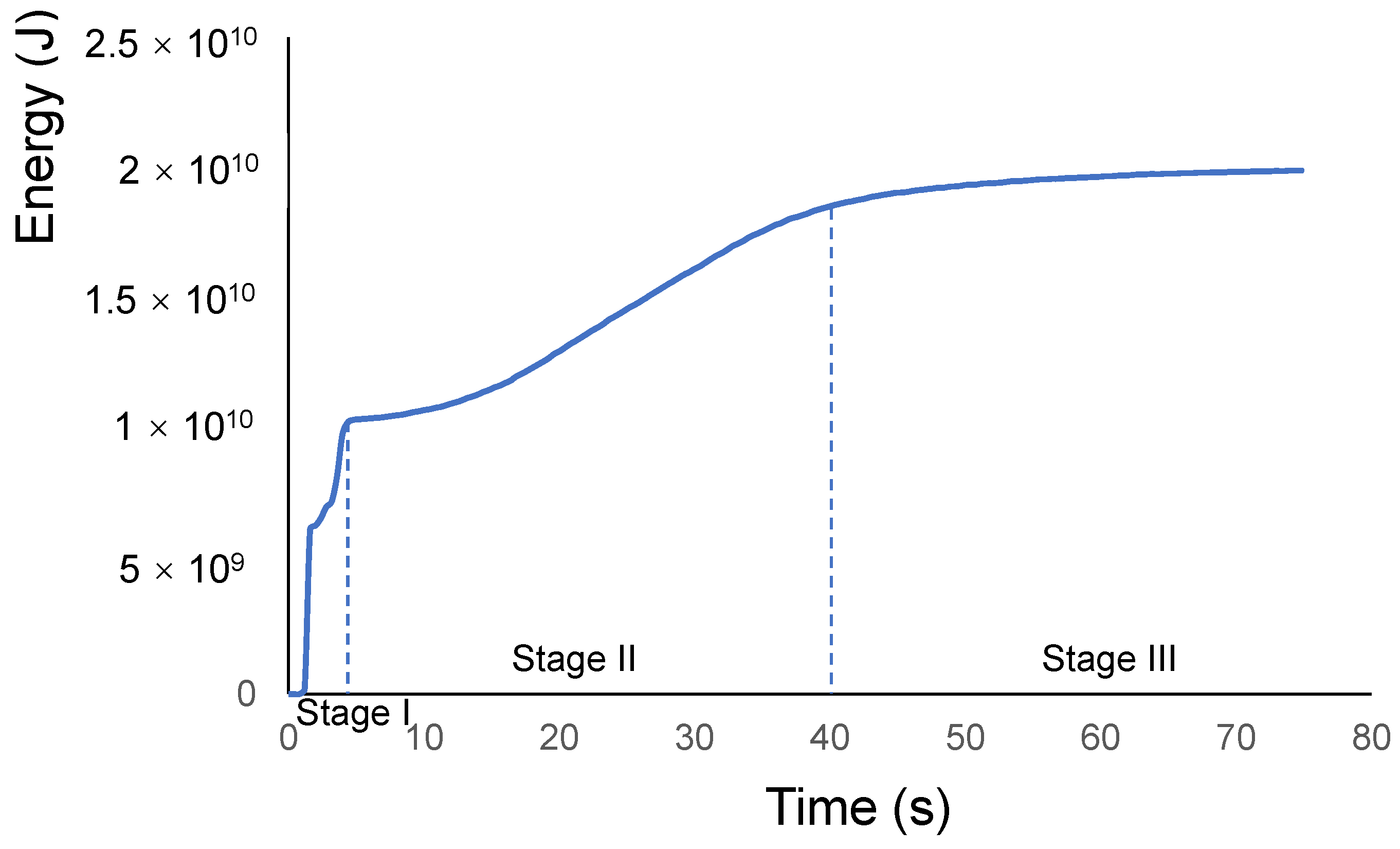
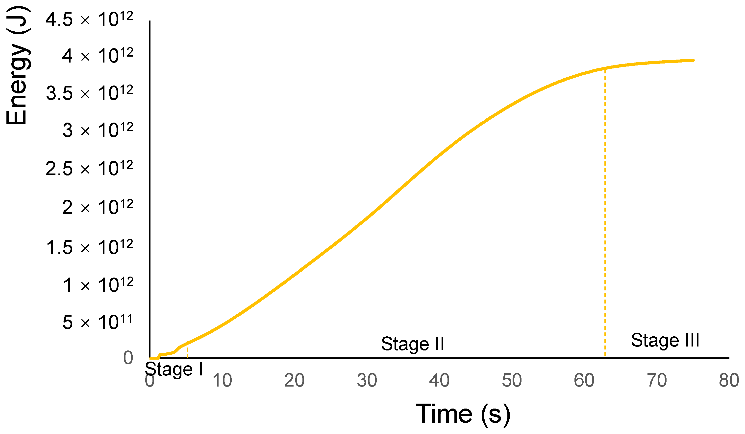
4. Numerical Simulation Results and Discussion

The typical run-out process of the Jichang rockslide is shown in Figure 7 and the initial state of the simulation is shown in Figure 7a. In addition, the average movement velocity of the rockslide is shown in Figure 8. After the simulation started, many cracks started forming in the source rock because of strong local compressive stress generated from a collision with irregular terrain, and it agreed with the real landslide situation (Figure 7b). At the time of 20 s, the source rock ran out of the source area. The source rock became very fragmental, and the front part of the sliding mass had obviously disintegrated to flow with a movement speed reaching 30 m/s. Because of the partial terrain bugle, the front part of the sliding mass had a trend to separate (Figure 7c). At 30 s, the sliding mass encountered a higher terrain bugle and, therefore, the sliding mass was completely separated by the terrain and ran into two gullies. At the same time, the sliding mass reached a peak speed at 30 s with a speed of 30 m/s (Figure 8). The rockslide moved along two different gullies, respectively (Figure 7d). The maximum speed of the partial slides reached 45 m/s. When they reached the wide gully at the bottom of the slope, the rockslides in the two gullies met and merged again. Due to the slower slope of the terrain, the front part of the sliding mass decelerated due to friction and collision with the topography (Figure 7e). After the front part of the sliding mass stopped moving, the movement of the subsequent sliding mass was gradually stopped by the front sliding mass. At 75 s, the rockslide was almost completely deposited (Figure 7f). In general, the simulated rock deposit area corresponded well with the landslide deposit area in the field investigation, indicating the simulation result is reasonable.

The physical variables of mass movement including kinetic energy (E_k), accumulated fracture energy generated by dynamic fragmentation (E_G), and accumulated friction energy (E_f) can be acquired from the FDEM simulation, and these variables can further reflect a rockslide dynamic process. Among them, E_k and E_f can be acquired from the conventional DEM method, but E_G is rarely shown. E_G is an important variable in rockslide simulations because dynamic fragmentation is considered as a most important process affecting a rockslide simulation. Dynamic fragmentation not only affects the transition from solid source to fluid slides but is also considered as a key factor making a rockslide have a high speed and long run-out distance [35,36,37,38]. Conventional DEM with the bonded particle model (BPM) [39] only considers fracture strength but does not consider fracture energy, making rockslide simulations based on this method not show the variation in fracture energy [40,41]. The variations in E_G, E_k, and E_f from the FDEM simulation are shown in Figure 9, Figure 10 and Figure 11, respectively.

According to the variation in E_k, the process of the Jichang rockslide can be considered as having two movement processes in general: the acceleration process and the deceleration process (Figure 9). The acceleration process lasted from 0 s to 33 s. It showed the process after the slope failure to the sliding mass encountering the terrain bugle and separating into two gullies. After the sliding mass separated into two gullies, several factors made the sliding mass start to decelerate. The first factor was that the front sliding mass constantly collided with the terrain bugle, reducing its ${\mathrm{E}}_{\mathrm{k}}$. The second factor was that the lower slope was gentler than the upper slope, making the kinetic energy consumption obviously increase on the lower slope path. The third reason was that lateral friction obviously increased between the sliding mass and the gully after the sliding mass ran into the gullies. Therefore, the sliding mass started to decelerate after 33 s and constantly decelerated until completely depositing.

As for E_G, it generally increased throughout the whole sliding process, and its variation can be divided into three stages from the aspect of the growth rate (Figure 10). In the initial 5 s, the increase in E_G was very rapid, with a growth rate of 2.17 × 10⁹ J/s, which is obviously greater than other stages. In this period, 54% of the total fracture energy was released, which indicated the fracturing process was very intense and the source material disintegration degree was very significant at 5 s. At the time of 5 s to 40 s, E_G still constantly increased at a relatively great rate of 2.26 × 10⁸ J/s, and 39% of the total fracture energy was released in this period. This period generally belonged to the acceleration period of the sliding mass. Therefore, under the movement conditions of high speed and long run-out distance, the fracturing process was still very intense. However, because of the size effect, a relatively complete and large source rock can generate fracture and break more easily, with more fracture energy being consumed. The source material fractured into many small fragments after 5 s; therefore, the growth rate of E_G from 5 to 40 s was obviously smaller than it was in the initial 5 s. After 40 s, the increase in E_G was very slow, with a growth rate of 3.11 × 10⁷ J/s, and 7% of the total fracture energy was released in this period. The reason the growth rate was very slow in this period was that the sliding mass entered the deceleration period, making E_G grow more slowly. The FDEM still provides an approach to calculate E_G in a rockslide, and its variation in the simulation is important to further realize the dynamic fragmentation mechanism and process.

As for E_f, it increased throughout the whole run-out process and can be divided into three stages from the aspect of the growth rate (Figure 11). The first stage was from 0 to 5 s with an E_f growth rate of 3.73 × 10¹⁰ J/s; the second stage was from 5 to 63 s with an E_f growth rate of 8.01 × 10¹⁰ J/s while the third stage was from 63 to 75 s with an E_f growth rate of 1 × 10¹⁰ J/s. The growth rate of E_f is related to the sliding mass movement speed and the fracturing degree of the source rock in general. After the rockslide initialized, the source rock started to move and the movement speed was small before 5 s. In this period, the fracturing rate of the source rock increased rapidly but relative movement between fragments was generally low; therefore, the growth rate of E_f was low. At 5 s, the source rock started to become very fragmental because a large amount of fracture energy had been generated. The intense dynamic fragmentation process made the contact surface area of relative movement increase sharply; therefore, E_f started to increase rapidly. From 5 to 60 s, the growth rate of E_f increased rapidly and reached the maximum value of 7.92 × 10¹⁰ J/s at 33 s. At this time, the sliding mass also reached its maximum kinetic energy, indicating that it reached its maximum movement speed. In addition, 89% of the total fracture energy was released at this time, indicating the source rock had almost completely disintegrated to form many new contact areas for relative movement. Under these conditions, relative movement displacements between fragmental blocks reached a maximum value, making the growth rate of E_f reach its maximum value. From 33 to 40 s, the movement speed of the sliding mass decreased while the fragmentation degree of the source rock increased, making the growth rate of E_f almost remain the same. After 40 s, the fragmentation degree of the source rock almost did not increase and the growth rate of E_f decreased with the mass movement speed. After 63 s, the rockslide almost stopped moving, making the relative movement distance between fragmental blocks become smaller, generating a much lower growth rate of E_f. It was found from the curves that E_f was much larger than E_G and E_k, indicating the high-position gravitational potential energy of the source rock was mainly dissipated in the form of friction energy. The friction energy was transformed into heat energy, making the temperature on the main slip surface rise sharply. The high temperature might make the slip surface generate thermal pressurization or steam lubrication [42], which further weakens friction between a sliding mass and slip surface, resulting in an excessive run-out speed and movement distance.

In the authors’ previous literature [28], an SPH simulation was conducted for the Jichang rockslide. SPH is a continuum method and rockslide simulation based on it frequently considering the sliding mass as the flow, using macroscopic governing equations such as the modified Navier–Stokes equations to describe mass movement behavior. The SPH simulation can be used as a case to represent the continuum models including DISWM to be compared with the FDEM simulation. In the SPH simulation, the sliding mass was treated as the Bingham fluid, a type of non-Newtonian fluid that begins to flow when the yield stress of the material is greater than a certain value. After starting to flow, the Bingham fluid has a linear fluidity variation, and it has been widely applied to landslide or rockslide simulations. Detailed settings of rockslide simulations based on the SPH approach have been clearly described in the previous literature [28].

Figure 12 shows the rockslide run-out scenarios in the FDEM simulation and SPH simulation at different times. It can be found that both of the simulations have similar run-out processes when the final simulated rock deposit area is calibrated by the real landslide deposit area. However, there are still some differences between these two models. From the scenarios at 20 s and 30 s, it was found that the rheology of the sliding mass in the SPH model was obviously higher than the sliding mass in the FDEM model at the initial run-out stage, indicated in the phenomenon that the rockslide sliding area in the SPH model was greater than that in the FDEM model. In addition, the maximum movement speed of the partial sliding mass reached 35 m/s in the SPH model from 20 to 30 s, greater than the value of 30 m/s in the FDEM model. When the run-out process proceeded, the sliding mass in the FDEM model presented a stronger dispersion due to the characteristics of the method. Many small blocks are scattered around the main sliding mass due to collision. As for the sliding mass in the SPH model, the sliding mass appeared more integrated because the method was the continuum method.

Although the run-out speeds were similar in both models, the manifestations of the two models were quite different. In the SPH model, the sliding mass moved like the fluid, but the sliding mass still existed as a solid motion in the FDEM model initially (Figure 12). The fragmentation and disintegration processes of the sliding mass could be clearly observed from the FDEM model. In addition, the fragmentation variables including the fracturing energy and damage degree as well damage mode, which were quantitatively acquired from the FDEM model, were not reflected by the SPH model and other continuum models. This means using the FDEM model to simulate rockslides or rock avalanches has the potential to study more complex movement mechanisms at the expense of many computational sources [43].

5. Conclusions

In this paper, the Jichang rockslide is simulated by a novel numerical approach for landslide simulation: the FDEM. The simulated rock deposit area is generally consistent with it in the field investigation based on back-analysis, indicating the FDEM can well solve a rockslide simulation. The results show the whole process of the rockslide is 75 s. The maximum movement speed of the sliding mass can reach 35 m/s, while partial slides can reach 45 m/s. Except for the movement speed information, the variation in the kinetic energy and fracture energy as well as accumulated friction energy can be acquired from the FDEM simulation. The sliding mass has two movement processes including the acceleration process and the deceleration process from the variation in the kinetic energy. The acceleration process lasts from 0 to 33 s, while the deceleration process lasts from 33 to 75 s. The dynamic fragmentation degree was high before 40 s. Of the total fracture energy, 54% is released in the first 5 s while 39% of the total fracture energy is released from 5 to 40 s. The accumulated friction energy of the sliding mass constantly increased in the run-out process, and it was greater than the kinetic energy and fracture energy in general. The phenomenon proves that the high-position gravitational potential energy of the sliding mass mainly converts into friction energy (heat energy).

References

1. Plafker, G.; Ericksen, G.E. Nevados Huascaran avalanches, Peru. In Rockslides and Avalanche; Voight, B., Ed.; Elsevier: Amsterdam, The Nertherland, 1987; pp. 277–314. [Google Scholar]
2. McDougall, S.; Hungr, O. Dynamic modelling of entrainment in rapid landslides. Can. Geotech. J. 2005, 42, 1437–1448. [Google Scholar] [CrossRef]
3. Ibañez, J.P.; Hatzor, Y.H. Rapid sliding and friction degradation: Lessons from the catastrophic Vajont landslide. Eng. Geol. 2018, 244, 96–106. [Google Scholar] [CrossRef]
4. Aaron, J.; McDougall, S. Rock avalanche mobility: The role of path material. Eng. Geol. 2019, 257, 105126. [Google Scholar] [CrossRef]
5. Shi, A.-W.; Wang, Y.-F.; Cheng, Q.-G.; Lin, Q.-W.; Li, T.-H.; Wünnemann, B. The largest rock avalanche in China at Iymek, Eastern Pamir, and its spectacular emplacement landscape. Geomorphology 2023, 421, 108521. [Google Scholar] [CrossRef]
6. Bao, Y.; Chen, J.; Su, L.; Zhang, W.; Zhan, J. A novel numerical approach for rockslide blocking river based on the CEFDEM model: A case study from the Samaoding paleolandslide blocking river event. Eng. Geol. 2023, 312, 106949. [Google Scholar] [CrossRef]
7. Bao, Y.; Su, L.; Chen, J.; Ouyang, C.; Yang, T.; Lei, Z.; Li, Z. Dynamic process of a high-level landslide blocking river event in a deep valley area based on FDEM-SPH coupling approach. Eng. Geol. 2023, 319, 107108. [Google Scholar] [CrossRef]
8. Fang, K.; Zhang, J.; Tang, H.; Hu, X.; Yuan, H.; Wang, X.; An, P.; Ding, B. A quick and low-cost smartphone photogrammetry method for obtaining 3D particle size and shape. Eng. Geol. 2023, 322, 107170. [Google Scholar] [CrossRef]
9. Wang, C.; Wang, H.; Qin, W.; Wei, S.; Tian, H.; Fang, K. Behaviour of pile-anchor reinforced landslides under varying water level, rainfall, and thrust load: Insight from physical modelling. Eng. Geol. 2023, 325, 107293. [Google Scholar] [CrossRef]
10. Wang, Y.; Lin, Q.; Li, K.; Shi, A.; Li, T.; Cheng, Q. Review on Rock Avalanche Dynamics. J. Earth Sci. Environ. 2021, 43, 164–181. (In Chinese) [Google Scholar]
11. Wu, Z.; Ma, L.; Fan, L. Investigation of the characteristics of rock fracture process zone using coupled FEM/DEM method. Eng. Fract. Mech. 2018, 200, 355–374. [Google Scholar] [CrossRef]
12. Wu, J.-H.; Hsieh, P.-H. Simulating the postfailure behavior of the seismically- triggered Chiu-fen-erh-shan landslide using 3DEC. Eng. Geol. 2021, 287, 106113. [Google Scholar] [CrossRef]
13. Fang, K.; Tang, H.; Li, C.; Su, X.; An, P.; Sun, S. Centrifuge modelling of landslides and landslide hazard mitigation: A review. Geosci. Front. 2023, 14, 101493. [Google Scholar] [CrossRef]
14. Do, T.N.; Wu, J.-H. Simulating a mining-triggered rock avalanche using DDA: A case study in Nattai North, Australia. Eng. Geol. 2019, 264, 105386. [Google Scholar] [CrossRef]
15. Peng, X.; Liu, J.; Cheng, X.; Yu, P.; Zhang, Y.; Chen, G. Dynamic modelling of soil-rock-mixture slopes using the coupled DDA-SPH method. Eng. Geol. 2022, 307, 106772. [Google Scholar] [CrossRef]
16. Tang, C.-L.; Hu, J.-C.; Lin, M.-L.; Angelier, J.; Lu, C.-Y.; Chan, Y.-C.; Chu, H.-T. The Tsaoling landslide triggered by the Chi-Chi earthquake, Taiwan: Insights from a discrete element simulation. Eng. Geol. 2009, 106, 1–19. [Google Scholar] [CrossRef]
17. Han, X.; Chen, J.; Xu, P.; Zhan, J. A well-balanced numerical scheme for debris flow run-out prediction in Xiaojia Gully considering different hydrological designs. Landslides 2017, 14, 2105–2114. [Google Scholar] [CrossRef]
18. Ouyang, C.; An, H.; Zhou, S.; Wang, Z.; Su, P.; Wang, D.; Cheng, D.; She, J. Insights from the failure and dynamic characteristics of two sequential landslides at Baige village along the Jinsha River, China. Landslides 2019, 16, 1397–1414. [Google Scholar] [CrossRef]
19. Conte, E.; Pugliese, L.; Troncone, A. Post-failure stage simulation of a landslide using the material point method. Eng. Geol. 2019, 253, 149–159. [Google Scholar] [CrossRef]
20. Li, X.; Yan, Q.; Zhao, S.; Luo, Y.; Wu, Y.; Wang, D. Investigation of influence of baffles on landslide debris mobility by 3D material point method. Landslides 2020, 17, 1129–1143. [Google Scholar] [CrossRef]
21. Pastor, M.; Haddad, B.; Sorbino, G.; Cuomo, S.; Drempetic, V. A depth-integrated, coupled SPH model for flow-like landslides and related phenomena. Int. J. Numer. Anal. Methods Géoméch. 2009, 33, 143–172. [Google Scholar] [CrossRef]
22. Bao, Y.; Su, L.; Chen, J.; Zhang, C.; Zhao, B.; Zhang, W.; Zhang, J.; Hu, B.; Zhang, X. Numerical investigation of debris flow–structure interactions in the Yarlung Zangbo River valley, north Himalaya, with a novel integrated approach considering structural damage. Acta Geotech. 2023, 18, 5859–5881. [Google Scholar] [CrossRef]
23. Wang, Y.C.; Ju, N.P.; Zhao, J.J.; Xiang, X.Q. Formation mechanism of landslide above the mined out area in gentle inclined coal beds. J. Eng. Geol. 2013, 21, 61–68. [Google Scholar]
24. Zhao, J.J.; Ma, Y.T.; Lin, B.; Lan, Z.Y.; Shi, W.B. Geomechanical mode of mining landslides with gently counter-inclined bedding—A case study of Madaling landslide in Guizhou Province. Chin. J. Rock Mech. Eng. 2016, 35, 2217–2224. [Google Scholar]
25. Corominas, J.; Mavrouli, O.; Ruiz-Carulla, R. Magnitude and frequency relations: Are there geological constraints to the rockfall size? Landslides 2018, 15, 829–845. [Google Scholar] [CrossRef]
26. Gili, J.A.; Ruiz-Carulla, R.; Matas, G.; Moya, J.; Prades, A.; Corominas, J.; Lantada, N.; Núñez-Andrés, M.A.; Buill, F.; Puig, C.; et al. Rockfalls: Analysis of the block fragmentation through field experiments. Landslides 2022, 19, 1009–1029. [Google Scholar] [CrossRef]
27. Munjiza, A.; Owen, D.; Bicanic, N. A combined finite-discrete element method in transient dynamics of fracturing solids. Eng. Comput. 1995, 12, 145–174. [Google Scholar] [CrossRef]
28. Bao, Y.; Wang, H.; Su, L.; Geng, D.; Yang, L.; Shao, P.; Li, Y.; Du, N. Comprehensive analysis using multiple-integrated techniques on the failure mechanism and dynamic process of a long run-out landslide: Jichang landslide case. Nat. Hazards 2022, 112, 2197–2215. [Google Scholar] [CrossRef]
29. Gao, Y.; Li, B.; Gao, H.; Chen, L.; Wang, Y. Dynamic characteristics of high-elevation and long-runout landslides in the Emeishan basalt area: A case study of the Shuicheng “7.23” landslide in Guizhou China. Landslides 2020, 17, 1663–1677. [Google Scholar] [CrossRef]
30. Zhang, Y.; Xing, A.; Jin, K.; Zhuang, Y.; Bilal, M.; Xu, S.; Zhu, Y. Investigation and dynamic analyses of rockslide-induced debris avalanche in Shuicheng, Guizhou, China. Landslides 2020, 17, 2189–2203. [Google Scholar] [CrossRef]
31. Ma, G.; Zhou, W.; Ng, T.-T.; Cheng, Y.-G.; Chang, X.-L. Microscopic modeling of the creep behavior of rockfills with a delayed particle breakage model. Acta Geotech. 2015, 10, 481–496. [Google Scholar] [CrossRef]
32. Xi, X.; Yang, S.; Mcdermott, C.I.; Shipton, Z.K.; Fraser-Harris, A.; Edlmann, K. Modelling rock fracture induced by hydraulic pulses. Rock Mech. Rock Eng. 2021, 54, 3977–3994. [Google Scholar] [CrossRef]
33. Dassault Systèmes Inc. Abaqus 6.14 Online Documentation. Abaqus Analysis User’s Guide; Dassault Systèmes Inc.: Velizy-Villacoublay, France, 2014. [Google Scholar]
34. McDougall, S. 2014 Canadian Geotechnical Colloquium: Landslide runout analysis—Current practice and challenges. Can. Geotech. J. 2014, 54, 605–620. [Google Scholar] [CrossRef]
35. Davies, T.R.; McSaveney, M.J.; Hodgson, K.A. A fragmentation-spreading model for long-runout rock avalanches. Can. Geotech. J. 1999, 36, 1096–1110. [Google Scholar] [CrossRef]
36. Dufresne, A.; Davies, T. Longitudinal ridges in mass movement deposits. Geomorphology 2009, 105, 171–181. [Google Scholar] [CrossRef]
37. Dufresne, A.; Davies, T.R.H.; Mcsaveney, M.J. Influence of runout-path material on emplacement of the round top rock avalanche, New Zealand. Earth Surf. Process. Landf. 2010, 35, 190–201. [Google Scholar] [CrossRef]
38. Dufresne, A. Granular flow experiments on the interaction with stationary runout path materials and comparison to rock avalanche events. Earth Surf. Process. Landforms 2012, 37, 1527–1541. [Google Scholar] [CrossRef]
39. Potyondy, D.; Cundall, P. A bonded-particle model for rock. Int. J. Rock Mech. Min. Sci. 2004, 41, 1329–1364. [Google Scholar] [CrossRef]
40. Lu, C.Y.; Tang, C.L.; Chan, Y.C.; Hu, J.C.; Chi, C.C. Forecasting landslide hazard by the 3D discrete element method: A case study of the unstable slope in the Lushan hot spring district, Central Taiwan. Eng. Geol. 2014, 183, 14–30. [Google Scholar] [CrossRef]
41. Wei, J.; Zhao, Z.; Xu, C.; Wen, Q. Numerical investigation of landslide kinetics for the recent Mabian landslide (Sichuan, China). Landslides 2019, 16, 2287–2298. [Google Scholar] [CrossRef]
42. Hu, W.; Huang, R.; McSaveney, M.; Yao, L.; Xu, Q.; Feng, M.; Zhang, X. Superheated steam, hot CO2 and dynamic recrystallization from frictional heat jointly lubricated a giant landslide: Field and experimental evidence. Earth Planet. Sci. Lett. 2019, 510, 85–93. [Google Scholar] [CrossRef]
43. Hu, Y.-X.; Yu, Z.-Y.; Zhou, J.-W. Numerical simulation of landslide-generated waves during the 11 October 2018 Baige landslide at the Jinsha River. Landslides 2020, 17, 2317–2328. [Google Scholar] [CrossRef]
Figure 1. Jichang rockslide. The photos (a,b) represent the pre-failure and post-failure overviews, respectively (the pre-failure image was taken on 14 November 2018 and the post-failure image was taken on 11 October 2020). Red lines denote to landslide scale while white arrows denote to landslide movement direction.
Remotesensing 15 05708 g001
Figure 2. Geologic map of the study area (revised from Bao et al., 2022 [28]).
Remotesensing 15 05708 g002
Figure 3. Monthly rainfall data of the Jichang rockslide from 23 June to 23 July in 2019.
Remotesensing 15 05708 g003
Figure 4. Deposit characteristics of Jichang rockslide.
Remotesensing 15 05708 g004
Figure 5. Numerical sketch of the FDEM.
Remotesensing 15 05708 g005
Figure 6. Numerical model for the Jichang rockslide based on FDEM.
Remotesensing 15 05708 g006
Figure 7. Run-out scenarios of the Jichang rockslide based on the contour map of material and movement speed, respectively ((a) T = 0 s; (b) T = 5 s; (c) T = 20 s; (d) T = 30 s; (e) T = 45 s; (f) T = 75 s).
Remotesensing 15 05708 g007
Figure 8. Average movement velocity of the rockslide.
Remotesensing 15 05708 g008
Figure 9. Variation in the kinetic energy of the rockslide.
Remotesensing 15 05708 g009
Figure 10. Variation in the fracture energy of the rockslide.
Remotesensing 15 05708 g010
Figure 11. Variation in the friction energy of the rockslide.
Remotesensing 15 05708 g011
Figure 12. Comparison of FDEM and SPH simulation scenarios at different times.
Remotesensing 15 05708 g012
Disclaimer/Publisher’s Note: The statements, opinions and data contained in all publications are solely those of the individual author(s) and contributor(s) and not of MDPI and/or the editor(s). MDPI and/or the editor(s) disclaim responsibility for any injury to people or property resulting from any ideas, methods, instructions or products referred to in the content.