Article

Estimating the SPAD of Litchi in the Growth Period and Autumn Shoot Period Based on UAV Multi-Spectrum

1
College of Electronic Engineering (College of Artificial Intelligence), South China Agricultural University, Guangzhou 510642, China
2
Guangdong Laboratory for Lingnan Modern Agriculture, South China Agricultural University, Guangzhou 510642, China
3
Zhujiang College, South China Agricultural University, Guangzhou 510900, China
4
College of Horticulture, South China Agricultural University, Guangzhou 510642, China
5
College of Engineering, South China Agricultural University, Guangzhou 510642, China
*
Author to whom correspondence should be addressed.
Remote Sens. 2023, 15(24), 5767; https://doi.org/10.3390/rs15245767
Submission received: 4 September 2023 / Revised: 12 December 2023 / Accepted: 14 December 2023 / Published: 17 December 2023
(This article belongs to the Special Issue Advanced Sensing and Image Processing in Agricultural Applications)

Abstract

:
The relative content of chlorophyll, assessed through the soil and plant analyzer development (SPAD), serves as a reliable indicator reflecting crop photosynthesis and the nutritional status during crop growth and development. In this study, we employed machine learning methods utilizing unmanned aerial vehicle (UAV) multi-spectrum remote sensing to predict the SPAD value of litchi fruit. Input features consisted of various vegetation indices and texture features during distinct growth periods, and to streamline the feature set, the full subset regression algorithm was applied for dimensionality reduction. Our findings revealed the superiority of stacking models over individual models. During the litchi fruit development period, the stacking model, incorporating vegetation indices and texture features, demonstrated a validation set coefficient of determination (R2) of 0.94, a root mean square error (RMSE) of 2.4, and a relative percent deviation (RPD) of 3.0. Similarly, in the combined litchi growing period and autumn shoot period, the optimal model for estimating litchi SPAD was the stacking model based on vegetation indices and texture features, yielding a validation set R2, RMSE, and RPD of 0.84, 3.9, and 1.9, respectively. This study furnishes data support for the precise estimation of litchi SPAD across different periods through varied combinations of independent variables.

1. Introduction

Litchi, an economically significant crop with a rich historical legacy, boasts an average annual output exceeding 2 million tons in China. The country stands as the global leader in litchi production, contributing to over half of the world’s total output. Among the various litchi-producing regions in China, Guangdong Province takes the lead with the highest annual litchi production [1,2,3]. The cultivation of litchi necessitates sufficient water, with an optimal annual precipitation range falling between 1500 to 1800 mm. Litchi exhibits versatility in its soil preferences, showing adaptability to various soil types including mountain soil, red loam, yellow loam, flat sandy loam, and others [4,5]. Being a subtropical plant, litchi imposes stringent light requirements. Ideally, the cultivation area should receive an annual sunshine duration exceeding 1700 h, ensuring ample light throughout the growth and development phases of litchi fruit. Sunny weather during this critical period is essential, as abundant light significantly promotes photosynthesis, leading to the increased accumulation of photosynthetic substances in litchi fruit and thereby enhancing overall fruit quality [6,7].
During the growth of litchi, light stands out as the most pivotal factor. Investigating the vigor of litchi photosynthesis holds significant importance for the precise management of litchi quality. Chlorophyll, an indispensable pigment in crop photosynthesis, serves as a key determinant. The chlorophyll content aptly mirrors the extent of crop photosynthesis and the nutritional status during growth and development. The relative content of chlorophyll, as gauged by the soil and plant analyzer development (SPAD), is directly and intimately linked to chlorophyll content. Consequently, measuring litchi SPAD emerges as a nondestructive and reliable method, offering an indirect yet insightful means to assess chlorophyll content and, to a certain extent, reflect the degree of photosynthesis [8,9].
In recent years, an increasing number of scholars have employed machine learning methods to predict various crop phenotypic information. Hassanijalilian et al. [10] innovatively combined image processing with machine learning techniques to propose a streamlined and cost-effective method for calculating soybean chlorophyll levels in the field using a smartphone camera. They gathered a dataset comprising 720 soybean leaf images and corresponding SPAD readings. The results indicated that the support vector machine (SVM) model demonstrated the most robust validation performance (R2 = 0.89 and RMSE = 2.90 SPAD units). However, the process of capturing images in the field using smartphones was time-consuming, necessitating further in-depth experiments. While machine learning methods can achieve predictions of crop phenotypic information to a certain extent, it is worth noting that more advanced equipment is often required for large-scale prediction tasks [11].
With the rapid development of agricultural information technology, the establishment of a modern agricultural development system has emerged as a focal point in current Chinese agricultural research. Notably, low-altitude remote sensing technology is extensively utilized in the realm of intelligent agriculture through the use of unmanned aerial vehicles (UAVs) [12,13]. UAVs equipped with multi-spectral cameras capture remote sensing images, and the information extracted from these images is subsequently analyzed to enhance the guidance of field operations and overall management [14,15,16]. In the study from Jiang et al. [17], they employed four commonly used machine learning algorithms (RF, enet, ANN, PLSR) to predict phenotypic parameters such as PDM, PNA, and NNI. The results revealed that RF demonstrated the highest accuracy during the jointing and booting periods of wheat. However, it is noteworthy that the accuracy of the RF model was not entirely satisfactory, and no exploration of additional machine learning methods was conducted, leaving room for further research in this area. The aforementioned studies underscore the utility of integrating UAV remote sensing technology with diverse machine learning methods for predicting crop phenotypic information.
Leveraging UAV remote sensing technology in conjunction with machine learning methods for predicting crop SPAD values is a prominent research avenue, with many scholars having already undertaken relevant studies in this field. Huang et al. [18] introduced a method to estimate the chlorophyll content of Brassica napus using UAV RGB images. However, the study focused solely on the wintering period, prompting the need for subsequent investigations that encompass multi-period chlorophyll content measurements. Poudyal et al. [19] demonstrated that UAV hyperspectral imagery holds promise as a tool for predicting sugarcane morphophysiological traits. In comparison to other traits, this study highlighted that SPAD was predicted with the highest accuracy. Various algorithms, including ridge regression, linear regression, and support vector regression, were employed to predict sugarcane SPAD. Nevertheless, it is essential to note that the ridge regression algorithm has certain limitations. While it secures a more reliable regression coefficient, this comes at the cost of sacrificing some information and diminishing overall accuracy. In the study from Zhang Liyuan et al. [20], they conducted a more in-depth assessment of the sensitivity between maize chlorophyll and the structure of maize under water stress using UAV visualization technology. This study offers valuable research support for future predictions of maize SPAD. In the study from Shen Lanzhi et al. [21], they performed preprocessing on hyperspectral data using a combination of wavelet packet denoising, first-order derivative transformation, and principal component analysis. The results indicated that this preprocessing approach enhanced the accuracy and stability of the PLSR model. The aforementioned scholars contribute a solid research foundation and valuable experience in predicting crop SPAD values, providing a reference for the investigation into litchi SPAD prediction in this paper. This underscores that the amalgamation of UAV remote sensing and machine learning methods holds significant application value in predicting litchi SPAD.
However, currently, the primary focus of SPAD prediction research revolves around crops such as soybean, wheat, Brassica napus, sugarcane, and others. There is relatively limited research on employing ensemble learning methods to predict litchi SPAD values. Many scholars have tended to predict SPAD values using individual machine learning algorithms, which has the drawback of lower model accuracy. Therefore, there is a need for further enhancement in the accuracy of these models.
To enhance model accuracy, certain scholars have employed ensemble learning methods. Fei et al. [22] investigated the potential of merging hyperspectral reflectance with the EB-MA (energy-based model averaging) method for predicting wheat yield. Simultaneously, combining linear and nonlinear models exhibited superior performance compared to integrating a single type of machine learning model. In another study, a high-precision and highly reliable soybean meteorological yield prediction model framework was constructed using three effective machine learning algorithms (k-nearest neighbor algorithm, random forest algorithm, and support vector machine algorithm) as base models, employing stacking ensemble learning. This approach yielded commendable prediction results [23]. However, due to variations in test subjects and datasets, the determination coefficient R2 in the training outcomes of the ensemble learning model is not sufficiently high. Notably, there is a scarcity of research on predicting litchi SPAD values using the ensemble learning method at present.
In the context of litchi fruit growth and the autumn shoot period, this study acquired remote sensing images of the litchi canopy utilizing UAV multi-spectral technology. Subsequently, the obtained remote sensing images were processed with ENVI software, and spectral reflectance was extracted. Suitable vegetation indexes were identified through the full subset regression method. Simultaneously, considering the contemporaneously measured SPAD values of litchi canopy leaves on the ground, SPAD estimation models for litchi canopy leaves were primarily constructed using stacking and bagging algorithms. The accuracy levels of these models were then compared with traditional machine learning methods (SVR, RF, KNR, RR) to assess the advantages of the ensemble learning algorithm. This comprehensive approach aims to offer data support for litchi SPAD estimation.

2. Materials and Methods

2.1. Overview of the Study Area

The experimental area was situated at the Changgangshan Litchi Variety Garden, South China Agricultural University, Tianhe District, Guangzhou City, Guangdong Province (Figure 1). Geographically, it is positioned at 23°16′N, 113°34′E, experiencing an oceanic subtropical monsoon climate with an average annual temperature of 22 °C. The litchi trees in this area ranged from 10 to 15 years old, with an average tree height of 4 m. They consistently yielded well, and the soil type was identified as red soil. There were no specific requirements stipulated for irrigation amounts, fertilization types, fertilizer quantities, or other field management practices.

2.2. Measurement Method of the Litchi SPAD Value Based on the Integration of Space and Land

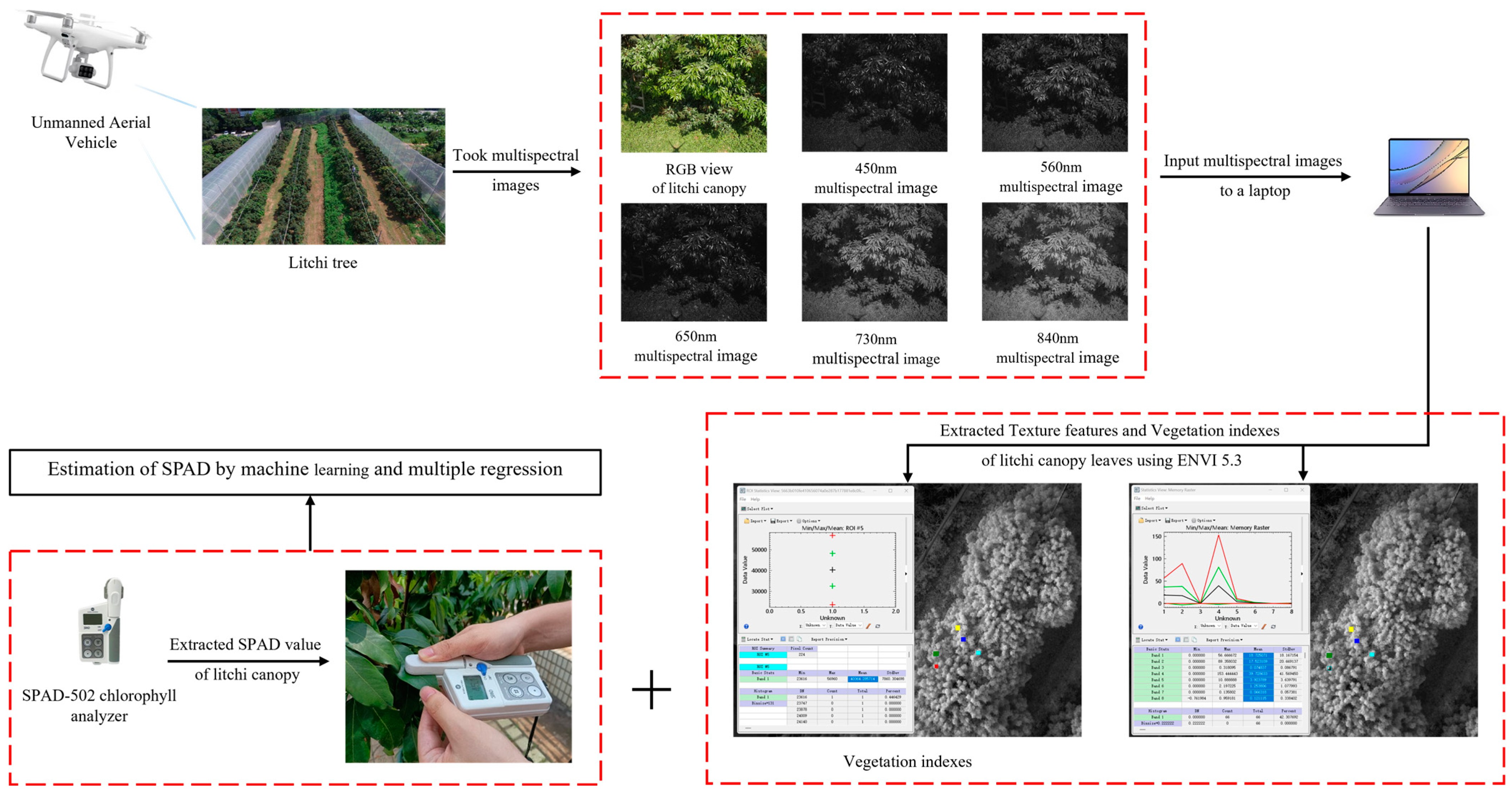
In this study, a DJI Phantom 4 UAV equipped with a multi-spectral camera served as the remote sensing image acquisition system. Simultaneously, a SPAD-502 chlorophyll analyzer was employed to collect ground-level SPAD values from the litchi canopy, establishing an open-ground integrated system for testing. The DJI Phantom 4 camera featured a 1/2.3-inch CMOS image sensor with 12 million effective pixels and a lens possessing an f/2.8 aperture, offering a 94° field of view. The parameters of the UAV multi-spectral camera are detailed in Table 1, and the schematic diagram of the data acquisition system is depicted in Figure 2. As illustrated in Figure 2, this study utilized the DJI Phantom 4 UAV equipped with a multispectral camera to capture multispectral images of litchi orchards’ canopies. These images were input into the computer and processed using ENVI software to extract vegetation indices and texture features. Combined with simultaneously collected ground-level SPAD values, an inversion model was constructed.
To mitigate the impact of the solar irradiation angle on the multi-spectral images, this study conducted the collection of multi-spectral images at noon during sunny weather. The specific testing procedure comprised the following steps: Step (1): Collection of multi-spectral images. Between 8 March and 15 October 2022, during periods characterized by clear skies and an absence of clouds, the UAV captured multi-spectral images from 11:00 to 13:00 [24]. This collection included 134 multi-spectral images of the litchi canopy during its fruit development period. A total of 132 multi-spectral images of the litchi canopy during the autumn shoot period were collected. Additionally, a calibration plate was captured daily to facilitate the calibration and correction of subsequent multi-spectral image data. Step (2): Collect litchi SPAD data. Concurrently with the acquisition of multi-spectral remote sensing images, the SPAD-502 chlorophyll instrument gathered SPAD data on the ground. This instrument gauged the absorption rate in the two wavelength segments of leaves to assess the relative content of chlorophyll. The SPAD value was determined as follows: At the central part of the leaf, avoiding the vein, three different locations were randomly selected for measurement. The average of these three measurements constituted the final SPAD value for that leaf. Across five regions, three litchi leaves were chosen from each region [25].

2.3. Spectral Reflectance Acquisition

Multi-spectral images of four different litchi varieties (Kwai flavor, glutinous rice paste, Xian Jinfeng, and Huai Zhi) were captured using multi-spectral cameras mounted on the UAV. The multi-spectral sensors employed in this experiment included red, green, blue, red-edge, and near-infrared spectral bands. Prior to UAV flight, route planning was executed based on the litchi distribution in the orchard. The UAV altitude was set at 25 m, the flight speed at 6.3 km/h, the shutter speed of the multi-spectral camera at 1/1000 s, sensitivity at 50, and the photographing interval at 1 s. The camera resolution was 1.3 CM/PX. Before entering the route, an image of the multi-spectral calibration plate was captured to calibrate the multi-spectral image information. In this study, yellow tags were affixed to every cluster of canopy leaves. During each measurement session, SPAD values of three leaves from the same canopy layer were simultaneously measured and then averaged. This average value was associated with the yellow tags observed on the multi-spectral image one by one. The Agisoft PhotoScan Professional software was employed to merge the visible and calibrated multi-spectral images obtained from the UAV. It also generated the corresponding high-definition digital orthophoto map (DOM). This DOM was input into the image processing software ENVI5.3, and the Di value of the corresponding band was extracted by dividing the region of interest (ROI) [26]. Then, the spectral reflectance Ri of each band was calculated according to Formula (1) [27].
R i = D i D b i R b i
In Formula (1), Ri—ground target reflectance in band i, Di—DN value at band i of ground target, Rbi—reflectivity of gray board in band i, Dbi—DN value of band i of gray board.

2.4. Selection and Calculation of Vegetation Indexes and Texture Features

In agriculture-related research, the vegetation index serves as a crucial indicator that reflects the status of crop growth, offering specific and valuable agricultural information [28]. In this experiment, 11 distinct vegetation indexes, including the red-edge chlorophyll index, modified secondary soil regulated vegetation index, and re-normalized vegetation index, were initially chosen. The corresponding calculation formulas for each index are provided in Appendix A.
Simultaneously, the ENVI5.3 software processed and gathered multi-spectral remote sensing images of litchi. It extracted eight texture features from the multi-spectral remote sensing images of the litchi canopy leaves for each band based on the gray scale co-occurrence matrix. These features encompassed mean, variance, homogeneity, contrast, dissimilarity, entropy, second moment, and correlation. Given that the experiment collected multi-spectral remote sensing images in the 450, 540, 650, 730, and 840 nm bands, with eight texture features extracted from each band, a total of 40 texture features were obtained from the five spectral bands.
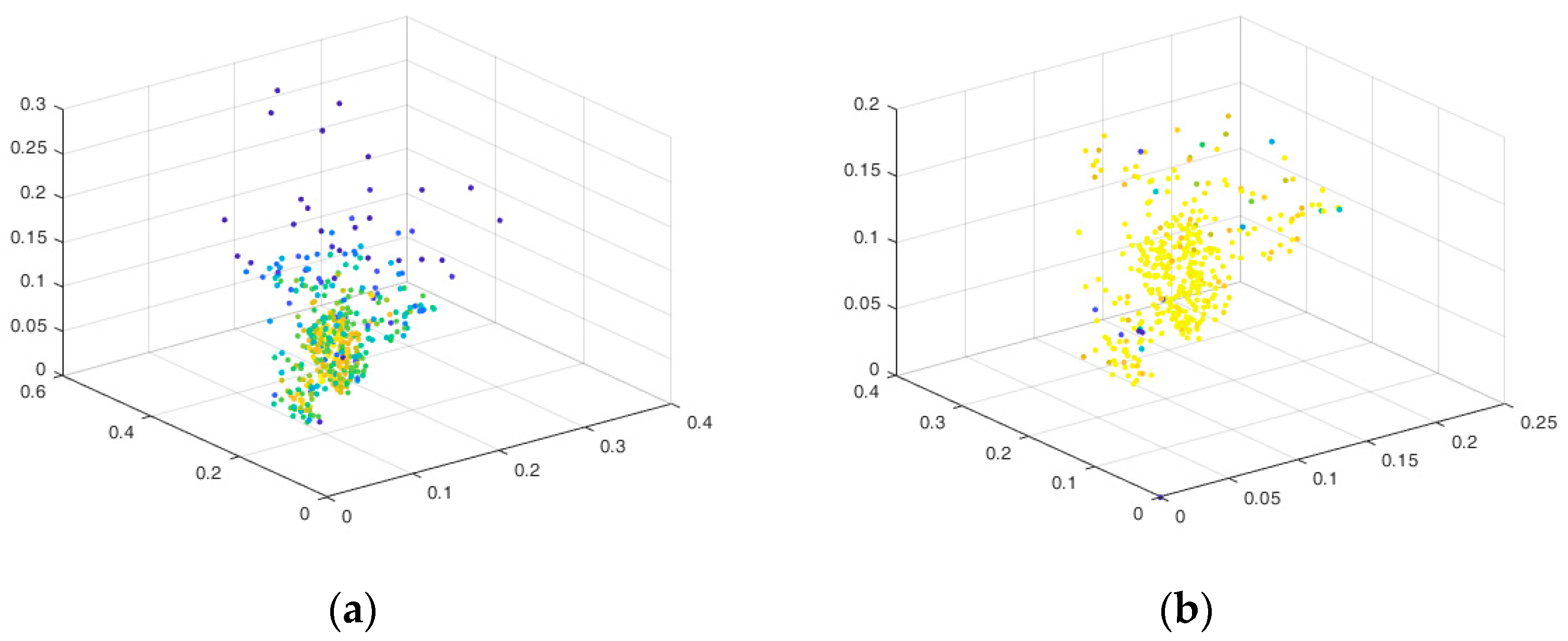
Following data collection, three datasets were compiled: vegetation indexes and the SPAD dataset, texture features and the SPAD dataset, and vegetation indexes combined with texture features and the SPAD dataset during the fruit growth period, resulting in 164 samples. For the litchi fruit growth period and autumn shoot period, 294 samples were acquired from the same three datasets. Each dataset underwent preprocessing, with the SVM algorithm utilized to identify and eliminate outliers. The distribution diagram in Figure 3 illustrates the dataset before and after screening. Figure 3a displays the initial data distribution, revealing both excessive centralization and discreteness. Post-screening, the data distribution demonstrated increased concentration, mitigating the discreteness. Consequently, 134 valid samples were retained for the litchi fruit growth period across the three datasets, and for the litchi fruit growth period and autumn shoot period, 266 groups of valid samples were secured.

2.5. Machine Learning Model

SVR, a widely employed machine learning method, operates on the principle of identifying an optimal classification plane to minimize structural risks. This method is characterized by its robust adaptability and straightforward structure, rendering it extensively utilized in regression analysis [29]. The main hyperparameters of this algorithm are penalty coefficient c and parameter gamma. If the value of c or gamma is too large, the model will be overfitted; if the value is too small, the model will be underfitted.
Beyond SVR, another commonly used machine learning method is random forest (RF), a statistical learning technique that has gained popularity among scholars due to its high accuracy, resistance to overfitting, and robust noise handling capabilities [30]. The primary hyperparameter of the algorithm is n_estimators, denoting the number of trees in the forest. Theoretically, a larger value is better, but it also increases computation time. The default setting is n_estimators = 50.
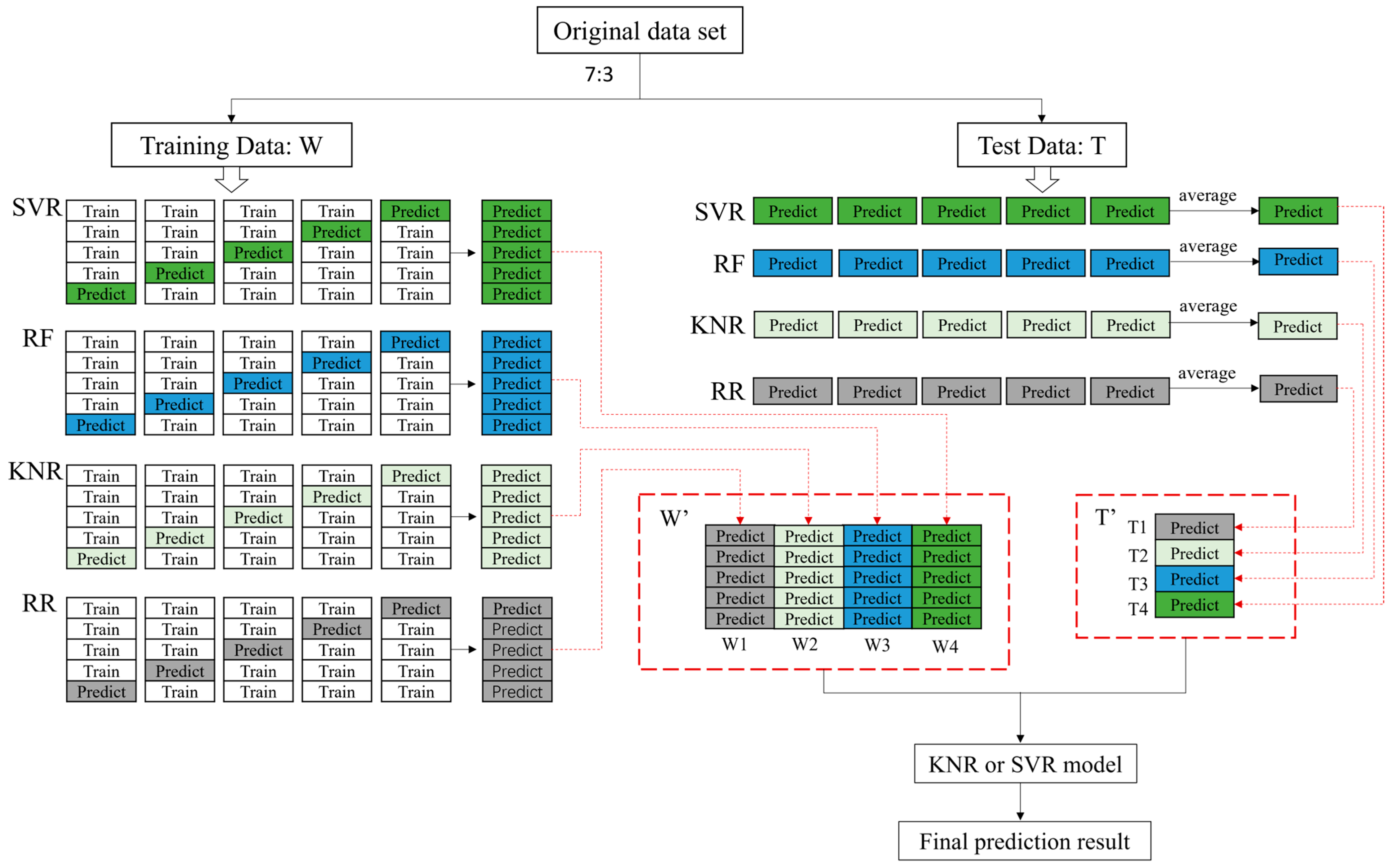
Currently, it is common to predict or infer plant phenotypic information using a single machine learning method. However, a single machine learning model often has a weak resistance to interference, making it necessary to combine multiple models to create a new model that enhances estimation accuracy. The ensemble learning method addresses the limitations of a single model. There are three general ensemble learning methods, one of which is the boosting algorithm that constructs robust learners sequentially between base learners. The second one is the bagging algorithm, which develops multiple independent models and then builds robust learners through selection or weighting. The bagging algorithm, proposed by Leo Breiman in 1996, is representative of parallel learning. In the parallel structure, each learner uses datasets generated by resampling, where each data sample has an equal probability of being sampled. This improves the reliability of the model. For regression problems, after training is completed, bagging typically adopts the arithmetic average method to average the predicted results of all models, obtaining the final results [31]. The third ensemble learning method is the stacking algorithm. It was first proposed by Wolpert in 1992 and combines boosting and bagging. It divides raw data into base learners according to certain rules, and the predicted results obtained after training each base learner are the output from the first-layer model. The output result is taken as the input of the second-layer model, and the meta-learner of the second-layer model is used for training to finally achieve the predicted result [32]. Specifically, training the stacking model consisted of three steps [33]. First, the dataset was divided and the base learner was determined. For the collected dataset A = { ( y n , x n ) , n = 1 , 2 , , N } , x n represented the feature vector of the NO. n sample and y n represented the predicted value corresponding to the NO. n sample. The sample dataset was divided into training set W and test set T by random sampling; the number of base learners was determined to be M and the number of meta-learners was determined to be 1. Second, the k-fold crossover operation was performed. Taking the first base learner as an example, W 1 was divided into k folds for training k times. In each training, 1 fold was left as the validation set, and the remaining folds were used as the training set for each training. This ensured that the validation set was different for each training, which was crucial for the high accuracy of the stacking algorithm. The predicted values obtained from each verification set in the kth training were stacked together and recorded as the new training set W 1 . Meanwhile, each training was predicted on the test set T . Therefore, after k times of training, the predicted results were averaged, and we used T 1 as the new test set. There were 4 base learners in this experiment, so new training sets W 1 , W 2 , W 3 , W 4 and new test sets T 1 , T 2 , T 3 , T 4 were obtained. The new training sets and the new test sets were stacked together to form the training set W and the test set T of the second layer. Third, the meta-learner was trained. By using W and T to train the selected meta-learner, the final prediction result was obtained. In this experiment, the dataset of stacking and bagging was divided into 5 folds and two layers of training were used. In fact, the number of layers of training and the number of meta-learners can be determined according to the needs [34].
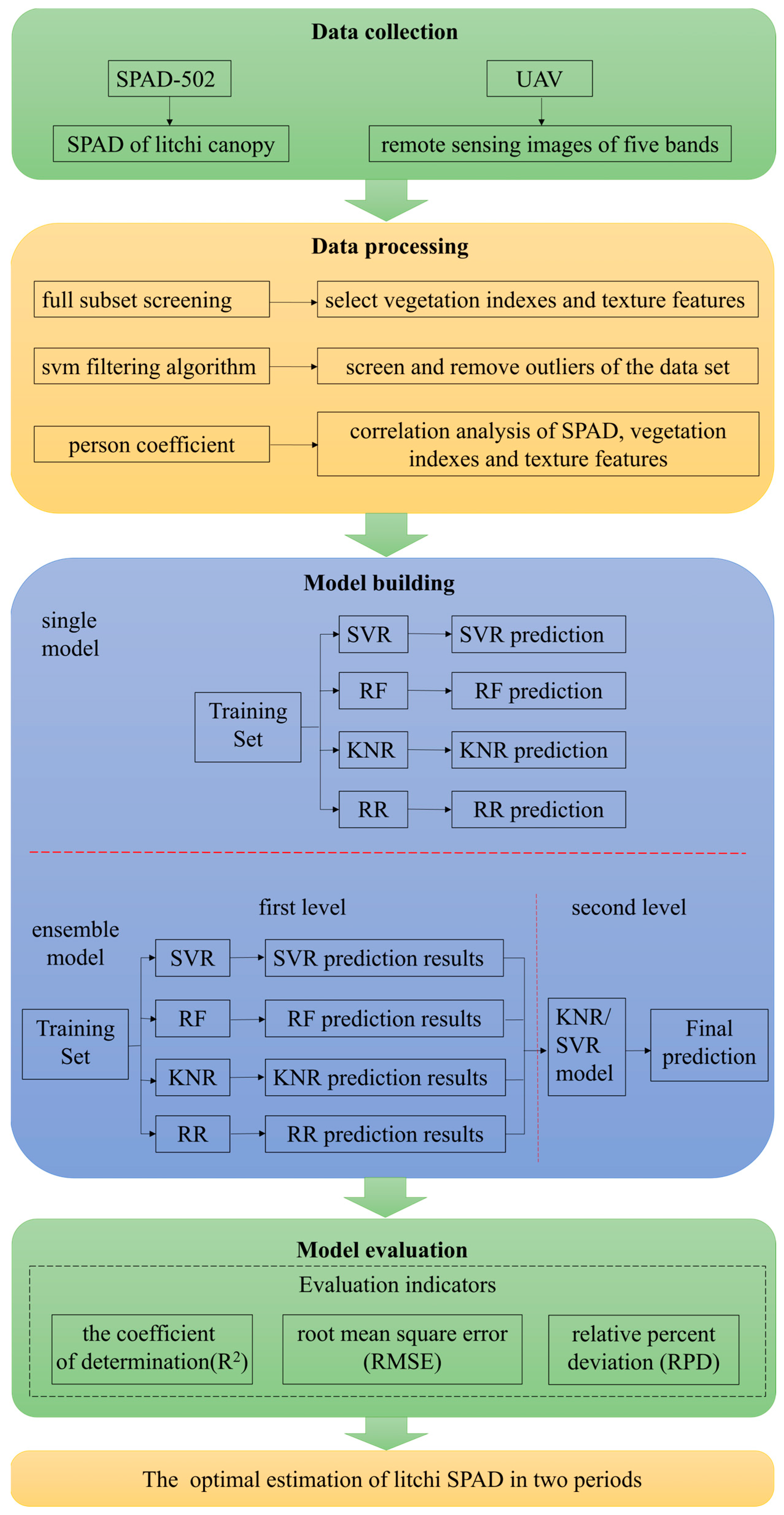
The structure of the stacking algorithm in this paper is illustrated in Figure 4. The study modeled and validated datasets under different combinations of independent variables in various litchi growth stages. It ensured a consistent 7:3 ratio of training sets to verification sets for each dataset, and an equal number of samples in each dataset under each period. Machine learning methods, including stacking, bagging, SVR, RF, KNR, and RR, were employed for modeling and analysis. The predicted values of each model were compared with the measured values to assess the performance of different models, with a specific focus on ensemble learning methods. The research flow chart is presented in Figure 5.

2.6. Verification Methods for Model Performance Indicators

The coefficient of determination (R2), root mean square error (RMSE), and relative percent deviation (RPD) were used to evaluate the prediction accuracy of the model. RMSE, R2, and RPD were used to compare the predicted value and the actual measured value of the model output, and the formula was
R 2 = i = 1 n ( x c a l x m e a n ) 2 ( y p r e d y m e a n ) 2 n i = 1 n ( x c a l x m e a n ) 2 i = 1 n ( y p r e d y m e a n ) 2
R M S E = i = 1 n ( y p r e d x c a l ) 2 n
R P D = S D R M S E ,
where xcal represents the actual measured value, xmean represents the mean value of the actual measured value, ypred represents the predicted value, ymean represents the mean value of the predicted value, and SD represents the standard deviation of the sample. The value range of R2 is 0 to 1, and the smaller the value of RMSE, the better. The RPD is divided into three levels: when the RPD is less than 1.4, the effect of the constructed regression model is weak; when the RPD is greater than or equal to 1.4 and less than 2, it indicates that the constructed regression prediction model has an average effect and can be used for rough estimation; when the RPD is greater than 2, it indicates that the constructed regression estimation model has a good effect and the estimation effect is ideal.

3. Results

3.1. SPAD Data Analysis

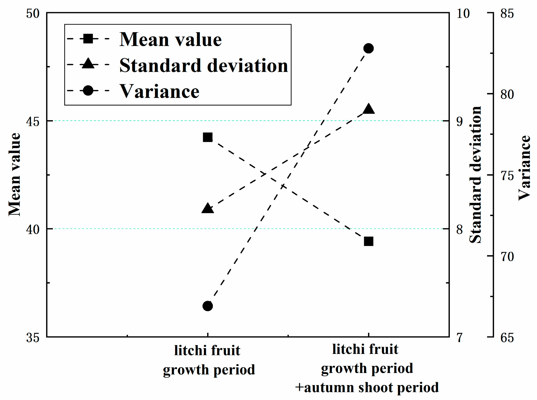
The measured data are depicted in Figure 6. In the litchi fruit growth period, the mean value, standard deviation, and variance of the measured 164 groups of original sample data were 44.237, 8.179, and 66.901, respectively. For the growth period and autumn shoot period combined, the mean value, standard deviation, and variance of 294 samples were 39.425, 9.099, and 82.792, respectively. The SPAD data concentration measured during the litchi fruit growth period exhibited better homogeneity. However, there was little difference between the two statistical datasets, making them suitable for modeling and verification.

3.2. Correlation Analysis of UAV Multi-Spectral Vegetation Indexes, Texture Features, and Litchi SPAD

Correlation analysis was conducted on the optimal combination of vegetation indexes and texture features with the measured SPAD values of litchi canopy leaves. The results are presented in Figure 7. In Figure 7a, during the growth and development of litchi fruit, only entropy (650 nm), moment (650 nm), and homogeneity (730 nm), along with the MCARI vegetation index, exhibited positive correlations with the SPAD values of litchi fruit. The Pearson coefficient of homogeneity (730 nm) was the highest at 0.217, indicating a strong positive correlation between homogeneity (730 nm) and litchi SPAD. Conversely, other vegetation indexes and texture features showed negative correlations with the SPAD values of litchi. The Pearson coefficients of the vegetation indexes MSAVI, OSAVI, RDVI, RVI2, and SIPI were higher at −0.531, −0.452, −0.356, −0.571, and −0.544, respectively. These results suggest that most vegetation indexes had a robust negative correlation with litchi SPAD.
Figure 7b illustrates the correlation analysis of vegetation indexes, texture features, and litchi SPAD during the fruit growth period + autumn shoot period. In Figure 7b, in addition to the positive correlation observed between DVI, MCARI, TCARI, and SPAD values, the remaining vegetation indexes and texture features exhibited negative correlations with the SPAD values. Notably, among the positive correlations, TCARI had the highest Pearson coefficient (0.305). Concerning the negatively correlated features with litchi SPAD, SIPI showed the highest absolute value of Pearson coefficient (−0.598). The Pearson coefficients of other negatively correlated vegetation indexes and texture features ranged from −0.037 to −0.598.

3.3. Model Fitting Performance Results

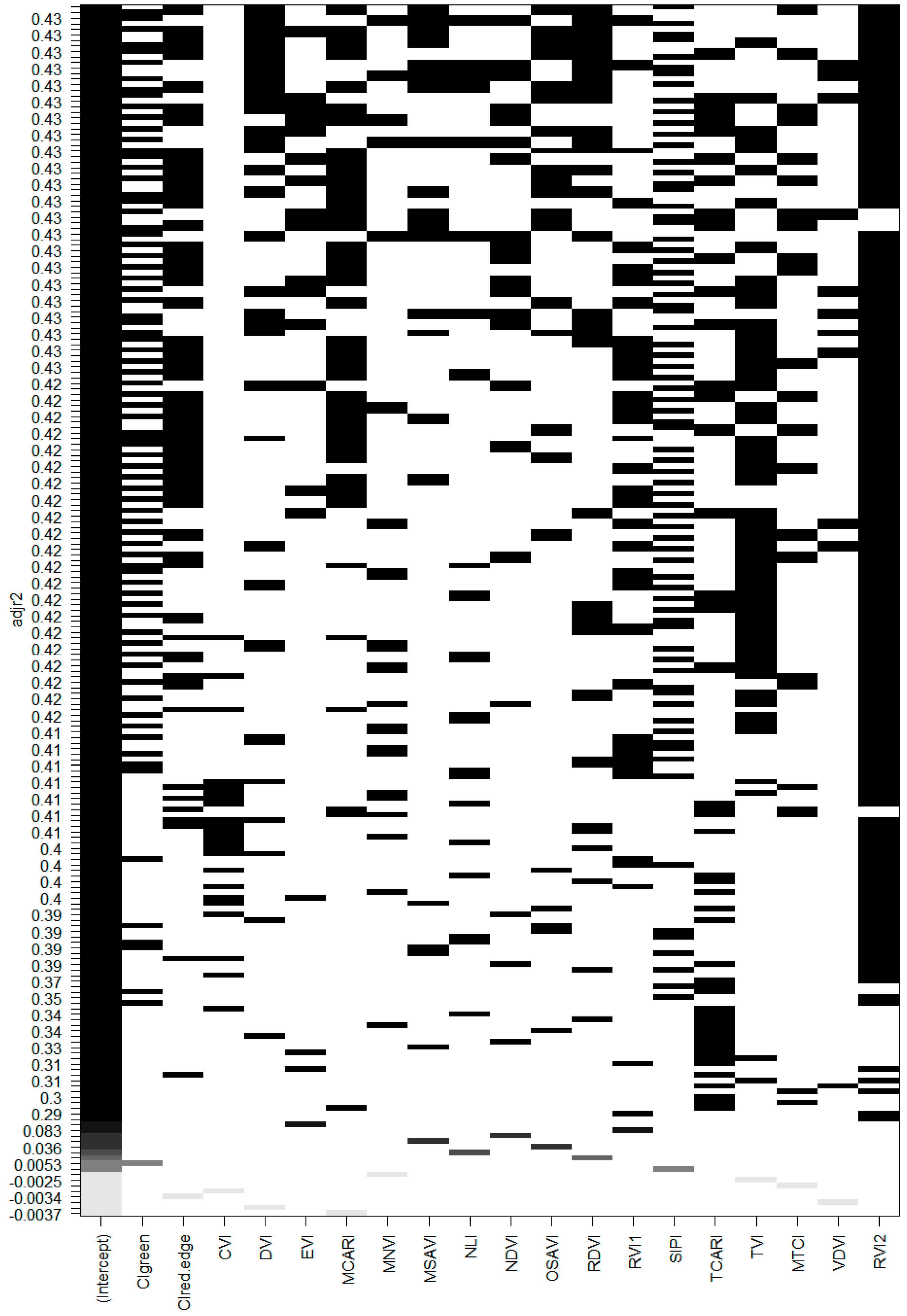
The full subset screening method involved attempting all possible combinations of independent variables. In this method, full subset regression was employed to perform fitting modeling. Full subset regression entails testing each conceivable combination of independent variables among all available variables, facilitating a least square fitting between these independent variables and the dependent variables [35]. The larger R2 of the model’s determination coefficient after fitting indicated that the combination of independent variables under the model was the optimal combination. For example, Figure 8 showed the selection of independent variable combinations by full subset screening method when vegetation indexes were used as independent variables in the growth period of litchi. It can be seen from Figure 3 that there were eight kinds of independent variable combinations with determination coefficients up to 0.43, and the second combination was found to have the best verification effect after experiment in this paper.
In this study, the spectral reflectance of the multi-spectral camera’s five bands (450, 560, 650, 730, and 840 nm) was computed. Various vegetation indexes were subsequently derived, as outlined in Table 2. Simultaneously, a full subset analysis was performed by integrating the 40 texture features from the five bands with the litchi SPAD. This process aimed to screen the optimal types and quantities of different independent variables, and the final results are presented in Table 2.

3.3.1. Estimation Model Based on Litchi Fruit Development Period

The dataset, after removing outliers, was partitioned into training and validation sets at a 7:3 ratio. The optimal combination of independent variables served as input, while the litchi canopy leaf SPAD acted as the output. The algorithms employed for estimating the litchi SPAD value included SVR, RF, KNR, RR, and stacking. The results of SPAD value estimation during the litchi fruit growth period are presented in Table 3.
Table 3 indicates that among the SPAD estimation models relying on the vegetation indexes of litchi fruit during the growth period, each model exhibited good stability, with determination coefficients (R2) exceeding 0.64. The most effective model was the stacking model, which amalgamated the SVR, RF, KNR, and RR models used in this experiment. Moreover, the SVR model was employed as a meta-learner for training, with the optimal training results achieved by setting superparameters store_train_meta_features = 3 and random_state = 6. The R2, RMSE, and RPD for the validation sets were 0.91, 2.8, and 2.4, respectively.
In the SPAD estimation model based on litchi fruit texture features during its growth period, the optimal model remained the stacking model, combining SVR, RF, KNR, and RR models. The KNR model was chosen as a meta-learner for training, with superparameters store_train_meta_features and random_state set at 7. The validation set’s R2, RMSE, and RPD for this model were 0.69, 4.6, and 1.4, respectively. Nevertheless, the estimation model based on texture features was not as effective as that based on vegetation indexes. The correlation analysis suggested that, whether positive or negative, the correlation between most texture features and SPAD was not as strong as that between vegetation indexes and SPAD. Therefore, the estimative ability of texture features for litchi SPAD was not as robust as that of vegetation indexes.
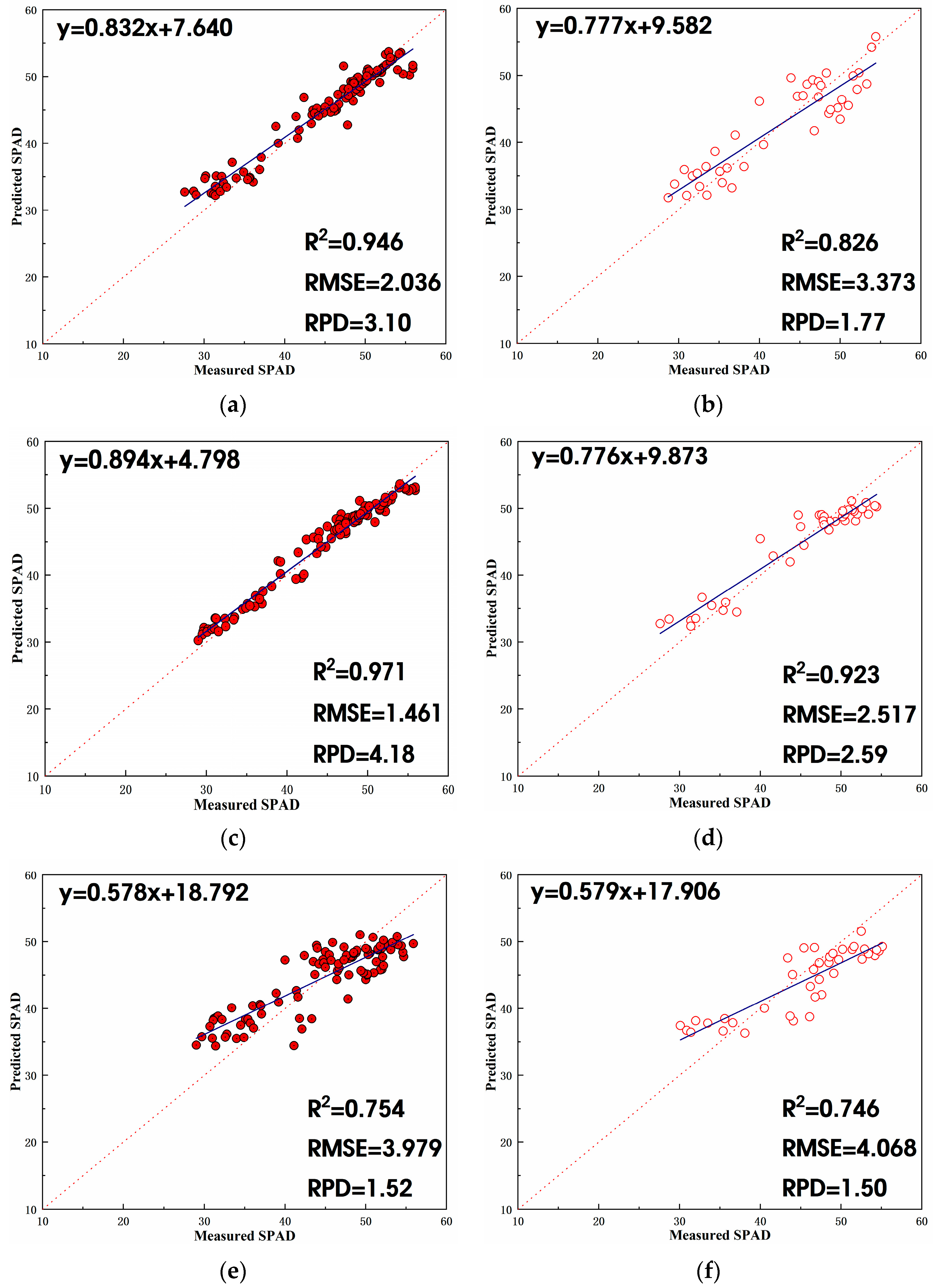
In the SPAD estimation model based on the vegetation indexes + texture features of litchi fruit during the growth period, the stability of each model was high, and the determination coefficient R2 for both the training set and the validation set reached 0.71 or above. Figure 9 illustrates the training and validation effects of the five models, indicating that the stacking model was optimal for estimating the SPAD of litchi. This model combined SVR, RF, KNR, and RR models, with SVR serving as a meta-learner, and the superparameters store_train_meta_features and random_state set at 3 and 6, respectively. The R2 of the training set was 0.98, the RMSE was 1.3, and the RPD was 4.7. The R2 of the validation set was 0.94, the RMSE was 2.4, and the RPD was 3.0. Even the weakest RR model achieved an R2 of 0.71 for the validation set. Comparing the estimation effect of the stacking model with the RR model, it is evident that the R2 of the validation set for the stacking model was 32.8% higher than that of the RR model, and the RMSE was 38.5% lower than that of the RR model. This underscores the advantages of the stacking learning method, particularly when dealing with numerous independent variables, as the stacking algorithm’s fitting effect surpasses that of a single machine learning method.
When scrutinizing each model, it becomes evident that among the three combinations of independent variables, the stacking model performed optimally, boasting the highest R2 and RPD values. This suggests that the stacking model exhibits strong reliability in estimating litchi SPAD. Moreover, its RMSE is nearly the lowest, aligning with the corresponding results of R2 and RPD. This implies that the stacking model maintains robust generalization ability in estimating litchi SPAD across different combinations of independent variables, showcasing a stable model estimation capability.

3.3.2. Estimation Model Based on Litchi Fruit Growth Period + Autumn Shoot Period

The dataset, after excluding outliers, was partitioned into training and validation sets at a 7:3 ratio. The optimal combination of independent variables was used as input, and the SPAD value of litchi canopy leaves was treated as the output. Various algorithms, including SVR, RF, KNR, RR, stacking, and bagging, were employed to estimate the SPAD value of litchi. The estimation modeling and validation results for the SPAD value of litchi fruit during its growth period and autumn shoot period are presented in Table 4.
From Table 4, it is evident that the ensemble learning model exhibited the most favorable training outcomes for litchi during the fruit growth period + autumn shoot period. The stacking model, combining SVR, RF, KNR, and RR, with SVR as the meta-learner, demonstrated superior performance. Setting superparameters store_train_meta_features to 6 and random_state to 3, the stacking model achieved an R2 of 0.91, an RMSE of 2.8, and an RPD of 2.4 in the validation set. In comparison with the less effective RF model, the stacking model improved the R2 and RPD of the validation set by 24.7% and 60.0%, respectively, while reducing RMSE by 36.4%.
The overall performance of the estimation models based on texture features was suboptimal, with low R2 values in the validation sets for all models. However, the bagging learning method showed promise. Using SVR as the base learner and setting random_state to 3, the bagging model achieved the optimal R2 of 0.42 in the validation set. Taking into account the fitting performance of all models, it was observed that estimating the SPAD value of litchi based on the fruit growth period and autumn shoot period was not effective.
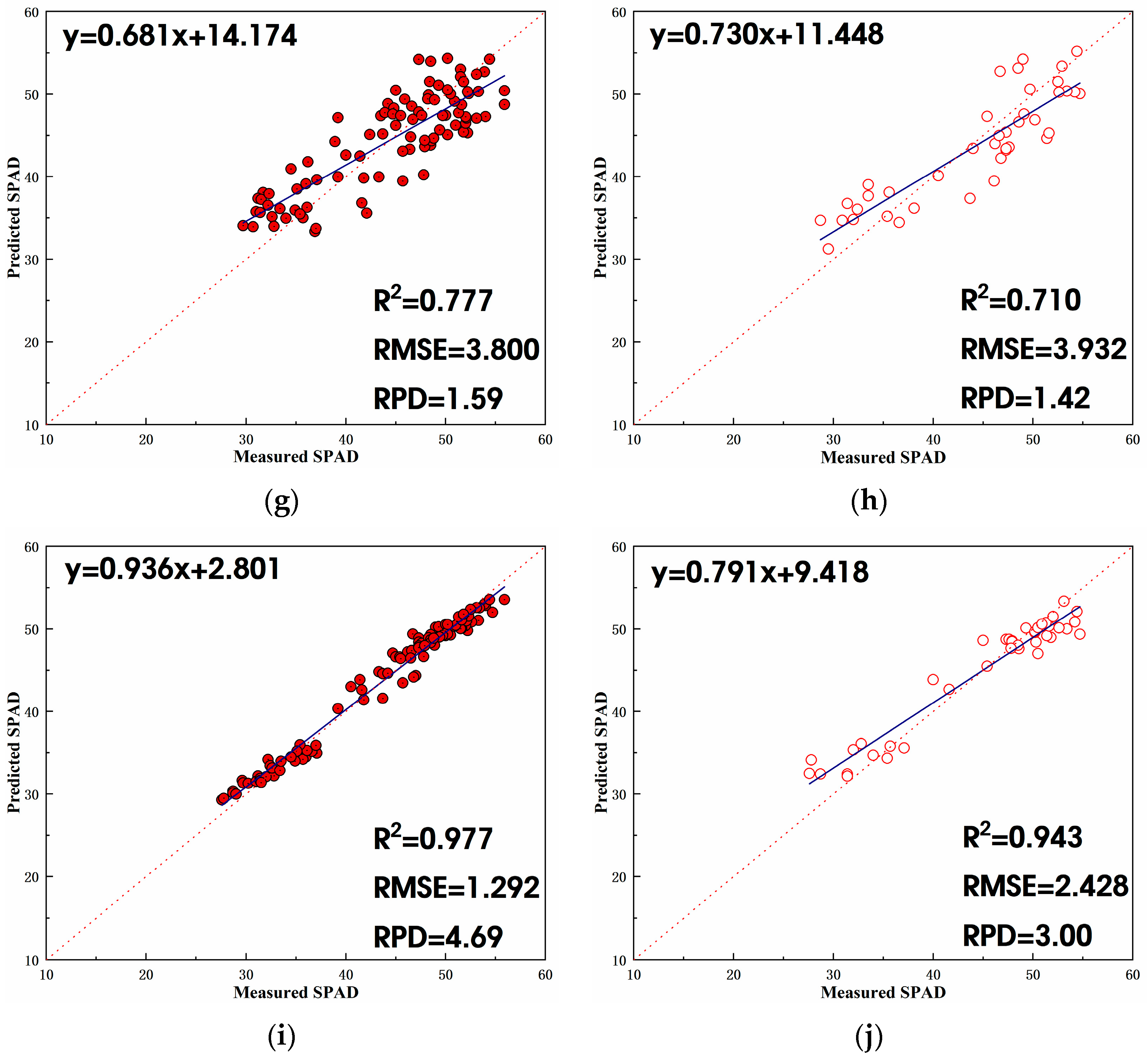
The estimation models based on vegetation indexes + texture features generally demonstrated good effects. In Figure 10, it can be observed that even the RR model with the least favorable fitting effect had a relatively high R2 value of 0.64 in the validation set. The optimal estimating model remained the stacking model, which combined SVR, RF, KNR, and RR. SVR was used as the meta-learner, with the superparameters store_train_meta_features and random_state set as 6 and 3, respectively. The R2, RMSE, and RPD of the training set were 0.95, 2.1, and 3.2, respectively. The R2 of the validation set was 0.84, the RMSE was 3.9, and the RPD was 1.9. Compared with the weakest RR model, the R2 and RPD of the validation set of the stacking model increased by 31.3% and 46.2%, respectively, and the RMSE decreased by 27.8%. Taking all factors into consideration, the stacking model was deemed the optimal estimation model based on vegetation indexes + texture features in the litchi fruit growth period + autumn shoot period.
Observing the models in the three combinations of independent variables, it is notable that both the stacking model and the bagging model performed optimally, further affirming the effectiveness of the ensemble learning method, particularly when vegetation indexes were employed as independent variables. The R2 of the validation set for the stacking model (0.91) was 24.7% higher than that of the optimal RF model in the single model (0.73), indicating that the estimating ability of the stacking model was more reliable than that of the single model. Compared to Table 3, it can be observed that in Table 4, there are fewer cases where the RPD is greater than 2. Firstly, it should be pointed out that the training set’s performance is bound to be better than that of the validation set. Therefore, whether in Table 3 or Table 4, the instances where the RPD of the training set is greater than 2 are always more than those of the validation set. Secondly, Table 4 presents the modeling results for the combined stages of autumn shoot and fruit growth, whereas Table 3 specifically displays the fruit growth period. Due to the smaller amount of data in Table 3 compared to Table 4, and considering that a larger dataset often implies the need to consider more factors, leading to greater uncertainty in modeling, the phenomenon of a better RPD in Table 3 appears natural and predicted.

4. Discussion

The SPAD values of litchi canopy leaves were collected synchronously based on UAV multi-spectrum in this study. The data extraction involved obtaining five-band spectral reflectance, vegetation index, and texture features from the collected multi-spectral remote sensing images. The optimal independent variable combination was determined through the full subset screening method. Three datasets were constructed for the litchi fruit growth period and three for the litchi fruit growth period + autumn shoot period. A correlation analysis was conducted between vegetation indexes, texture features, and SPAD values for each dataset, verifying the relatively ideal nature of the independent variable combination obtained by the full subset screening method. In the litchi fruit growth period, only entropy (650 nm), moment (650 nm), homogeneity (730 nm), and the MCARI were positively correlated with the litchi SPAD value. Conversely, other vegetation indexes and texture features were negatively correlated with the litchi SPAD value. The strongest negative correlation with SPAD in the litchi fruit growth period was observed for the vegetation index RVI2, with a Pearson coefficient of −0.571, followed by the vegetation index SIPI, with a Pearson coefficient of −0.544. Additionally, in the litchi fruit growth period and autumn shoot period, in addition to the positive correlation between the three vegetation indexes (DVI, MCARI, TCARI) and the SPAD value, other vegetation indexes and texture features were negatively correlated with the SPAD value. The strongest negative correlation with SPAD in this combined period was observed for the vegetation index SIPI, with a Pearson coefficient of −0.598.
The study indicates that, for both the litchi fruit growth period and the combined litchi fruit growth period + autumn shoot period, the model employing a combination of vegetation indexes and texture features as independent variables provided the most accurate SPAD estimation. It was followed by the model using only vegetation indexes, while the model using only texture features performed less effectively. These results suggest that the combination of vegetation indexes and texture features yields the best SPAD estimation for litchi. Vegetation indexes alone demonstrated a strong estimating ability, and while texture features showed some potential, predicting litchi SPAD solely based on texture features was not optimal. Future research directions could involve a deeper analysis of the mechanisms behind texture features and exploring additional variable combinations. In subsequent studies, expanding the range of included vegetation indexes, optimizing the selection of these indexes, and examining the model’s adaptability could be beneficial. Additionally, litchi SPAD may be influenced by various factors such as meteorological conditions and moisture levels. Thus, future research might consider more comprehensive data acquisition systems in litchi orchards, conducting long-term experiments to measure diverse field data. This approach could further validate the litchi SPAD value estimation model proposed in this study.
The stacking algorithm has been widely used in soil evapotranspiration prediction, soil moisture estimation, and so on [36,37]. Compared with other scholars’ studies, this experiment proposed the application of an ensemble learning method to estimate litchi SPAD. It was found that in the models with different combinations of independent variables, the estimation results of the ensemble learning models were all better than those of single models. In this experiment, the ensemble learning model constructed with the stacking algorithm and bagging algorithm achieved good estimation effects. In particular, the stacking algorithm could be applied to many different datasets in this experiment and achieve optimal estimation results, indicating its strong generalization ability. The stacking algorithm, as an ensemble learning method, has been mainly applied in situations with a large amount of data and multiple feature dimensions. The stacking algorithm also allows many features to be weak because it can combine a part of the weak features into a strong feature. For example, Tao et al. [37] used the stacking algorithm to predict soil moisture in grape-growing areas. At the first layer, this study ensembled tree model-based algorithms consisting of RF, GBDT, and CatBoost, and at the second layer, LR was used as meta-learner. Finally, it was found that the R2 of the validation set of the ensembled model could reach 0.7504. This study found that the ensemble learning model was much better than the original single model, but there was also a shortcoming, that is, the first-layer-based learning devices had a poor fitting effect, which limited the improvement of the fitting effect of the ensemble learning model to a certain extent. In addition, the differences between the first layer of base learning devices were reflected in the difference in the focus of data mining between single models. For example, the KNR algorithm paid more attention to the distance relationship between samples, and the RF algorithm paid more attention to the sample impurity changes before and after feature splitting. Moreover, the effect of each base learning device should be ideal enough. This will make the ensemble learning model more stable. Therefore, in this experiment, algorithms such as SVR, RF, KNR, and RR were combined into a model using the stacking algorithm. The advantages of each single model were taken into account while the fitting effect of most of the single models was already good. Most accuracy indicators of the various models in the final estimation results were better than that of a single model. In further research, it will be possible to optimize the selection of the stacking algorithm and optimize the base learners to further improve the estimation effect of the ensemble learning algorithms. In addition, further long-term research must be conducted on the relationship between litchi SPAD and yield and quality to improve the model in this paper for litchi yield estimation. It will also be necessary to monitor the whole growth cycle of litchi to form a more systematic experience, so as to provide greater theoretical support for the field management of litchi.

5. Conclusions

In this study, litchi trees served as the focal point of investigation. Remote sensing images of litchi canopy leaves were acquired using a meticulously controlled UAV equipped with a multi-spectral camera. Subsequently, spectral reflectance, vegetation index, and texture features of the litchi canopy leaves were extracted from these images. Concurrently, SPAD values of the litchi canopy leaves were meticulously measured on the ground using a chlorophyll meter. Employing vegetation index, texture features, and a combination of both as independent variables, the support vector regression (SVR), random forest (RF), k-nearest neighbors (KNR), and ridge regression (RR) models were deployed to estimate the SPAD values of litchi canopy leaves. The main research conclusions of the experiment were as follows:
(1)
For the litchi fruit growth period, three combinations of independent variables were investigated in this study: vegetation index, texture features, and vegetation index + texture features. Overall, the combination of vegetation index + texture features as independent variables exhibited the most effective estimation, followed by vegetation index alone and then texture features alone. In the SPAD estimation model developed in this study based on vegetation index + texture features during the fruit growth period, the stacking model demonstrated the highest R2 in the validation set, reaching 0.94. Following closely was the RF model with an R2 of 0.92. The stacking model also exhibited the lowest RMSE in the validation set, at 2.4, compared to 2.5 for the RF model. Additionally, the RPD of the validation set for the stacking model was the highest at 3.0, followed by 2.6 for the RF model. In summary, the stacking model proved to be the optimal choice for estimating the SPAD value of litchi fruit during its growth period based on vegetation index + texture features, followed by the RF model.
(2)
For the litchi fruit growth period + autumn shoot period, three combinations of independent variables were considered in this study: vegetation index, texture features, and vegetation index + texture features. Overall, the combination of vegetation index + texture features as independent variables demonstrated the most effective estimation, followed by vegetation index alone and then texture features alone. In the SPAD estimation model developed in this study based on vegetation index + texture features during the litchi fruit growth period + autumn shoot period, the stacking model exhibited the highest R2 in the validation set, reaching 0.84. Following closely was the RF model with an R2 of 0.81. The stacking model and RF model share the same lowest validation set RMSE, which is 3.9. The stacking model also showed the highest validation set RPD at 1.9, followed by 1.7 for the RF model. In summary, the stacking model was identified as the optimal choice for estimating the SPAD value of litchi fruit during its growth period + autumn shoot period based on vegetation index + texture features, followed by the RF model.

Author Contributions

Conceptualization, J.X. and J.W.; methodology, J.X. and J.W.; software, J.W.; validation, J.X. and J.W.; formal analysis, Y.C. and P.G.; investigation, J.X. and J.W.; resources, J.X. and J.W.; data curation, H.Y., S.C. and H.M.; writing—original draft preparation, J.X. and J.W.; writing—review and editing, J.X. and D.S.; visualization, J.X. and J.W.; supervision, J.S. and J.L.; project administration, W.W. and J.L. All authors have read and agreed to the published version of the manuscript.

Funding

This research was funded by the Co-constructing Cooperative Project on Agricultural Sci-tech of New Rural Development Research Institute of South China Agricultural University (No. 2021XNYNYKJHZGJ032). It was also partly supported by the China Agriculture Research System of MOF and MARA, China (No. CARS-32-11); the Guangdong Provincial Special Fund for Modern Agriculture Industry Technology Innovation Teams, China (No. 2023KJ108); the Key-Area Research and Development Program of Guangdong Province (No. 2023B0202090001); the Guangdong Science and Technology Innovation Cultivation Special Fund Project for College Students (“Climbing Program” Special Fund), China (No. pdjh2023a0074); and the Innovation and Entrepreneurship Training Program for College Students (202310564010).

Data Availability Statement

The data presented in this study are available on request from the corresponding author. The data are not publicly available due to the privacy policy of the organization.

Acknowledgments

The authors would like to thank the College of Horticulture, South China Agricultural University, for the support of the experimental litchi orchard. In addition, we would like to thank everyone who participated in this study.

Conflicts of Interest

The authors declare no conflict of interest.

Appendix A

Table A1. Summary of vegetation indexes.
Vegetation IndexCalculation FormulaReference
Chlorophyll Index of Red Edge, CIred Edge C I r e d   e d g e = N I R / R E 1 [38]
Modified Soil-Adjusted Vegetation Index, MSAVI M S A V I = 0.5 ( 2 N I R + 1 ) ( 2 N I R + 1 ) 2 8 ( N I R R ) [39]
Renormalized Vegetation Index, RDVI R D V I = ( N I R R ) / N I R + R [40]
Structure Insensitive Pigment Index, SIPI S I P I = ( N I R B ) / ( N I R + B ) [41]
Difference Vegetation Index, DVI D V I = N I R R [42]
Modified Chlorophyll Absorption Ratio Index, MCARI M C A R I = ( R E R 0.2 ( R E G ) ) R E / R [39]
Optimized Soil and Adjusted Vegetation Index, OSAVI O S A V I = 1.16 N I R R / N I R + R + 0.16 [43]
MERIS Terrestrial Chlorophyll Index, MTCI M T C I = ( N I R - R E ) / ( R E - R ) [44]
Ratio Vegetation Index 1, RVI1 R V I 1 = N I R / G [45]
Transformed Chlorophyll Absorption Reflectance Index, TCARI T C A R I = 3 ( R E R ) 0.2 ( R E G ) ( R E / R ) [46]
Non-Linear Index, NLI N L I = ( N I R 2 R ) / ( N I R 2 + R ) [47]
Note: B, G, R, RE, and NIR represent the spectral reflectance of the blue, green, red, red-edge, and near-infrared bands, respectively.

References

  1. Xie, J.; Peng, J.; Wang, J.; Chen, B.; Jing, T.; Sun, D.; Gao, P.; Wang, W.; Lu, J.; Yetan, R.; et al. Litchi Detection in a Complex Natural Environment Using the YOLOv5-Litchi Model. Agronomy 2022, 12, 3054. [Google Scholar] [CrossRef]
  2. Kuang, L.; Wang, Z.; Cheng, Y.; Li, Y.; Li, H.; Zhang, J.; Shen, Y.; Li, J.; Xu, G. Residue Levels and Risk Assessment of Pesticides in Litchi and Longan of China. J. Food Compos. Anal. 2023, 115, 104921. [Google Scholar] [CrossRef]
  3. Xiong, Z.; Wang, L.; Zhao, Y.; Lan, Y. Precision Detection of Dense Litchi Fruit in UAV Images Based on Improved YOLOv5 Model. Remote Sens. 2023, 15, 4017. [Google Scholar] [CrossRef]
  4. Liu, B.; Xue, W.; Guo, Z.; Liu, S.; Zhu, Q.; Pang, X.; Zhang, Z.; Fang, F. Water Loss and Pericarp Browning of Litchi (Litchi chinensis) and Longan (Dimocarpus longan) Fruit Maintain Seed Vigor. Sci. Hortic. 2021, 290, 110519. [Google Scholar] [CrossRef]
  5. Su, Z.; Liu, L.; Li, Y.; Chen, H. Predicting Flower Induction of Litchi (Litchi chinensis Sonn.) with Machine Learning Techniques. Comput. Electron. Agric. 2023, 205, 107572. [Google Scholar] [CrossRef]
  6. Fu, P.; Meacham-Hensold, K.; Siebers, M.H.; Bernacchi, C.J. The Inverse Relationship between Solar-Induced Fluorescence Yield and Photosynthetic Capacity: Benefits for Field Phenotyping. J. Exp. Bot. 2021, 72, 1295–1306. [Google Scholar] [CrossRef]
  7. Liu, P.; Huang, J.; Cai, Z.; Chen, H.; Huang, X.; Yang, S.; Su, Z.; Azam, M.; Chen, H.; Shen, J. Influence of Girdling on Growth of Litchi (Litchi chinensis) Roots during Cold-Dependent Floral Induction. Sci. Hortic. 2022, 297, 110928. [Google Scholar] [CrossRef]
  8. Fu, X.-Y.; Mo, W.-P.; Zhang, J.-Y.; Zhou, L.-Y.; Wang, H.-C.; Huang, X.-M. Shoot Growth Pattern and Quantifying Flush Maturity with SPAD Value in Litchi (Litchi chinensis Sonn.). Sci. Hortic. 2014, 174, 29–35. [Google Scholar] [CrossRef]
  9. Li, J.; Wijewardane, N.K.; Ge, Y.; Shi, Y. Improved Chlorophyll and Water Content Estimations at Leaf Level with a Hybrid Radiative Transfer and Machine Learning Model. Comput. Electron. Agric. 2023, 206, 107669. [Google Scholar] [CrossRef]
  10. Hassanijalilian, O.; Igathinathane, C.; Doetkott, C.; Bajwa, S.; Nowatzki, J.; Haji Esmaeili, S.A. Chlorophyll Estimation in Soybean Leaves Infield with Smartphone Digital Imaging and Machine Learning. Comput. Electron. Agric. 2020, 174, 105433. [Google Scholar] [CrossRef]
  11. Teshome, F.T.; Bayabil, H.K.; Hoogenboom, G.; Schaffer, B.; Singh, A.; Ampatzidis, Y. Unmanned Aerial Vehicle (UAV) Imaging and Machine Learning Applications for Plant Phenotyping. Comput. Electron. Agric. 2023, 212, 108064. [Google Scholar] [CrossRef]
  12. Yang, Y.; Wei, X.; Wang, J.; Zhou, G.; Wang, J.; Jiang, Z.; Zhao, J.; Ren, Y. Prediction of Seedling Oilseed Rape Crop Phenotype by Drone-Derived Multimodal Data. Remote Sens. 2023, 15, 3951. [Google Scholar] [CrossRef]
  13. Yu, T.; Zhou, J.; Fan, J.; Wang, Y.; Zhang, Z. Potato Leaf Area Index Estimation Using Multi-Sensor Unmanned Aerial Vehicle (UAV) Imagery and Machine Learning. Remote Sens. 2023, 15, 4108. [Google Scholar] [CrossRef]
  14. Jiang, J.; Zhang, Z.; Cao, Q.; Liang, Y.; Krienke, B.; Tian, Y.; Zhu, Y.; Cao, W.; Liu, X. Use of an Active Canopy Sensor Mounted on an Unmanned Aerial Vehicle to Monitor the Growth and Nitrogen Status of Winter Wheat. Remote Sens. 2020, 12, 3684. [Google Scholar] [CrossRef]
  15. Wan, L.; Zhu, J.; Du, X.; Zhang, J.; Han, X.; Zhou, W.; Li, X.; Liu, J.; Liang, F.; He, Y.; et al. A Model for Phenotyping Crop Fractional Vegetation Cover Using Imagery from Unmanned Aerial Vehicles. J. Exp. Bot. 2021, 72, 4691–4707. [Google Scholar] [CrossRef]
  16. Vélez, S.; Ariza-Sentís, M.; Valente, J. Mapping the Spatial Variability of Botrytis Bunch Rot Risk in Vineyards Using UAV Multispectral Imagery. Eur. J. Agron. 2023, 142, 126691. [Google Scholar] [CrossRef]
  17. Jiang, J.; Atkinson, P.M.; Zhang, J.; Lu, R.; Zhou, Y.; Cao, Q.; Tian, Y.; Zhu, Y.; Cao, W.; Liu, X. Combining Fixed-Wing UAV Multispectral Imagery and Machine Learning to Diagnose Winter Wheat Nitrogen Status at the Farm Scale. Eur. J. Agron. 2022, 138, 126537. [Google Scholar] [CrossRef]
  18. Huang, Y.; Ma, Q.; Wu, X.; Li, H.; Xu, K.; Ji, G.; Qian, F.; Li, L.; Huang, Q.; Long, Y.; et al. Estimation of Chlorophyll Content in Brassica Napus Based on Unmanned Aerial Vehicle Images. Oil Crop Sci. 2022, 7, 149–155. [Google Scholar] [CrossRef]
  19. Poudyal, C.; Sandhu, H.; Ampatzidis, Y.; Odero, D.C.; Arbelo, O.C.; Cherry, R.H.; Costa, L.F. Prediction of Morpho-Physiological Traits in Sugarcane Using Aerial Imagery and Machine Learning. Smart Agric. Technol. 2023, 3, 100104. [Google Scholar] [CrossRef]
  20. Zhang, L.; Han, W.; Niu, Y.; Chávez, J.L.; Shao, G.; Zhang, H. Evaluating the Sensitivity of Water Stressed Maize Chlorophyll and Structure Based on UAV Derived Vegetation Indices. Comput. Electron. Agric. 2021, 185, 106174. [Google Scholar] [CrossRef]
  21. Shen, L.; Gao, M.; Yan, J.; Wang, Q.; Shen, H. Winter Wheat SPAD Value Inversion Based on Multiple Pretreatment Methods. Remote Sens. 2022, 14, 4660. [Google Scholar] [CrossRef]
  22. Fei, S.; Chen, Z.; Li, L.; Ma, Y.; Xiao, Y. Bayesian Model Averaging to Improve the Yield Prediction in Wheat Breeding Trials. Agric. For. Meteorol. 2023, 328, 109237. [Google Scholar] [CrossRef]
  23. Li, Q.; Xu, S.; Zhuang, J.; Liu, J.; Zhou, Y.; Zhang, Z. Ensemble Learning Prediction of Soybean Yields in China Based on Meteorological Data. J. Integr. Agric. 2023, 22, 1909–1927. [Google Scholar] [CrossRef]
  24. Shao, G.; Han, W.; Zhang, H.; Zhang, L.; Wang, Y.; Zhang, Y. Prediction of Maize Crop Coefficient from UAV Multisensor Remote Sensing Using Machine Learning Methods. Agric. Water Manag. 2023, 276, 108064. [Google Scholar] [CrossRef]
  25. Wang, H.; Huo, Z.; Zhou, G.; Liao, Q.; Feng, H.; Wu, L. Estimating Leaf SPAD Values of Freeze-Damaged Winter Wheat Using Continuous Wavelet Analysis. Plant Physiol. Biochem. 2016, 98, 39–45. [Google Scholar] [CrossRef]
  26. Johansen, K.; Raharjo, T.; McCabe, M. Using Multi-Spectral UAV Imagery to Extract Tree Crop Structural Properties and Assess Pruning Effects. Remote Sens. 2018, 10, 854. [Google Scholar] [CrossRef]
  27. Xie, J.; Chen, Y.; Yu, Z.; Wang, J.; Liang, G.; Gao, P.; Sun, D.; Wang, W.; Shu, Z.; Yin, D.; et al. Estimating Stomatal Conductance of Citrus under Water Stress Based on Multispectral Imagery and Machine Learning Methods. Front. Plant Sci. 2023, 14, 1054587. [Google Scholar] [CrossRef]
  28. Islam, M.D.; Di, L.; Qamer, F.M.; Shrestha, S.; Guo, L.; Lin, L.; Mayer, T.J.; Phalke, A.R. Rapid Rice Yield Estimation Using Integrated Remote Sensing and Meteorological Data and Machine Learning. Remote Sens. 2023, 15, 2374. [Google Scholar] [CrossRef]
  29. Wang, Q.; Che, Y.; Shao, K.; Zhu, J.; Wang, R.; Sui, Y.; Guo, Y.; Li, B.; Meng, L.; Ma, Y. Estimation of Sugar Content in Sugar Beet Root Based on UAV Multi-Sensor Data. Comput. Electron. Agric. 2022, 203, 107433. [Google Scholar] [CrossRef]
  30. Wang, N.; Guo, Y.; Wei, X.; Zhou, M.; Wang, H.; Bai, Y. UAV-Based Remote Sensing Using Visible and Multispectral Indices for the Estimation of Vegetation Cover in an Oasis of a Desert. Ecol. Indic. 2022, 141, 109155. [Google Scholar] [CrossRef]
  31. Nasir Amin, M.; Iftikhar, B.; Khan, K.; Faisal Javed, M.; Mohammad AbuArab, A.; Faisal Rehman, M. Prediction Model for Rice Husk Ash Concrete Using AI Approach: Boosting and Bagging Algorithms. Structures 2023, 50, 745–757. [Google Scholar] [CrossRef]
  32. Das, B.; Rathore, P.; Roy, D.; Chakraborty, D.; Jatav, R.S.; Sethi, D.; Kumar, P. Comparison of Bagging, Boosting and Stacking Algorithms for Surface Soil Moisture Mapping Using Optical-Thermal-Microwave Remote Sensing Synergies. CATENA 2022, 217, 106485. [Google Scholar] [CrossRef]
  33. Liu, G.; Zhang, X.; Liu, Z. State of Health Estimation of Power Batteries Based on Multi-Feature Fusion Models Using Stacking Algorithm. Energy 2022, 259, 124851. [Google Scholar] [CrossRef]
  34. Ouyang, Z.; Zhou, C.; Xie, J.; Zhu, J.; Zhang, G.; Ao, M. SRTM DEM Correction Using Ensemble Machine Learning Algorithm. Remote Sens. 2023, 15, 3946. [Google Scholar] [CrossRef]
  35. Qiu, Y. Complete Subset Least Squares Support Vector Regression. Econ. Lett. 2021, 200, 109737. [Google Scholar] [CrossRef]
  36. Martín, J.; Sáez, J.A.; Corchado, E. On the Suitability of Stacking-Based Ensembles in Smart Agriculture for Evapotranspiration Prediction. Appl. Soft Comput. 2021, 108, 107509. [Google Scholar] [CrossRef]
  37. Tao, S.; Zhang, X.; Feng, R.; Qi, W.; Wang, Y.; Shrestha, B. Retrieving Soil Moisture from Grape Growing Areas Using Multi-Feature and Stacking-Based Ensemble Learning Modeling. Comput. Electron. Agric. 2023, 204, 107537. [Google Scholar] [CrossRef]
  38. Gitelson, A.A.; Gritz†, Y.; Merzlyak, M.N. Relationships between Leaf Chlorophyll Content and Spectral Reflectance and Algorithms for Non-Destructive Chlorophyll Assessment in Higher Plant Leaves. J. Plant Physiol. 2003, 160, 271–282. [Google Scholar] [CrossRef]
  39. Daughtry, C. Estimating Corn Leaf Chlorophyll Concentration from Leaf and Canopy Reflectance. Remote Sens. Environ. 2000, 74, 229–239. [Google Scholar] [CrossRef]
  40. Roujean, J.-L.; Breon, F.-M. Estimating PAR Absorbed by Vegetation from Bidirectional Reflectance Measurements. Remote Sens. Environ. 1995, 51, 375–384. [Google Scholar] [CrossRef]
  41. Blackburn, G.A. Spectral Indices for Estimating Photosynthetic Pigment Concentrations: A Test Using Senescent Tree Leaves. Int. J. Remote Sens. 1998, 19, 657–675. [Google Scholar] [CrossRef]
  42. Jordan, C.F. Derivation of Leaf-Area Index from Quality of Light on the Forest Floor. Ecology 1969, 50, 663–666. [Google Scholar] [CrossRef]
  43. Rondeaux, G.; Steven, M.; Baret, F. Optimization of Soil-Adjusted Vegetation Indices. Remote Sens. Environ. 1996, 55, 95–107. [Google Scholar] [CrossRef]
  44. Dash, J.; Curran, P.J. Evaluation of the MERIS Terrestrial Chlorophyll Index (MTCI). Adv. Space Res. 2007, 39, 100–104. [Google Scholar] [CrossRef]
  45. Xue, L.; Cao, W.; Luo, W.; Dai, T.; Zhu, Y. Monitoring Leaf Nitrogen Status in Rice with Canopy Spectral Reflectance. Agron. J. 2004, 96, 135–142. [Google Scholar] [CrossRef]
  46. Haboudane, D.; Miller, J.R.; Tremblay, N.; Zarco-Tejada, P.J.; Dextraze, L. Integrated Narrow-Band Vegetation Indices for Prediction of Crop Chlorophyll Content for Application to Precision Agriculture. Remote Sens. Environ. 2002, 81, 416–426. [Google Scholar] [CrossRef]
  47. Goel, N.S.; Qin, W. Influences of Canopy Architecture on Relationships between Various Vegetation Indices and LAI and Fpar: A Computer Simulation. Remote Sens. Rev. 1994, 10, 309–347. [Google Scholar] [CrossRef]
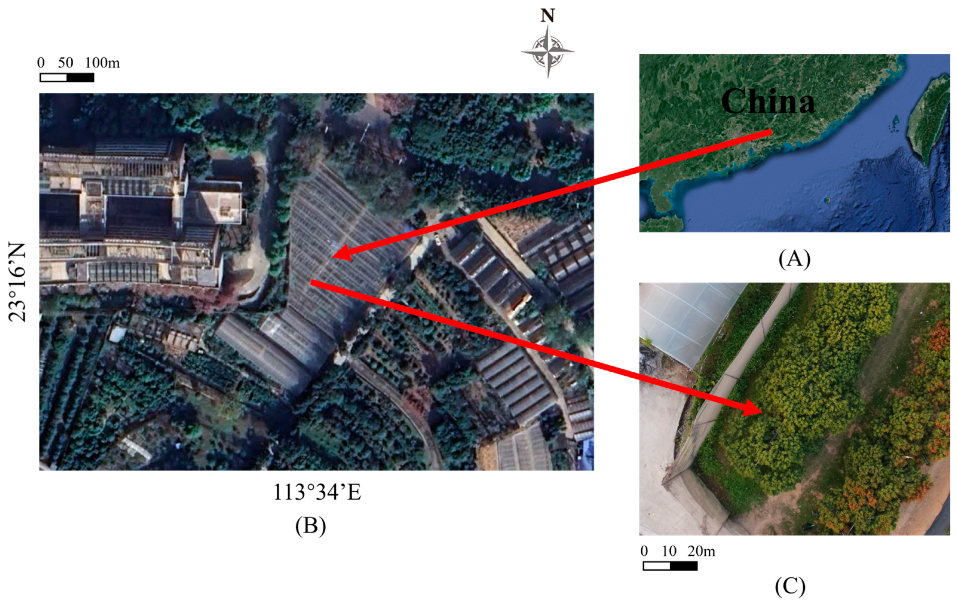
Figure 1. Study area. (A) Geographic location of Guangzhou within China; (B) location of Changgangshan Litchi Variety Garden in South China Agricultural University in Guangzhou; (C) top view of the study area taken from DJI Phantom 4 UAV.
Remotesensing 15 05767 g001
Figure 2. Data acquisition system.
Remotesensing 15 05767 g002
Figure 3. Comparison of dataset before and after screening outliers. (a) Gradient distribution of data before filtering. (b) Gradient distribution of data after filtering.
Remotesensing 15 05767 g003
Figure 4. Structure of the stacking algorithm.
Remotesensing 15 05767 g004
Figure 5. Experimental study flow chart.
Remotesensing 15 05767 g005
Figure 6. Statistical analysis of raw data.
Remotesensing 15 05767 g006
Figure 7. Correlation analysis during different periods. (a) Litchi fruit growth period; (b) litchi fruit growth period + autumn shoot period.
Remotesensing 15 05767 g007
Figure 8. Selection of independent variable combinations by full subset screening method when vegetation indexes were used as independent variables in the growth period of litchi.
Remotesensing 15 05767 g008
Figure 9. Results of different estimation models based on vegetation index + texture feature during the litchi fruit growth period. (a) SVR training set; (b) SVR validation set; (c) RF training set; (d) RF validation set; (e) KNR training set; (f) KNR validation set; (g) RR training set; (h) RR validation set; (i) stacking training set; (j) stacking validation set.
Remotesensing 15 05767 g009aRemotesensing 15 05767 g009b
Figure 10. Results of different prediction models based on vegetation index and texture feature during the litchi fruit growth period + autumn shoot period. (a) SVR training set; (b) SVR validation set; (c) RF training set; (d) RF validation set; (e) KNR training set; (f) KNR validation set; (g) RR training set; (h) RR validation set; (i) stacking training set; (j) stacking validation set.
Remotesensing 15 05767 g010aRemotesensing 15 05767 g010b
Table 1. Parameters of the multi-spectral camera.
Band NumberBand NameCentral Wave Length/nmWave Width/nmAsh Plate Reflectance/%
1Blue 4501625.095
2Green 5601626.648
3Red 6501626.687
4Red edge 7301626.680
5Near infrared8402628.000
Table 2. Optimal combination of arguments.
PeriodArgument TypeNumber of
Arguments
Optimal Combination of Arguments
Fruit growth periodVegetation index9CIred.edge, DVI, MCARI, MSAVI, OSAVI, RDVI, RVI2, SIPI, MTCI
Texture feature8Contrast (450 nm), Mean (540 nm), Mean (650 nm), Variancel (650 nm), Entropy (650 nm), Moment (650 nm), Homogeneity (730 nm), Contrast (840 nm)
Vegetation index + texture feature17CIred.edge, DVI, MCARI, MSAVI, OSAVI, RDVI, RVI2, SIPI, MTCI, Contrast (450 nm), Mean (540 nm), Mean (650 nm), Variancel (650 nm), Entropy (650 nm), Moment (650 nm), Homogeneity (730 nm), Contrast (840 nm)
Fruit growth period + autumn shoot periodVegetation index9CIred.edge, DVI, MCARI, NLI, OSAVI, RDVI, SIPI, TCARI, MTCI
Texture feature8Mean (450 nm), Dissimilarity (450 nm), Contrast (540 nm), Mean (650 nm), Contrast (650 nm), Dissimilarity (650 nm), Mean (840 nm), Second Moment (840 nm)
Vegetation index + texture feature17CIred.edge, DVI, MCARI, NLI, OSAVI, RDVI, SIPI, TCARI, MTCI, Mean (450 nm), Dissimilarity (450 nm), Contrast (540 nm), Mean (650 nm), Contrast (650 nm), Dissimilarity (650 nm), Mean (840 nm), Second Moment (840 nm)
Table 3. Validation results of different prediction models during the litchi fruit growth period.
PeriodArgumentModelTraining SetValidation Set
R2RMSERPDR2RMSERPD
Fruit growth periodVegetation indexesSVR0.872.72.00.823.81.7
RF0.932.22.80.883.32.1
KNR0.883.12.10.862.91.9
RR0.674.41.30.645.31.3
Stacking0.971.44.10.912.82.4
Texture featuresSVR0.813.01.70.654.71.3
RF0.933.22.80.634.51.3
KNR0.445.01.10.366.301.1
RR0.545.21.20.545.11.2
Stacking0.961.63.50.694.61.4
Vegetation indexes + texture featuresSVR0.952.03.10.833.41.8
RF0.971.54.20.922.52.6
KNR0.754.01.50.754.11.5
RR0.783.81.60.713.91.4
Stacking0.981.34.70.942.43.0
Table 4. Validation results of different estimation models during the litchi fruit growth period + autumn shoot period.
PeriodArgumentModelTraining SetValidation Set
R2RMSERPDR2RMSERPD
Fruit growth period + autumn shoot periodVegetation indexesSVR0.774.41.60.704.91.39
RF0.932.92.60.734.41.5
KNR0.665.11.30.595.31.2
RR0.615.41.30.595.41.2
Stacking0.971.44.10.912.82.4
Texture featuresSVR0.505.81.20.386.91.1
RF0.706.11.40.397.11.1
KNR0.306.91.10.296.91.0
RR0.396.41.10.376.71.1
Bagging0.555.71.20.426.71.1
Vegetation indexes + texture featuresSVR0.754.31.50.665.01.3
RF0.932.72.80.813.91.7
KNR0.694.91.40.675.01.4
RR0.684.61.40.645.41.3
Stacking0.952.13.20.843.91.9
Disclaimer/Publisher’s Note: The statements, opinions and data contained in all publications are solely those of the individual author(s) and contributor(s) and not of MDPI and/or the editor(s). MDPI and/or the editor(s) disclaim responsibility for any injury to people or property resulting from any ideas, methods, instructions or products referred to in the content.