Spatiotemporal Heterogeneity of Forest Fire Occurrence Based on Remote Sensing Data: An Analysis in Anhui, China

Abstract

A forest fire is a destructive disaster that is difficult to handle and rescue and can pose a significant threat to ecosystems, society, and humans. Since driving factors and their effects on forest fires change over time and space, exploring the spatiotemporal patterns of forest fire occurrence should be addressed. To better understand the patterns of forest fire occurrence and provide valuable insights for policy making, we employed the Geographically and Temporally Weighted Regression (GTWR) model to investigate the varying spatiotemporal correlations between driving factors (vegetation, topography, meteorology, social economy) and forest fires in Anhui province from 2012 to 2020. Then we identified the dominant factors and conducted the spatiotemporal distribution analysis. Moreover, we innovatively introduced nighttime light as a socioeconomic driving factor of forest fires since it can directly reflect more comprehensive information about the social economy than other socioeconomic factors commonly used in previous studies. This study applied remote sensing data since the historical statistic data were not detailed. Here, we obtained the following results. (1) There was a spatial autocorrelation of forest fires in Anhui from 2012 to 2020, with high-high aggregation of forest fires in eastern cities. (2) The GTWR model outperformed the Ordinary Least Squares (OLS) regression model and the Geographically Weighted Regression model (GWR), implying the necessity of considering temporal heterogeneity in addition to spatial heterogeneity. (3) The relationships between driving factors and forest fires were spatially and temporally heterogeneous. (4) The forest fire occurrence was mainly dominated by socioeconomic factors, while the dominant role of vegetation, topography, and meteorology was relatively limited. It’s worth noting that nighttime light played the most extensive dominant role in forest fires of Anhui among all the driving factors in the years except 2015.

1. Introduction

A forest fire is a kind of disaster with strong suddenness, great destructiveness, and difficulty in disposal and rescue. Forest fires significantly threaten ecosystems, communities, and humans, as strongly evidenced by extreme forest fires in the United States, Liangshan of China, and Australia. As we all know, meteorology, topography, vegetation, and human activities can affect forest ecosystems, potentially leading to more catastrophic forest fires. These driving factors’ temporal and spatial dynamic changes will profoundly affect forest fires’ temporal and spatial patterns. In this context, accurately identifying key driving factors and exploring the spatiotemporal patterns of forest fire occurrence is critical for protecting forest ecosystems and ensuring the safety of human life and property [1,2]. However, acquiring forest fire data and driving factors is a significant difficulty when studying forest fire occurrence’s spatial and temporal patterns. On the one hand, the historical records of forest fires from relevant departments are generally not detailed, and the fire data is coarse in spatial and temporal dimensions. On the other hand, forest fires involve many driving factors, and it is difficult to obtain complete field survey data or statistical data when the spatial study area is extensive and the temporal study period is prolonged. In this case, remote sensing data can be applied to investigate the spatiotemporal pattern of forest fire occurrence. There have been many studies on forest fires that have made extensive use of remote sensing data. For example, a large number of previous studies used fire remote sensing data from MODIS [3,4,5,6,7]. In recent years, a part of studies have used remote sensing data of fires from VIIRS [8,9,10,11,12]. Compared to MODIS, fire data from VIIRS have shown significant improvements in spatial resolution, observation amplitude and data quality. These studies indicate that remote sensing data are independent and objective, with high spatial and temporal resolution, and are well suited for scientific applications in support of forest fire monitoring and management.

In the past decades, many researchers have conducted studies to identify the driving factors of forest fires [4,13,14,15,16,17,18,19,20]. Early studies mainly focused on exploring the impact of meteorological factors (e.g., rainfall, temperature) on forest fires. More recent studies have begun to realize the impact of vegetation, topography, human activity, and other socioeconomic factors and have carried out more comprehensive analyses [2,13,14,15,21,22,23,24,25,26]. These recent studies indicated that simultaneous consideration of potential factors in different aspects is necessary to identify the key driving factors. Gross domestic product (GDP) has often been used as a factor to characterize socioeconomic influences [16,27]. However, administrative divisions are generally used as the statistical unit of GDP data, which cannot be used for spatial studies requiring fine resolutions. When not considering spatial heterogeneity, GDP can represent socioeconomic development for studying the correlation between socioeconomic development and forest fires. When considering the spatial and temporal heterogeneity of forest fire occurrence, using the statistical GDP data will undoubtedly reduce the accuracy of the model results. Scholars in related fields have used nighttime light, settlement density, and land use data to estimate and produce GDP spatial grid data [28], but the GDP spatial grid data cannot meet the needs of this study in the temporal dimension. Compared with GDP, the intensity information of nighttime lights can more directly reflect the difference in human activities. Nighttime light covers information closely related to the city’s development, such as traffic roads and residential places, and can better reflect the comprehensive information of socioeconomic influences than GDP. More importantly, its remote sensing data has the advantages of high spatiotemporal resolutions and are easily accessible. Therefore, this study attempted to use nighttime light instead of GDP as a factor reflecting socioeconomic development affecting forest fires. Nighttime light has been widely used to explore the impact of human activities on urbanization, socioeconomic indicators, major emergencies, and public health [29,30,31]. However, it has yet to be extensively adopted to discuss the impact of human activities on forest fires.

Methodologically, many models devoted to studying the patterns of forest fire occurrence by revealing the relationships between forest fires and their driving factors have been developed, including logistic regression, classification tree, regression trees, random forests, ANNs, SVM, LightGBM [13,26,32,33,34]. These methods focus on a global perspective and assume that all variables are stationary and independent in spatial and temporal dimensions in the study area. However, driving factors such as topography, vegetation, meteorology, and social economy show high degrees of variation in a wide range of spatial or temporal dimensions. Some studies have shown that varied rather than stable relationships would be more reasonable when large geographical study areas are involved—e.g., [2,35]. Accordingly, ignoring local variations will undoubtedly reduce the model’s reliability and restrict the understanding of the spatiotemporal patterns of forest fire occurrence. The traditional global linear regression model, Ordinary Least Squares (OLS) regression, uses “global correlation” to measure the correlation between forest fire occurrence and its driving factors. It can only estimate “average” or “global” parameters and cannot reflect the spatiotemporal-varying properties of variables. The Geographically Weighted Regression (GWR) model, a local regression model that can describe the local spatial variation of the coefficients, has received increasing attention in the literature as a spatial analysis technique. Moreover, the GWR model has been applied to explore the spatial heterogeneity of the relationship between forest fire and its drivers in recent years [2,15]. In addition, some studies have divided the study area into different parts to investigate the spatial heterogeneity of forest fire occurrence [36]. However, the driving factors of forest fires vary over time. Therefore, the role of driving factors in explaining forest fire occurrence also changed over time; some decreased their explaining power, while others increased. Driving factors that were important at the beginning of the study period may be less critical at the end. However, how these driving factors changed over time has rarely been explored. Thus, this study proposed the Geographically and Temporally Weighted Regression (GTWR) model to capture the varying spatiotemporal relationships between driving factors. Based on the traditional GWR model, the GTWR model developed by Huang [20] incorporates the time effect, thereby providing a method for studying the relationships between forest fires and their driving factors, considering spatial and temporal non-stationarity simultaneously [37,38,39]. Additionally, the GTWR model has been proven to be a robust technique for capturing spatial and temporal heterogeneity [40]. It has been widely used in several fields, such as economy, transportation, and air pollution, but it has yet to be widely used for forest fires.

Understanding the spatiotemporal patterns of forest fire occurrence is essential for making efficient forest fire prevention and management strategies. Therefore, we employed the GTWR model to investigate the spatiotemporal relationships between forest fires and driving factors and applied this model to a large-scale spatial range (Anhui province, China). Moreover, this paper innovatively introduced nighttime light as a socioeconomic driving factor. In principle, this framework can be popularized and transferred to other regions. The main objectives of this study are (1) to explore the feasibility of the GTWR model in spatiotemporal modeling of forest fire occurrence, (2) to investigate the applicability of nighttime light as a socioeconomic factor influencing forest fire occurrence, and (3) to explore the spatiotemporal variations of the correlations between forest fires and driving factors to provide some valuable insights for forest fire policy.

2. Materials and Methods

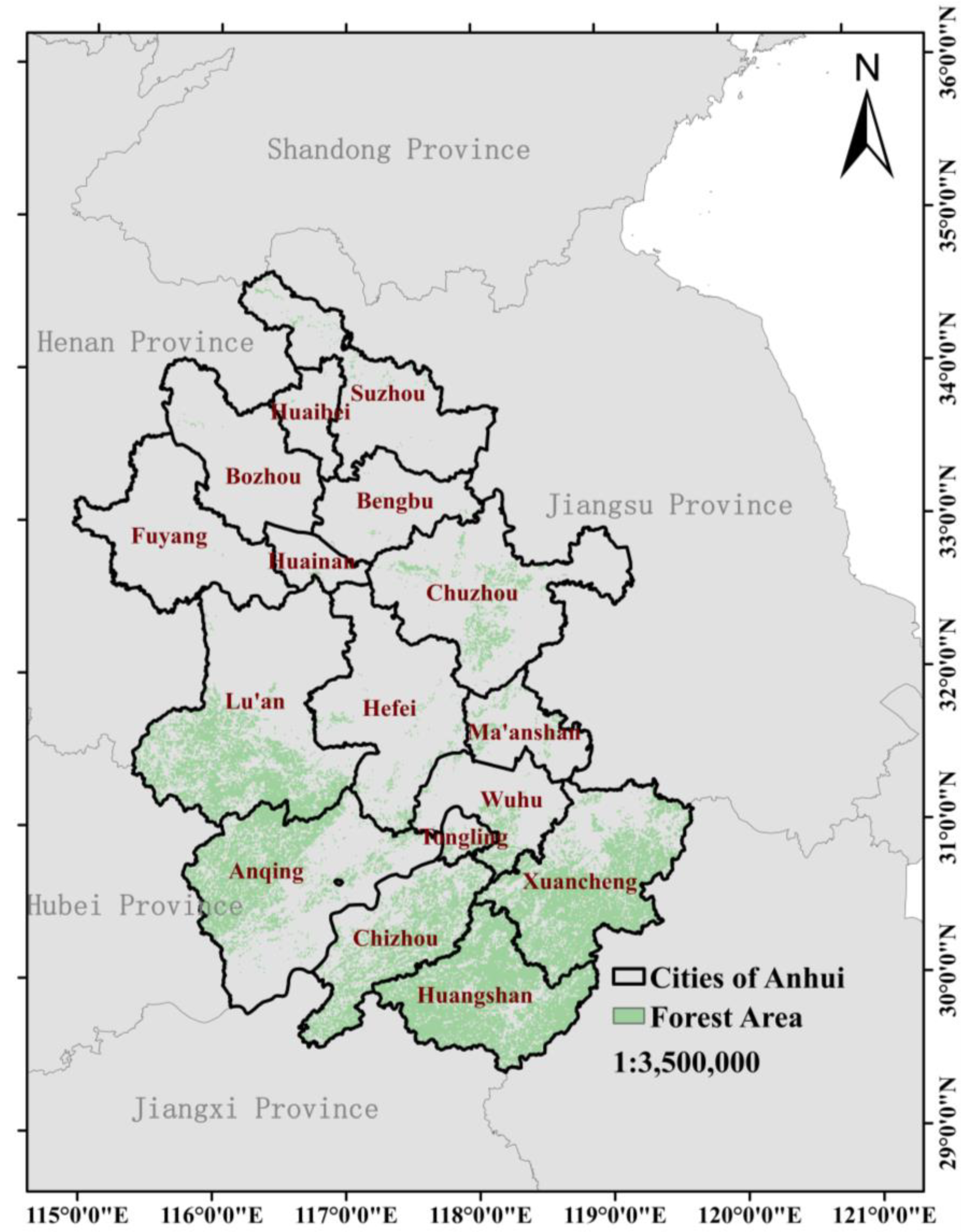
2.1. Study Area

Anhui province (Figure 1) is a critical province of forest area in south China. Anhui province has a mild climate with obvious monsoons and four distinct seasons. The province’s annual temperature is 14–16 °C, and the annual average precipitation is 800–1600 mm. It has sufficient sunshine with an average annual sunshine of 1800–2500 h. The topography is complex, intertwining with plains, hills, and mountains. Moreover, there are rich and diverse wild plant resources, and the forest vegetation has prominent transition characteristics from north to south. Such natural and geographical conditions provide the environmental basis for the occurrence of forest fires. Moreover, with the expansion of forest areas and the increase in human activities brought about by the construction of forest cities, forest fires have occurred frequently in Anhui province in recent years. According to Anhui province’s policy of continuous afforestation and accelerating the construction of forest cities in the coming years, we can grab a signal that Anhui is making significant efforts to expand the forest area and build forest cities, indicating that more and more human activities will be involved in the forest area. The ideal natural geographical conditions, the continuous expansion of forest area, and the increase of human activities will increase the risk of forest fires in Anhui province in the future. Therefore, it is imperative to identify the driving factors of forest fires and explore the spatial-temporal patterns of forest fire occurrence in Anhui province.

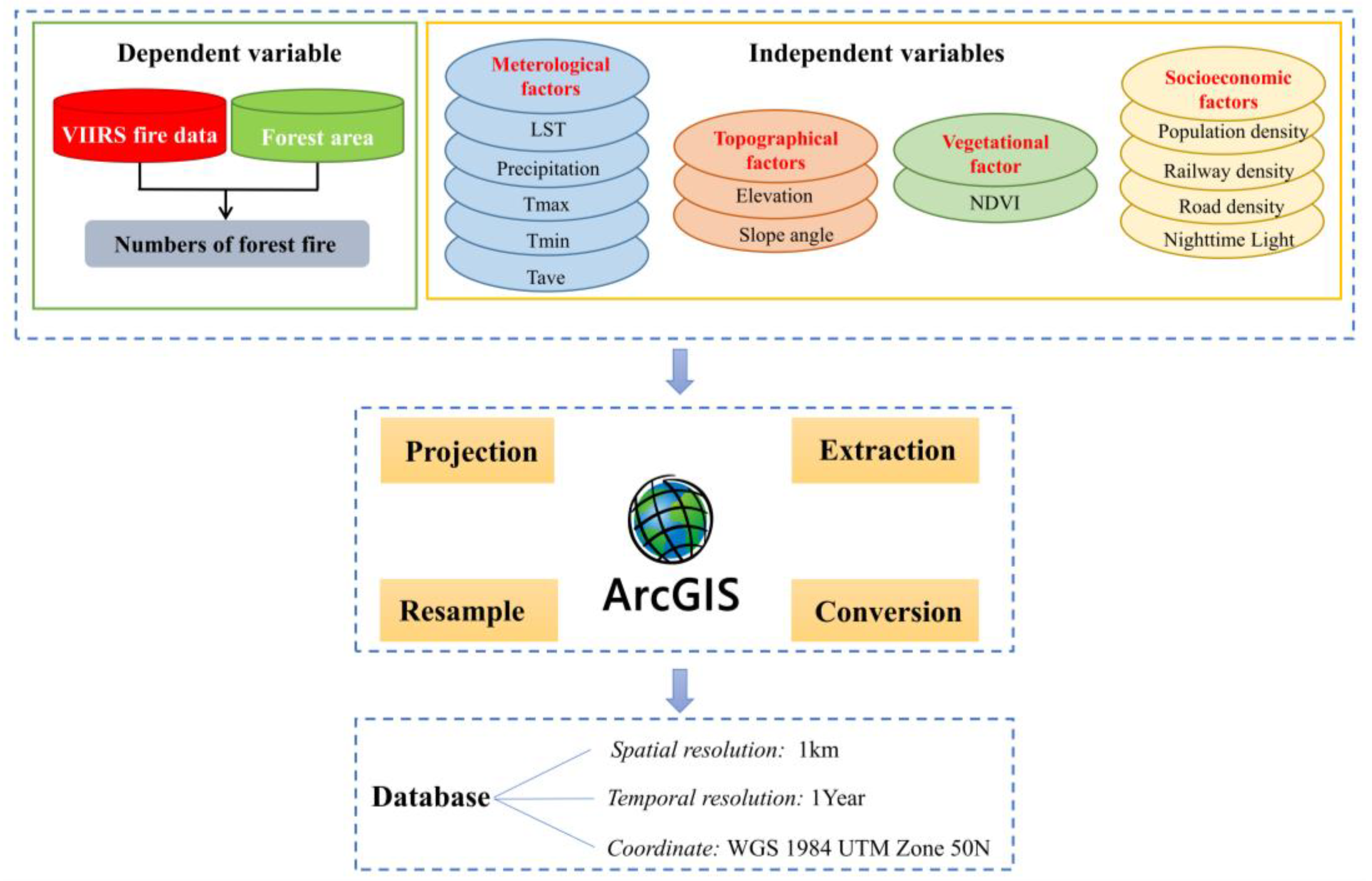
2.2. Variable Selection

This study selected the number of forest fires as the dependent variable. Previous studies often acquired fire data from the Moderate Resolution Imaging Spectroradiometer (MODIS) [4,17,26,32,41,42,43,44,45,46,47]. Compared with MODIS, Visible Infrared Imaging Radiometer Suite (VIIRS) fire data has significant improvement in spatial resolution, observation amplitude, and data quality. As a result, the VIIRS fire data is better suited to support fire management, near-real-time wildfire alert systems, and other scientific applications that require improving mapping fidelity. Therefore, we extract the forest fire data from 2012 to 2020 from VIIRS 375 m Active Fire Product with a spatial resolution of 375 m and a temporal resolution of one year.

Accurate and comprehensive identification of potential drivers is critical for forest fire research. The selection of these driving factors follows two basic principles. One is that the source of data is reliable and authorized; the other is that these factors are associated with the occurrence of forest fires. We selected 12 driving factors based on their potential influence on forest fire occurrence, extensive literature review, and high spatial and temporal resolution availability. As shown in

Table 1. Description and source of the data used in this study.

Category	Item	Abbreviation	Spatial Resolution	Source
Dependent variable	Forest fire frequency	FFF	375 m	VIIRS https://earthdata.nasa.gov/earth-observation-data, accessed on 1 September 2021
Topographical factors	Slope angle	SAG	90 m	Geospatial Data Cloud https://www.gscloud.cn/, accessed on 1 September 2021
	Elevation	ELE		Resource and Environment Science and Data Center https://www.resdc.cn/, accessed on 1 September 2021
Vegetational factor	Normalized Difference Vegetation Index	NDVI	1000 m	Resource and Environment Science and Data Center https://www.resdc.cn/, accessed on 1 September 2021
Meteorological factors	Annual average land surface temperature	LST	5600 m	Zenodo https://zenodo.org/, accessed on 1 September 2021 NASA Earth Data https://lpdaac.usgs.gov/products/mod11c3v006/, accessed on 1 September 2021
	Annual accumulated precipitation	PREP	1000 m	National Earth System Science Data Center http://www.geodata.cn/, accessed on 1 September 2021
	Annual average maximum temperature	Tmax		National Earth System Science Data Center http://www.geodata.cn/, accessed on 1 September 2021
	Annual average minimum temperature	Tmin		National Earth System Science Data Center http://www.geodata.cn/, accessed on 1 September 2021
	Annual average temperature	Tave		National Earth System Science Data Center http://www.geodata.cn/, accessed on 1 September 2021
Socioeconomic factors	Railway density	RAD	/	Geographic Information Professional Knowledge Service System http://kmap.ckcest.cn/, accessed on 1 September 2021 Open Street Map https://download.geofabrik.de/, accessed on 1 September 2021
	Road density	ROD	/	Geographic Information Professional Knowledge Service System http://kmap.ckcest.cn/, accessed on 1 September 2021 Open Street Map https://download.geofabrik.de/, accessed on 1 September 2021
	Population density	POP	1000 m	WorldPOP https://hub.worldpop.org/project/categories?id=3, accessed on 1 September 2021
	Nighttime light	NTL	500 m	Earth Observation Group https://payneinstitute.mines.edu/eog/, accessed on 1 September 2021

, we divided these factors into four categories: topographical, vegetational, meteorological, and socioeconomic factors, and collected data from authorized websites [48,49,50,51].

Topographical factors. In this work, topographical factors contain elevation and slope angle. The temperature, moisture, and wind are associated with elevation, influencing vegetation structure, fuel moisture, and air humidity [24]. Slope angle is typically highly correlated with the formation and evolution of forest fires [19]. Steep topography is essential in forming local winds, accelerating the spread of fires [4]. Additionally, slope angle may affect ignitions by limiting accessibility, with a threshold of 20° being mentioned as a restrictive factor for harvesting in forest conservation studies [13,18].

Vegetation factor. The vegetation factor is the Normalized Difference Vegetation Index (NDVI), which describes vegetation density. NDVI characterizes the vegetation coverage near the surface, which directly determines the likelihood of a forest fire [19,20].

Meteorological factors. It has become a broad consensus that meteorological factors (e.g., temperature and precipitation) affect forest fires by affecting fuel accumulation and moisture. Based on previous studies and data availability of the study period [13,14,15,20,27], this work selects annual maximum temperature, annual minimum temperature, annual average temperature, annual accumulated precipitation, and annual average land surface temperature as the meteorological factors.

Socioeconomic factors. The fact that human activities are closely related to forest fires has been clarified in previous studies [14,15,17,27,52,53,54]. These studies identified the presence of roads and railways as essential factors in human-caused forest fires. Human influence, such as changes in vegetation conditions due to the construction of roads or railways, and fire sources generated by mobile vehicles on the roads, will further increase the probability of forest fire [20,55]. In the past, some researchers used Gross Domestic Product (GDP) and population density to reflect human activities [12,13,16,24,25]. Nevertheless, the GDP generally suffers from coarse spatial resolutions. Therefore, this study employs nighttime light to replace the GDP to meet the precision requirements of this study. Nighttime light data are remote sensing images with high spatiotemporal resolutions and based on artificial light of human activities. Thus, the light intensity information can more directly and precisely reflect the differences in human activities than GDP. To summarize, nighttime light, population density, road density, and railway density are the socioeconomic factors to characterize human activities.

2.3. Data Processing

The data process was completed on the ArcGIS 10.5 platform. Considering the inconsistent spatiotemporal resolutions of independent variables with different data sources, we resampled all the independent variables to grids with a spatial resolution of 1 km and a temporal resolution of 1 year. The dependent variable of each grid was obtained by summing the number of forest fires within a 1 km × 1 km grid. Finally, there were 5198 matched observation points (each grid cell corresponds to one observation point) incorporating dependent and independent variables from 2012 to 2020. The data processing workflow is illustrated in Figure 2. Before implementing the GTWR model, we used the variance inflation factor (VIF) to test collinearity among independent variables on the R Studio platform. The independent variables with VIF values of more than ten will be eliminated. Since the magnitudes of raw data varied greatly among independent variables, putting the raw data into the GTWR model will amplify the role of variables with larger magnitudes and weaken the role of variables with smaller magnitudes. Hence, this study used the Z-score method to standardize the independent variable data.

2.4. Spatial Autocorrelation Analysis

Spatial autocorrelation is a kind of spatial data analysis method of studying whether observations at different locations in space are correlated and how correlated they are. The spatial autocorrelation in the dependent variable is a pre-condition for the application of the GTWR model [40]. Thus, this study employed Global spatial autocorrelation analysis and Local spatial autocorrelation analysis to evaluate the spatial autocorrelation of forest fires in Anhui province.

2.4.1. Global Spatial Autocorrelation Analysis

To investigate the spatial autocorrelation of forest fires, we executed Global spatial autocorrelation analysis on ArcGIS 10.5 platform. The most commonly used global spatial autocorrelation analysis technique is $Global Mora{n}^{\prime }s I$, it can be expressed as [56]:

$$Global Mora{n}^{\prime }s I=\frac{n}{{{\displaystyle \sum }}_{i=1}^n{{\displaystyle \sum }}_{j=1}^n{w}_{ij}}\frac{{{\displaystyle \sum }}_{i=1}^n{{\displaystyle \sum }}_{j=1}^n{w}_{ij}\left(y_i-\overline{y}\right)\left(y_j-\overline{y}\right)}{{{\displaystyle \sum }}_{i=1}^n{\left(y_i-\overline{y}\right)}^2}$$

(1)

where $n$ represents the number of cities in Anhui province; $w_{ij }$ is the weight between city $i$ and $j$; $y_i$ and $y_j$ represents the number of forest fires in city $i$ and $j$, respectively; and $\overline{y}$ is the average number of forest fires in all cities. The value of $Global Mora{n}^{\prime }s I$ range from [−1, 1]. $Global Mora{n}^{\prime }s I$ is close to 0 means that the distribution of forest fire frequency is random. If $Global Mora{n}^{\prime }s I$ is close to −1, the distribution of forest fire frequency is dispersed in space. If $Global Mora{n}^{\prime }s I$ is close to 1, forest fire frequency is clustered in space, that is, there exists spatial autocorrelation in forest fires.

To judge spatial autocorrelation, it is necessary to test the significance of $Global Mora{n}^{\prime }s I$, and the significance level in this study is set as $p<0.05$. The null hypothesis of $Global Mora{n}^{\prime }s I$ is that the forest fire frequency is spatial independent, indicating that $Global Mora{n}^{\prime }s I$ is close to 0. Here, we applied Z-score method for the significance test. It was calculated as the following:

$$Z\left(I\right)=\frac{I-E\left(I\right)}{\sqrt{Var\left(I\right)}}$$

(2)

$$E\left(I\right)=-\frac{1}{n-1}$$

(3)

$$Var\left(I\right)=E\left[I^2\right]-E{\left[I\right]}^2$$

(4)

$E \left(I\right)$ and $Var \left(I\right)$ are the expectation and the standard deviation of the, respectively. The significance level in this study is set as $p<0.05$.

2.4.2. Local Spatial Autocorrelation Analysis

Global spatial autocorrelation analysis can reveal the degree of spatial dependence in the distribution of forest fires from the perspective of the whole Anhui province but cannot identify local differences in the distribution of forest fires. Therefore, we employed $Local Mora{n}^{\prime }s I$ to derive the local spatial correlation of forest fire frequency among different cities on the ArcGIS 10.5 platform, which can be expressed as follows:

$$Local Mora{n}^{\prime }s I=\frac{n\left(y_i-\overline{y}\right){{\displaystyle \sum }}_{j=1}^n{w}_{ij}(y_j-\overline{y})}{{{\displaystyle \sum }}_{i=1}^n{\left(y_i-\overline{y}\right)}^2}$$

(5)

where $n$ represents the number of cities in Anhui province; $w_{ij}$ represents the weight of the spatial relationship between city $i$ and $j$; $y_i$ represents the forest fire frequency of city $i$; and $\overline{y}$ is the average number of forest fires in all cities in Anhui.

Then, we can obtain the Local Indicators of Spatial Association (LISA) map based on $Local Mora{n}^{\prime }s I$. The local spatial correlation mode of LISA map can be divided into several types of correlations: high-high cluster, low-low cluster, high-low outlier, low-high outlier, and not significant. $Local Mora{n}^{\prime }s I>0$ indicates the spatial positive correlation between the forest fire frequency of adjacent cities, which is represented as high-high cluster or low-low cluster. $Local Mora{n}^{\prime }s I<0$ indicates the spatial negative correlation between the forest fire frequency of adjacent cities, which is expressed as high-low outlier or low-high outlier. $Local Mora{n}^{\prime }s I=0$ indicates there is no significant correlation between the forest fire frequency of different cities.

2.5. GTWR Model

According to the work of [37,38], the general structure of the GTWR model developed in this study is described as follows:

$$y_i={\beta }_0\left(u_i,v_i,t_i\right)+{\displaystyle \sum }_{k=1}^d{\beta }_k\left(u_i,v_i,t_i\right)x_{ik}+{\epsilon }_i$$

(6)

where $i \left(i=1,2, \dots , n\right)$ denotes the observation points; $y_i$ refers to dependent variable, $x_{ik}$ represents the $k$th independent variable at point $i$. $\left(u_i,v_i,t_i\right)$ is the coordinates of the observation point $i$, and $u_i,v_i,t_i$ is the $X$ coordinate, $Y$ coordinate, and time coordinate, respectively; ${\beta }_0\left(u_i,v_i,t_i\right)$ is the intercept value; and ${\beta }_k\left(u_i,v_i,t_i\right)$ denotes a set of coefficients at point $i$; ${\epsilon }_i$ is the random error.

The coefficients ${\beta }_0\left(u_0,v_0,t_0\right),{\beta }_1\left(u_0,v_0,t_0\right),\dots ,{\beta }_d\left(u_0,v_0,t_0\right)$ at any regression point $\left(u_0,v_0,t_0\right)$ in the space-time domain can be estimated by using the observation value $\left(y_i,x_{i1},x_{i2},\dots ,x_{ik}\right),i=1,2,\dots ,n$ at the observation point $\left(u_i,v_i,t_i\right)$. However, the importance (weight) of different observation points for estimating the coefficients at the regression point $\left(u_0,v_0,t_0\right)$ is not the same. According to the well-known First Law of Geography: everything is related to everything else, but near things are more related than distant things. Thus, the closer the observation point $\left(u_i,v_i,t_i\right)$ is to regression point $\left(u_0,v_0,t_0\right)$, the bigger weight was assigned in estimating the coefficients at point $\left(u_0,v_0,t_0\right)$. Based on a local weighted least squares algorithm:

$${\displaystyle \sum }_{i=1}^n{\left[y_i-{\beta }_0\left(u_0,v_0,t_0\right)-{\displaystyle \sum }_{k=1}^d{\beta }_k\left(u_0,v_0,t_0\right)x_{ik}\right]}^2{w}_i\left(u_0,v_0,t_0\right)$$

(7)

By taking the partial derivative of Equation (7) with respect to ${\beta }_0\left(u_0,v_0,t_0\right)$ and ${\beta }_k\left(u_0,v_0,t_0\right)$, we can attain the estimated coefficients expressed in the form of matrix as follows:

$$\widehat{\beta }\left(u_0,v_0,t_0\right)={\left[X^{T}W\left(u_0,v_0,t_0\right)X\right]}^{-1}{X}^{T}W\left(u_0,v_0,t_0\right)Y$$

(8)

In Equation (7), $w_i\left(u_0,v_0,t_0\right)$ is the weight assigned to observation point $\left(u_i,v_i,t_i\right)$. In Equation (8), $X$ is the matrix of independent variables, $Y$ is the matrix of dependent variables, the spatiotemporal weighted matrix $W\left(u_0,v_0,t_0\right)$ is an $n\times n$ diagonal matrix that can be described as follows:

$$\begin{array}{c}W\left(u_0,v_0,t_0\right)\\ =diag\left(w_1\left(u_0,v_0,t_0\right),w_2\left(u_0,v_0,t_0\right),\dots w_i\left(u_0,v_0,t_0\right)\dots w_n\left(u_0,v_0,t_0\right)\right)\end{array}$$

(9)

In this study, we eliminated Tave and LST by VIF > 10 in the collinearity test. Therefore, the final variables involved in model construction include SAG, ELE, NDVI, PREP, Tmax, Tmin, RAD, ROD, NTL, and POP. The GTWR model of the relationship between the number of forest fires (NFF) and its driving factors can be expressed as follows:

$$\begin{array}{c}NF{F}_i={\beta }_0\left(u_i,v_i,t_i\right)+{\beta }_1\left(u_i,v_i,t_i\right)\times SAG+{\beta }_2\left(u_i,v_i,t_i\right)\times ELE\\ \hspace{1em}\hspace{1em}\hspace{1em}\hspace{1em}\hspace{1em}\hspace{1em}\hspace{1em}+{\beta }_3\left(u_i,v_i,t_i\right)\times NDVI+{\beta }_4\left(u_i,v_i,t_i\right)\times PREP\\ \hspace{1em}\hspace{1em}\hspace{1em}\hspace{1em}\hspace{1em}\hspace{1em}\hspace{1em}+{\beta }_5\left(u_i,v_i,t_i\right)\times T_{min}+{\beta }_6\left(u_i,v_i,t_i\right)\times T_{max}\\ \hspace{1em}\hspace{1em}\hspace{1em}\hspace{1em}\hspace{1em}\hspace{1em}\hspace{1em}+{\beta }_7\left(u_i,v_i,t_i\right)\times RAD+{\beta }_8\left(u_i,v_i,t_i\right)\times ROD\\ \hspace{1em}\hspace{1em}\hspace{1em}\hspace{1em}\hspace{1em}\hspace{1em}\hspace{1em}+{\beta }_9\left(u_i,v_i,t_i\right)\times NTL+{\beta }_{10}\left(u_i,v_i,t_i\right)\times POP+{\epsilon }_i\end{array}$$

(10)

where $\left(u_i,v_i,t_i\right)$ are the central coordinates of a grid cell and $i$ is the central point of that grid cell. $u_i$, $v_i$ is the $X$ coordinate and the $Y$ coordinate in meters, and $t_{i }$ is the time coordinated in years. $NF{F}_i$ is the number of forest fires in the grid cell where point $i$ is located on time $t_i$. SAG, ELE, NDVI, PREP, Tmax, Tmin, RAD, ROD, NTL, and POP represent the value of slope angle, elevation, Normalized Difference Vegetation Index, annual accumulated precipitation, annual minimum temperature, annual maximum temperature, railway density, road density, nighttime light, and population density respectively at point $i$ on time $t_i$.

The identification of weight $w_i\left(u_0,v_0,t_0\right)$ in (9) is one critical step in model construction. In this study, $w_i\left(u_0,v_0,t_0\right)$ is a spatiotemporal weight based on the Gaussian distance decay-based function in space-time domains, which is described as follows:

$$w_i\left(u_0,v_0,t_0\right)=\exp \left[-\frac{{\left(d_{i0}^{ST}\right)}^2}{h^2}\right]$$

(11)

where $h$ is a positive parameter named spatiotemporal bandwidth, and $d_{i0}^{ST}$ is the spatial-temporal distance between points $\left(u_i,v_i,t_i\right)$ and point $\mathrm{s} \left(u_0,v_0,t_0\right),$ which can be calculated based on the Euclidean distance formula:

$$d_{i0}^{ST}=\sqrt{\lambda \left[{\left(u_i-u_0\right)}^2-{\left(v_i-v_0\right)}^2\right]+{\left(t_i-t_0\right)}^2}$$

(12)

where $\lambda$ is the non-negative scale factor. However, location and time are usually measured in different units (in our case, location in meters and time in years); thus, they have different scale effects. It seems to be more appropriate to add $\lambda$ to balance the effects of spatial and temporal distances when combining the spatial and temporal items. Therefore, $w_i\left(u_0,v_0,t_0\right)$ can be expressed as follows:

$$w_i\left(u_0,v_0,t_0\right)=exp\left\{-\left[\frac{\lambda \left[{\left(u_i-u_0\right)}^2-{\left(v_i-v_0\right)}^2\right]+{\left(t_i-t_0\right)}^2}{h^2}\right]\right\}$$

(13)

The selection of bandwidth $h$ is another important step in model calculation. A cross-validation (CV) method is commonly used to select this parameter. Assume that ${\widehat{y}}_i\left(h\right)$ is the predicted value from the GTWR model with bandwidth $h$. Then, the sum of the squared error can be written as follows:

$$CV\left(h,\lambda \right)={\displaystyle \sum }_{i=1}^n{\left(y_i-{\widehat{y}}_i\left(h,\lambda \right)\right)}^2$$

(14)

The optimal bandwidth can be derived automatically with an optimization technique by minimizing (14) according to the corrected Akaike information criterion (AIC) [37].

3. Results

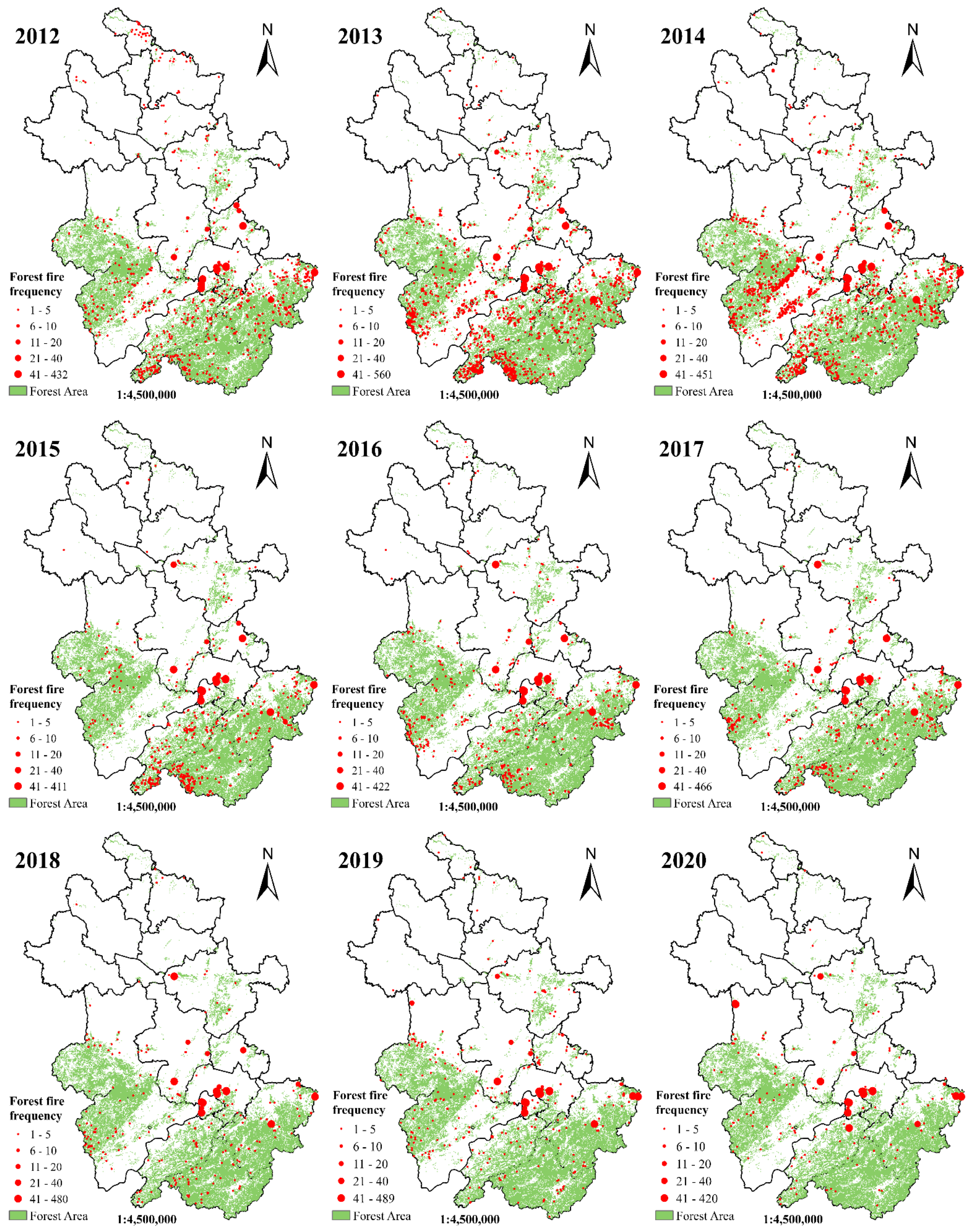
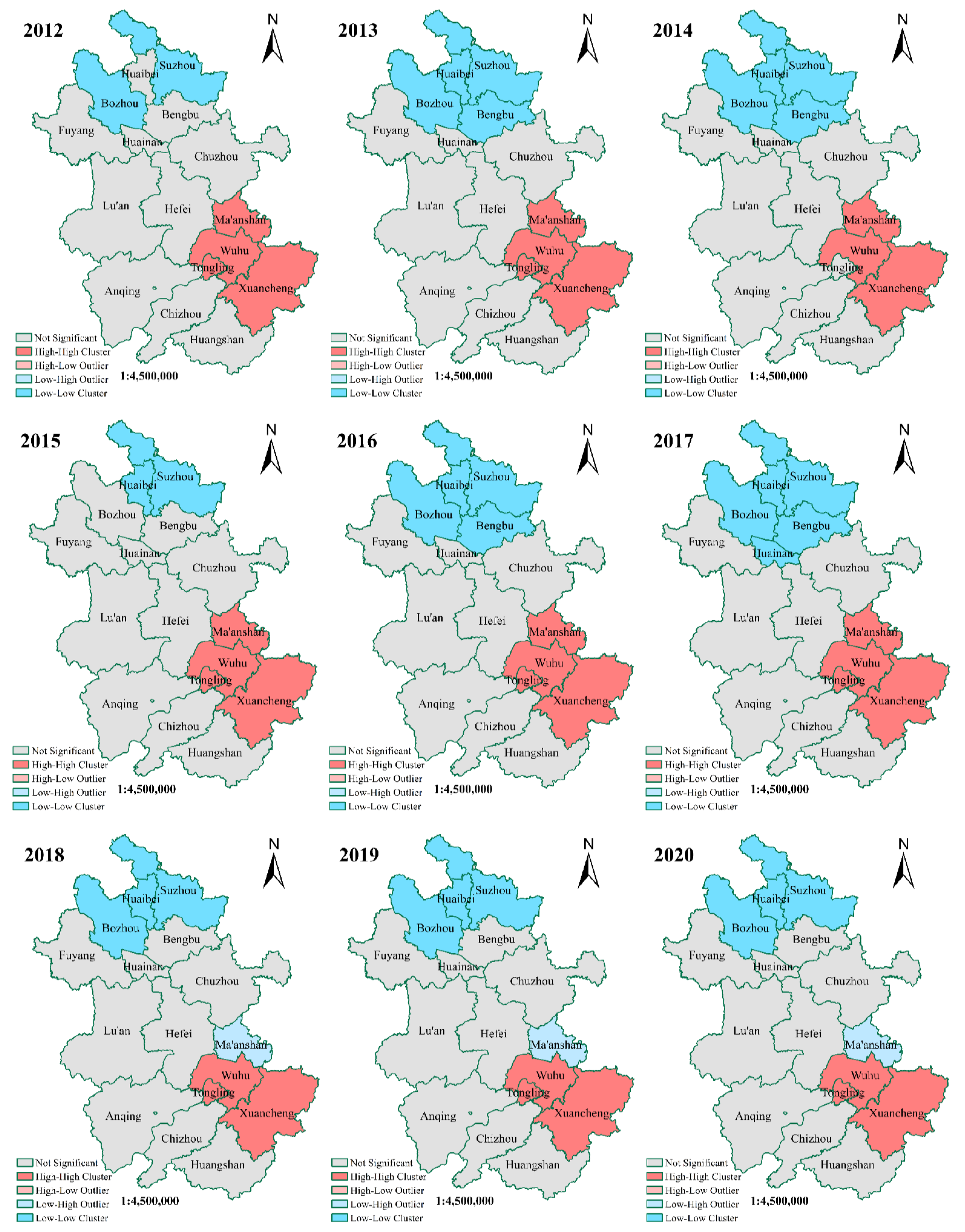
3.1. Spatial Autocorrelation of Forest Fires

Figure 3 intuitively displays the spatial distribution of annual forest fire points and their frequency in the Anhui province. The red dots in Figure 3 represent the location of the forest fire points, and bigger red dots mean more forest fires occurred. In Figure 3, relatively high-frequency forest fires were mainly concentrated in Wuhu, Xuancheng, Tongling, Ma’anshan, and Hefei. We observed dense forest fire points in Lu’an, Anqing, Chizhou, Huangshan, and Xuancheng from 2012 to 2014. From 2015 to 2020, the number of forest fire points in Anhui province decreased significantly, and the distribution of forest fire points became more and more dispersed.

Table 2. The results of global spatial autocorrelation test.

Year	2012	2013	2014	2015	2016	2017	2018	2019	2020
Moran’s I	0.81	0.74	0.36	0.66	0.65	0.66	0.47	0.51	0.45
Z-score	4.17	3.75	1.98	3.76	3.75	3.77	2.88	2.99	2.73
p-value	0.00003	0.00018	0.04760	0.00017	0.00017	0.00016	0.00400	0.00281	0.00628

and Figure 4 show the results of global and local spatial autocorrelation tests, respectively. The values of $\mathrm{Global} \mathrm{Mora} \mathrm{n} \prime \mathrm{s} \mathrm{I}$ were all positive, and Z-scores were all larger than 1.96, which confirms the presence of a significant (p < 0.05) spatial clustered pattern in annual forest fires of Anhui from 2012 to 2020. In Figure 4, we observed high-high clustering mainly in eastern cities, such as Ma’anshan, Wuhu, Tongling, and Xuancheng. Low-Low clustering was mainly distributed in northern cities, such as Bozhou, Suzhou, Huaibei, and Bengbu, which were the cities with less forest area and forest fire points in Figure 3. The above findings suggested that forest fire prevention and management in some of the eastern cities should be emphasized, such as Wuhu, Tongling, and Xuancheng, which were high-high forest fire clustering cities almost every year over the study period.

3.2. Performance of GTWR Model

In

Table 3. Model comparison results.

Indicator	Model
	OLS	GWR	GTWR
AIC	30,834.97	28,597.52	23,985.66
Adjusted R2	0.13	0.67	0.84

, we compared the performance and goodness of fit of the OLS, GWR, and GTWR models using the indicator of Akaike Information Criterion (AIC) and Adjusted R2. The results showed that the GTWR model performed the best and the OLS model performed the worst, indicating that it is necessary to consider spatial and temporal heterogeneity when studying forest fire occurrence patterns. To evaluate the GTWR model’s performance, we executed a five-fold Cross Validation (CV) approach to validate the robustness of the model. For CV, we randomly split the dataset into five subsets, then treated one of the subsets as the testing data and fitted the model with the remaining four subsets. Finally, we repeated the above process five times to ensure that all data were tested. Meanwhile, we used the Adjusted R2, the root-mean-square error (RMSE), and the mean absolute error (MAE) to evaluate the performance of the GTWR model quantitatively. The results are listed in

Table 4. Performance of the GTWR model in cross-validation.

Fold	Model Fitting			Model Validation
	Adjusted R2	RMSE	MAE	Adjusted R2	RMSE	MAE
1	0.75	2.57	0.96	0.65	3.05	1.16
2	0.69	2.76	1.04	0.68	3.00	1.15
3	0.80	2.12	0.89	0.60	3.90	1.35
4	0.76	2.50	0.93	0.69	2.86	1.07
5	0.89	1.76	0.72	0.72	2.11	0.88

.

3.3. Varying Spatiotemporal Relationships between Forest Fires and Driving Factors

An important feature of the GTWR model is that the estimated coefficients can be visualized and analyzed to reveal the spatiotemporal heterogeneity of forest fire occurrence by observing the spatial and temporal variation of the correlation coefficients between driving factors and forest fires. We performed Kriging interpolation for the estimated coefficients of driving factors on ArcGIS 10.5 to understand the spatial patterns of forest fires better. In the temporal analysis, this study analyzed the occurrence of forest fires in Anhui province from the temporal dimension at both provincial and municipal levels. At the provincial level, we focused on the breadth of the positive influence of driving factors on forest fire occurrence varying over time. At the municipal level, we focused on the degree of influence of driving factors on forest fire occurrence varying over time. The temporal analyses at both levels combined the driving factors’ temporal changes to reveal the temporal heterogeneity of forest fire occurrence. In the provincial-level analysis, we used the spatial proportion of positive correlation coefficients between driving factors and forest fires (hereafter referred to as “positive coefficients”) to describe the breadth of driving factors on forest fire occurrence. Since the data used in the GTWR model in this study were standardized, the coefficients obtained from the GTWR model can reflect the degree of the driving factors on forest fires, i.e., their relative importance on forest fire occurrence. However, these coefficients varied spatially on a grid basis, leading to difficulties visualizing them in the time dimension. To facilitate the time-dimensional analysis, we chose a compromise solution of averaging the driving factor coefficients at the municipal level. Therefore, in the analysis at the municipal level, we used the average correlation coefficients between the driving factors and forest fires to indicate the degree of influence of the driving factors on forest fire occurrence. To facilitate the observation of temporal trends, this study connects the points in the figure with dashed lines. For the spatial analysis, this study used ArcGIS 10.5 to plot the spatial distribution of the correlation coefficients between driving factors and forest fires for each year of the study period (Figures S1–S10). We manually set zero as the threshold in the legend to distinguish positive and negative effects. Based on the range of coefficient values, we artificially divided the coefficients into three negative and three positive classes, representing different degrees of correlation: slight, distinct, and extreme. A larger positive coefficient represents a more significant positive correlation, and a smaller negative coefficient represents a more significant negative correlation.

Vegetational factors. There were spatial and temporal differences in the influence of NDVI on forest fire occurrence. At the provincial level (Figure 5), the mean NDVI in the Anhui province fluctuated over the study period, and the spatial proportion of positive NDVI coefficients also showed a synchronous trend as the mean NDVI. The significant decrease in the mean NDVI in 2020 corresponded to a contraction in the spatial proportion of positive NDVI coefficients. The spatial proportion of areas where NDVI positively influenced forest fire occurrence changed from about 50% at the beginning of the study to about 40% at the end. The spatial visualization of Figure S1 showed that in half of the forest areas in Anhui province, NDVI was negatively related to forest fire occurrence. In the rest of the forest areas, the positive correlations between the two were low, which indicated that NDVI was not strongly correlated with forest fires in the Anhui province. At the municipal level, the study found regional (spatial) differences and temporal variations in the correlations between NDVI and forest fires. For example, in Figure 6a, the mean NDVI in Xuancheng fluctuated and changed during the study period. The mean NDVI and the mean NDVI coefficients changed synchronously in the temporal dimension. It is worth noting that the mean NDVI decreased substantially, and the mean NDVI coefficient also decreased significantly in 2020. In Ma’anshan, the mean NDVI and the mean NDVI coefficients almost always fluctuated inversely (Figure 6b).

Socioeconomic factor. There was spatiotemporal heterogeneity in the effects of NTL on forest fire occurrence. In Figure 7, the average NTL in Anhui province roughly fluctuated upward during the study period, and the spatial proportion of positive NTL coefficients had a synchronous temporal fluctuating trend. The spatial proportion of NTL positive coefficients increased from 57% at the beginning of the study to 70% at the end. Based on the spatial distribution of NTL coefficients in Figure S2, NTL had broad and significant positive correlations with forest fires during the study period. From 2012 to 2016, NTL had distinct and extreme positive correlations with forest fire occurrence in Chuzhou, Hefei, Ma’anshan, Wuhu, and Tongling, where forest areas were sparsely dispersed. After 2016, NTL positively correlated with forest fires in the southern cities of Chizhou, Huangshan, and Xuancheng. The positively related areas gradually expanded, especially the areas of distinct positive and extreme positive correlations. At the municipal level (Figure 8), the study found that the correlations between NTL and forest fires changed differently over time in different cities. For example, in Huangshan (Figure 8a) and Xuancheng (Figure 8b), the mean NTL and mean NTL coefficients increased or decreased simultaneously over time and had an overall increasing trend during the study period. In Anqing (Figure 8c) and Hefei (Figure 8d), the mean NTL and mean NTL coefficients changed inversely over time, and the mean NTL coefficients in Hefei decreased more than in Anqing.

In Figure 9, the mean POP in Anhui province did not fluctuate significantly during most of the study period, with significant ups and downs only in 2013–2015. The spatial proportion of POP positive coefficients expanded from 40% at the beginning of the study period to 60% at the end, fluctuating synchronously with the mean POP. For spatial analysis (Figure S3), we found significant positive correlations between POP and forest fire in the southern forest area and western forest area. During the study period, POP was extremely positive-correlated with forest fires in southern Hefei and central Wuhu. At the municipal level, the mean POP coefficients synchronously decreased with the mean POP of Lu’an in Figure 10a. In Hefei (Figure 10b) and Anqing (Figure 10c), the mean POP and the mean POP coefficients were also time-synchronous, with fluctuating increases of the mean POP over the study period and significant fluctuating increases of the mean POP coefficients.

There is an apparent spatial and temporal heterogeneity of RAD coefficients. In Figure 11, the mean RAD in the Anhui province slowly increased during the study period, and the spatial proportion of positive RAD coefficients gradually increased accordingly. The spatial area proportion of RAD positive coefficients gradually expanded from about 40% at the beginning of the study to 70% at the end. In the spatial analysis of Figure S4, broad positive correlations between forest fires and RAD were found in the western and southern forest areas. In some areas of Xuancheng, Lu’an, and Anqing, RAD was significantly positive-correlated with forest fires. At the municipal level, the correlations between RAD and forest fire varied both regionally and temporally in different cities, e.g., Xuancheng (Figure 12a), Anqing (Figure 12b), Huangshan (Figure 12c), and Lu’an (Figure 12d).

In Figure 13, the mean ROD in Anhui province increased significantly during the study period, while the spatial proportion of positive ROD coefficients gradually decreased during the study period. According to Figure S5, the positive correlations between forest fire and ROD were mainly found in Chuzhou, Lu’an, Anqing, Xuancheng, and Huangshan. In Figure 14, spatial and temporal differences were also observed in the correlations between ROD and forest fires in various cities, such as Chuzhou, Anqing, Xuancheng, and Chizhou. The mean ROD and the mean ROD coefficients in Chuzhou showed an increasing trend in the time dimension during the study period (Figure 14a). In Anqing (Figure 14b), Xuancheng (Figure 14c), and Chizhou (Figure 14d), the mean ROD and the mean ROD coefficients changed inversely in the time dimension, but the mean ROD coefficients changed differently in each city. The mean ROD coefficients of Anqing kept decreasing from positive to near zero, the mean ROD coefficients of Xuancheng kept decreasing from near zero to negative, and the mean ROD coefficients of Chizhou slowly decreased to near zero.

Meteorological factors. In Figure 15, the mean PREP in Anhui province showed irregular fluctuations during the study period, while the spatial proportion of the positive PREP coefficients remained roughly stable at about 40% during the study period. This indicated that the apparent changes in mean PREP did not cause sufficient changes in the breadth of the positive influence of PREP on forest fires. In the spatial analysis (Figure S6), PREP was found to have negative relationships with forest fires in more than half of the forest areas in Anhui province. Positive PREP coefficients were found in large forest areas such as Chizhou, Anqing, and Lu’an, and PREP was mainly slightly positive-correlated with forest fires in these regions. At the municipal level, Chuzhou (Figure 16a), Chizhou (Figure 16b), Xuancheng (Figure 16c), and Ma’anshan (Figure 16d) had similar patterns of fluctuations in mean PREP. However, there were geographical and temporal differences in the correlations between PREP and forest fires in these regions.

In this study, spatial and temporal differences in the correlations between temperature and forest fire occurrence were found in the Anhui province. From Figures S7 and S8, we found that the correlations between Tmax or Tmin and forest fire occurrence were weak (coefficients between −1~1) in most areas of Anhui, indicating that the influence of temperature on forest fire occurrence in Anhui was relatively small. In Figure 17a, there was temporal synchronization between the mean Tmax coefficient and the mean Tmax in Lu’an, and the mean Tmax coefficients fluctuated slightly around 0 with time (Figure 17a). In Figure 17b, the mean Tmax and mean Tmax coefficients in Chizhou showed synchronous changes since 2014, and the mean Tmax coefficients climbed slowly from 2014 to 2020. In Figure 18, the mean Tmin in Anhui province steadily increased during the study period, and the spatial proportion of the positive Tmin coefficients showed the same trend. The spatial proportion of Tmin positive coefficients increased from about 47% at the beginning of the study to about 90% at the end.

Topographical factors. Topographical factors such as ELE and SAG barely changed over time during the study period, but these factors varied spatially. In the GTWR model, the temporal heterogeneity of the coefficients of other factors at a location resulted in the coefficients of topographic factors at that location also varying over time. Thus, the correlations between topographic factors and forest fire occurrence also had spatial and temporal heterogeneity (Figures S9 and S10).

For ELE, the positively correlated areas were broad from 2012 to 2014, but the positive correlations were weak in most of the areas. The distinctly positive and extremely positive correlated areas were mainly in Chuzhou, Ma’anshan, and Xuancheng (Figure S9). After 2015, distinct positive correlated areas continued to expand. In 2020, ELE positively correlated with fires in almost all forest areas of Hefei, Ma’anshan, and Wuhu. From 2012 to 2020, we observed positive correlations mainly in forest areas with elevations below 400 m. The negative correlations were more significant in forest areas with elevations higher than 400 m in Xuancheng, Huangshan, Liuan, and Anqing.

Most of the forest areas in Anhui have slope angles lower than 30°, and small parts of forest areas with slope angles greater than 30° are located in Huangshan, Chizhou, Xuancheng in the south or Lu’an, and Anqing in the west. According to Figure S10, most of the SAG coefficients were between −1 and 1. The correlations between SAG and forest fire occurrence were weak, indicating that the influence of SAG on forest fires in Anhui was slight. The positive relationships between forest fires and slope were more distinct in areas with slope angles of less than 20°, such as Hefei, Wuhu, eastern Xuancheng, and northern Chizhou.

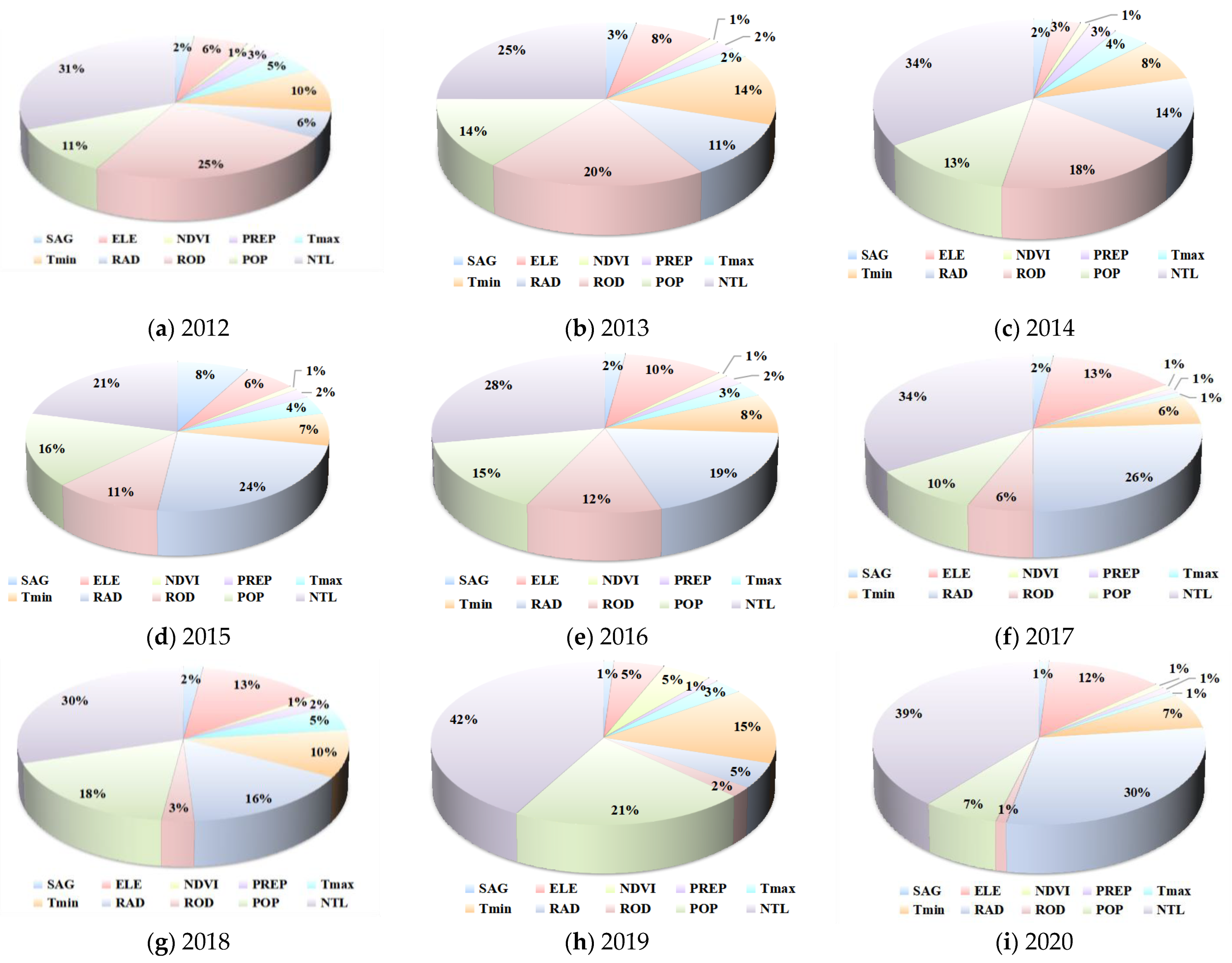
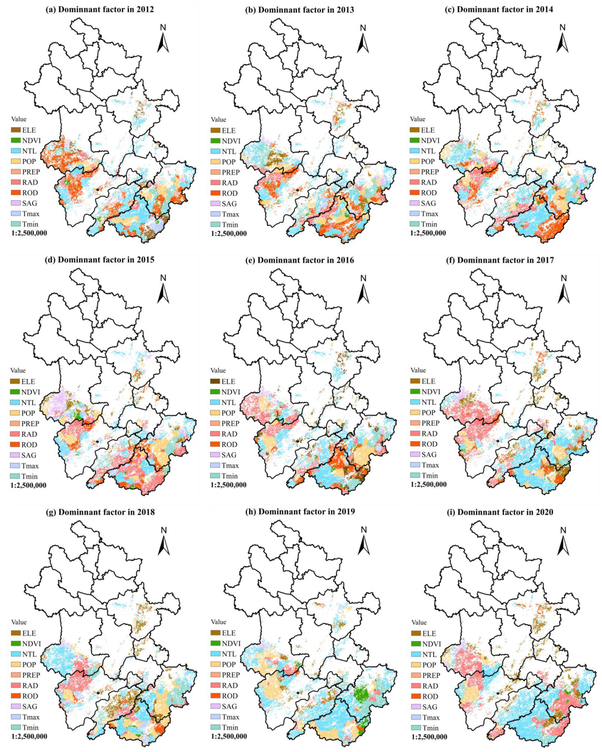
3.4. Spatiotemporal Analysis of Dominant Factors

In this study, the data we applied in the GTWR model were standardized, so the coefficients obtained were also standardized. Thus, the coefficients of each driving factor obtained by the GTWR model can reflect the relative importance of this factor in the occurrence of forest fires. We defined the driving factor with the most significant positive coefficient in each grid as the dominant factor for this grid, which contributes most to the occurrence of forest fires here. For visualization, we plotted the spatial and temporal distribution of the dominant factors and the pie chart of the spatial proportion of dominant factors for each year. The visualization results showed that there was also spatial and temporal heterogeneity in the distribution of the dominant factors.

The pie chart reveals that the dominant factors with more enormous spatial proportions were NTL, RAD, ROD, and POP (Figure 19). It is noteworthy that the spatial proportions of NTL were the largest among all factors in each year except 2015. The spatial proportion of POP, RAD, and NTL roughly showed an increasing trend during the study period, but the spatial proportion of ROD gradually decreased over time. The least spatially dominant factor was NDVI, and its spatial proportion remained almost constant during the study period. The spatial proportion of ELE showed a generally increasing trend over time, but it always remained at around 10%, similar to Tmin. The spatial proportions of SAG, PREP, and Tmax remained almost below 5%. We can also observe the annual spatial distribution of the dominant factors (Figure 20). From 2012 to 2014, the spatial dominance of ROD and NTL was relatively large. In these three years, ROD mainly dominated forest fires in Huangshan, Lu’an, and Anqing; NTL widely dominated forest fires in Chuzhou, Wuhu, Ma’anshan, Chizhou, and Huangshan. From 2015 to 2018, NTL and RAD spatially dominated forest fires in Chizhou, Huangshan, and Xuancheng; RAD dominated forest fires in Anqing, Chizhou, Huangshan, and Lu’an. From 2018 to 2020, the spatial dominance of RAD, NTL, and POP was relatively large. RAD mostly dominated forest fires in Lu’an, Anqing, and Xuancheng; NTL chiefly played a dominant role in forest fires in Lu’an, Chizhou, Huangshan, and Xuancheng; POP primarily dominated the occurrence of forest fires in Lu’an, Anqing, Xuancheng, and Huangshan. The spatial distribution revealed that RAD mainly dominated the occurrence of forest fires located on the edge of cities or the junction of adjacent cities. ROD mainly dominated forest fires located in the junctions of adjacent cities or the edges of forest areas near towns. The areas where POP dominated forest fire occurrence were mostly near ecotourism areas and tourist attractions. These findings are consistent with the actual situation. In some years, ELE exerted dominant effects on forest fires in Chuzhou, Ma’anshan, and Hefei. Meteorological factors such as Tmin and Tmax and vegetation factors NDVI dominated the occurrence of forest fires mainly in cities with large forest areas such as Xuancheng and Huangshan. Through the above analysis, we found that socioeconomic factors widely dominated forest fire occurrence in both spatial and temporal dimensions. Vegetation, topography, and meteorology played weaker dominant roles in forest fire occurrence in this study.

4. Discussion

4.1. Advantage of the GTWR Model

In recent years, many studies have used models such as GWR to study forest fire occurrence spatial patterns. Some studies have used statistical methods to explore the temporal patterns of forest fires. However, these studies always separated the temporal and spatial dimensions and conducted independent studies on forest fires’ spatial patterns or temporal patterns. In this study, we utilized the spatiotemporal coupling feature of the GTWR model to study the varying correlations between forest fires and driving factors in the temporal and spatial dimensions simultaneously. Therefore, compared with previous studies, this study can capture the differences in the correlations between driving factors and forest fires in the same year in different spatial locations and the variable trends in the correlations between driving factors and forest fires in the same spatial area in different years. In addition, the GTWR model can grab the abnormal changes in the correlated relationships with forest fires at corresponding spatiotemporal locations when the driving factors undergo abnormal changes. By considering spatiotemporal coupling, the GTWR model can deeply explore and explain the spatiotemporal heterogeneity of the correlations between driving factors and forest fires.

4.2. Main Findings

This study’s primary finding is that the driving factors’ effects on forest fires were spatiotemporally heterogeneous. At the provincial level, the spatiotemporal heterogeneity was mainly reflected in the changes in the spatial proportion of positive coefficients over time. The spatial distribution of correlation coefficients also revealed the spatial and temporal heterogeneity of forest fire occurrence by the differences in the spatial distribution of correlation coefficients between driving factors and forest fires from year to year. At the municipal level, spatiotemporal heterogeneity was mainly reflected in the fact that the correlations between driving factors and forest fires had different temporal variations in different cities. On the one hand, although the driving factors in different cities had similar temporal trends, the correlations between the driving factors and forest fires showed different temporal trends in different cities or similar temporal trends but with different degrees of change. For example, NTL had similar changes in Huangshan, Xuancheng, Anqing, and Hefei. However, the positive correlations between NTL and forest fires increased at different rates over time in Huangshan (Figure 8a) and Xuancheng (Figure 8a). They decreased at different rates over time in Anqing (Figure 8c) and Hefei (Figure 8d). The ROD of Chuzhou, Anqing, Xuancheng, and Chizhou all increased over time. The ROD coefficients of Chuzhou (Figure 14a) increased overall, while those of Anqing (Figure 14b), Xuancheng (Figure 14c), and Chizhou (Figure 14d) decreased over time. In addition, the fluctuations of PREP in the time dimension changed similarly in Chizhou, Xuancheng, Chuzhou, and Maanshan. Nevertheless, in Chizhou (Figure 16b) and Xuancheng (Figure 16c), forest fire occurrence was not sensitive to changes in mean PREP. Changes in mean PREP did not cause significant changes in mean PREP coefficients, which remained near zero in both cities. In Chuzhou (Figure 16a) and Ma’anshan (Figure 16d), forest fire occurrence was relatively sensitive to changes in mean PREP, with mean PREP increasing roughly over the study period and mean PREP coefficients decreasing roughly over the study period. On the other hand, the driving factors in different cities had different trends over time, and the correlated coefficients showed different trends. For example, POP in Anqing (Figure 10a) and Hefei (Figure 10b) increased over time during the study period, and the corresponding coefficients also had increasing trends. However, POP decreased generally, and POP coefficients decreased during the study period in Lu’an (Figure 10c).

We conjectured that the spatiotemporal heterogeneity in the relationships between factors and forest fires was caused by changes in the driving factors themselves in space and time on the one hand and by mutual checks and balances of the driving factors in the occurrence of forest fires on the other. It has been shown that climate was much less critical for forest fires where human social activities were more prominent in America [57], indicating human activities may not only influence the fire regimes and can override or mask the influence of climate. This same competitiveness exists between driving factors in our study, and when one factor was less important for forest fire occurrence, it may be that other factors were more critical for forest fire occurrence. For example, ROD increased with time in Anqing, Xuancheng, and Chizhou, but the ROD coefficient decreased. This is because the importance of ROD was weakened by the increase of other factors for forest fire occurrences in these cities, such as POP in Anqing (Figure 10a), NTL, and RAD in Xuancheng (Figure 18b and Figure 12a), and Tmax in Chizhou (Figure 18b).

4.3. Applicability of Nighttime Light

The contrast between light and dark areas on nighttime light remote sensing images makes it a powerful tool for studying human activities and their impacts. Since there is a positive correlation between light intensity and social economy, many studies have used this quantitative relationship to estimate socioeconomic factors, such as urbanization level estimation, population distribution estimation, GDP, energy consumption, and carbon emission. Since nighttime light remote sensing data were primarily used to estimate other socioeconomic factors reflecting human activities, it is better to consider nighttime light as one of the socioeconomic factors affecting forest fire occurrence. On the other hand, nighttime light can reflect information about traffic roads, residential areas, and other factors closely related to population or urban, and therefore can provide more comprehensive information. Therefore, this study innovatively introduced nighttime light as one socioeconomic factor that affects forest fires. The results showed that the spatial proportion of NTL positive coefficients exceeded 50% in eight out of nine years and showed a general increasing trend in the temporal dimension during the study period (Figure 7). From 2016 to 2020, the spatial proportions of NTL positive coefficients exceeded that of other factors (Figure 7). The spatial and temporal distribution diagram of NTL coefficients showed that the relationships between NTL and forest fires were mainly distinctly positive or extremely positive (Figure S2). In the analysis of dominant factors, the spatial areas where NTL dominates forest fires were the largest (Figure 19 and Figure 20). These results all suggest that nighttime light was closely related to forest fires and was significantly important in the occurrence of forest fires in Anhui in this study. It is reasonable and practical to take nighttime light as a factor potentially affecting the occurrence of forest fires.

4.4. Limitations and Outlooking

According to [35], it is better to consider fire size, season, and fire cause when investigating the relationships between fire occurrence and factors. Our study lost sight of these aspects of model construction and was not the best practice. We did not consider factors such as wind speed, air humidity, vegetation type, and soil moisture in selecting driving factors due to data availability. This study built a framework for assessing the spatiotemporal patterns of forest fire occurrence with the GTWR model. We explored the spatiotemporal heterogeneity of driving factors affecting forest fire occurrence by coupling their spatiotemporal information. This study improved the interpretation of forest fire occurrence, filled a crucial gap in forest fire research, and provided unique insights into studying spatiotemporal patterns of forest fire occurrence. We successfully applied this framework to study interannual forest fire occurrence patterns at the regional scale in China. Future studies can be conducted at finer temporal and broader spatial scales to understand and reveal the patterns of forest fire occurrence in other places. In recent years, China has made great efforts to build forest cities, and the boundary between forest and city has been blurred and gradually integrated. The influence of cities on forests is becoming increasingly non-negligible. Hence, future research needs to consider the relationships between urban development or human activities and forest fire occurrence in China. This study innovatively introduced nighttime light as a socioeconomic factor, so future research can try to use more factors with high spatial and temporal resolutions like this instead of traditional socioeconomic factors with low spatial and temporal resolutions to improve the accuracy of research results.

5. Conclusions

Identifying the driving factors and exploring the spatiotemporal patterns of forest fire occurrence is crucial for forest fire management decision-making. In this study, we applied the GTWR model to investigate the spatiotemporal patterns of forest fire occurrence in the Anhui province from 2012 to 2020. We selected factors representing topography, vegetation, meteorology, and social economy as independent variables and the number of forest fires as the dependent variable. In acquiring data, we employed remote sensing data for forest fire data, nighttime light, normalized difference vegetation index, and topographic factors in this study. We carried out the spatial autocorrelation test for forest fires in Anhui. The results showed a spatial autocorrelation of forest fires in Anhui from 2012 to 2020, with high-high aggregation of forest fires in eastern cities, including Ma’anshan, Wuhu, Tongling, and Xuancheng. We compared the performance of the OLS model, the GWR model, and the GTWR model using the same dataset. The GTWR model outperformed the other two, and the OLS model performed the worst, implying the necessity of considering temporal heterogeneity in addition to spatial heterogeneity in the forest fire occurrence study. Based on the results of the GTWR model, we carried out the spatiotemporal analysis of the relationship between each driving factor and forest fires, as well as dominant factors. Socioeconomic factors were most strongly correlated with forest fires in Anhui province during the study period, while vegetation, topography, and meteorology were less correlated with forest fires. The positive effects of socioeconomic factors on forest fire occurrence were relatively extensive and robust in the spatial and temporal dimensions. The areas where population density, railway density, and nighttime light positively impacted had an overall tendency to expand over time. The spatiotemporal analysis of the dominant factors indicated that forest fire occurrence in Anhui province was mainly dominated by socioeconomic factors, while the dominant role of vegetation, topography, and meteorology was relatively limited. Socioeconomic factors, including nighttime light, railway density, road density, and population density, widely dominated the occurrence of forest fires in the Anhui province. It is worth noting that nighttime light played the most extensive dominant role in forest fires in Anhui province in the spatial and temporal dimensions, so it is reasonable and practical to take nighttime light as one of the influencing factors. The forest areas where population density, railway density, and nighttime light dominated fire occurrence tended to expand over time. Therefore, it is recommended that the Anhui province should strengthen the monitoring and prevention of forest fires in forest scenic areas with strong social activities.

This study innovatively introduced nighttime light as a driving factor of forest fires, which provides a reference for selecting future socioeconomic factors of forest fires. This study built a framework for exploring the spatiotemporal patterns of forest fire occurrence with the GTWR model. By coupling the spatiotemporal information of driving factors and forest fires in the model, we not only grabbed the varying spatial relationship between the driving factors and forest fire but also captured the temporal variation patterns corresponding to the correlation coefficients and driving factors. We also identified the dominant factors from the spatiotemporal dimension. Therefore, this framework can help explore the spatiotemporal heterogeneity of forest fire occurrence fully. This study improved the level of explanation for forest fire occurrence, providing unique insights into studying spatiotemporal patterns of forest fires. This work will contribute to understanding the driving factors of forest fires in Anhui at the provincial level and help policymakers develop fire management strategies and allocate resources rationally to reduce potential fire hazards.

References

1. Miranda, B.R.; Sturtevant, B.R.; Stewart, S.I.; Hammer, R.B. Spatial and temporal drivers of wildfire occurrence in the context of rural development in northern Wisconsin, USA. Int. J. Wildland Fire 2011, 21, 141–154. [Google Scholar] [CrossRef]
2. Nunes, A.; Lourenço, L.; Meira, A.C. Exploring spatial patterns and drivers of forest fires in Portugal (1980–2014). Sci. Total Environ. 2016, 573, 1190–1202. [Google Scholar] [CrossRef] [PubMed]
3. Trang, P.; Andrew, M.; Chu, T.; Enright, N. Forest fire and its key drivers in the tropical forests of northern Vietnam. Int. J. Wildland Fire 2022, 31, 213–229. [Google Scholar] [CrossRef]
4. Adab, H.; Kanniah, K.D.; Solaimani, K. Modeling forest fire risk in the northeast of Iran using remote sensing and GIS techniques. Nat. Hazards 2013, 65, 1723–1743. [Google Scholar] [CrossRef]
5. Pourtaghi, Z.S.; Pourghasemi, H.R.; Aretano, R.; Semeraro, T. Investigation of general indicators influencing on forest fire and its susceptibility modeling using different data mining techniques. Ecol. Indic. 2016, 64, 72–84. [Google Scholar] [CrossRef]
6. Huesca, M.; Litago, J.; Palacios-Orueta, A.; Montes, F.; Sebastián-López, A.; Escribano, P. Assessment of forest fire seasonality using MODIS fire potential: A time series approach. Agric. For. Meteorol. 2009, 149, 1946–1955. [Google Scholar] [CrossRef]
7. Hong, H.; Tsangaratos, P.; Ilia, I.; Liu, J.; Zhu, A.-X.; Xu, C. Applying genetic algorithms to set the optimal combination of forest fire related variables and model forest fire susceptibility based on data mining models. The case of Dayu County, China. Sci. Total Environ. 2018, 630, 1044–1056. [Google Scholar] [CrossRef]
8. Janiec, P.; Gadal, S. A comparison of two machine learning classification methods for remote sensing predictive modeling of the forest fire in the North-Eastern Siberia. Remote Sens. 2020, 12, 4157. [Google Scholar] [CrossRef]
9. Kim, T.; Hwang, S.; Choi, J. Characteristics of spatiotemporal changes in the occurrence of forest fires. Remote Sens. 2021, 13, 4940. [Google Scholar] [CrossRef]
10. Li, W.; Li, P.; Feng, Z. Delineating Fire-Hazardous Areas and Fire-Induced Patterns Based on Visible Infrared Imaging Radiometer Suite (VIIRS) Active Fires in Northeast China. Remote Sens. 2022, 14, 5115. [Google Scholar] [CrossRef]
11. Ge, X.; Yang, Y.; Peng, L.; Chen, L.; Li, W.; Zhang, W.; Chen, J. Spatio-temporal knowledge graph based forest fire prediction with multi source heterogeneous data. Remote Sens. 2022, 14, 3496. [Google Scholar] [CrossRef]
12. Sulova, A.; Jokar Arsanjani, J. Exploratory analysis of driving force of wildfires in Australia: An application of machine learning within Google Earth engine. Remote Sens. 2020, 13, 10. [Google Scholar] [CrossRef]
13. Oliveira, S.; Oehler, F.; San-Miguel-Ayanz, J.; Camia, A.; Pereira, J.M. Modeling spatial patterns of fire occurrence in Mediterranean Europe using Multiple Regression and Random Forest. For. Ecol. Manag. 2012, 275, 117–129. [Google Scholar] [CrossRef]
14. Kim, S.J.; Lim, C.-H.; Kim, G.S.; Lee, J.; Geiger, T.; Rahmati, O.; Son, Y.; Lee, W.-K. Multi-temporal analysis of forest fire probability using socio-economic and environmental variables. Remote Sens. 2019, 11, 86. [Google Scholar] [CrossRef] [Green Version]
15. Monjarás-Vega, N.A.; Briones-Herrera, C.I.; Vega-Nieva, D.J.; Calleros-Flores, E.; Corral-Rivas, J.J.; López-Serrano, P.M.; Pompa-García, M.; Rodríguez-Trejo, D.A.; Carrillo-Parra, A.; González-Cabán, A. Predicting forest fire kernel density at multiple scales with geographically weighted regression in Mexico. Sci. Total Environ. 2020, 718, 137313. [Google Scholar] [CrossRef] [PubMed]
16. Xiong, Q.; Luo, X.; Liang, P.; Xiao, Y.; Xiao, Q.; Sun, H.; Pan, K.; Wang, L.; Li, L.; Pang, X. Fire from policy, human interventions, or biophysical factors? Temporal–spatial patterns of forest fire in southwestern China. For. Ecol. Manag. 2020, 474, 118381. [Google Scholar] [CrossRef]
17. Bar, S.; Parida, B.R.; Roberts, G.; Pandey, A.C.; Acharya, P.; Dash, J. Spatio-temporal characterization of landscape fire in relation to anthropogenic activity and climatic variability over the Western Himalaya, India. GIScience Remote Sens. 2021, 58, 281–299. [Google Scholar] [CrossRef]
18. Widayati, A.; Jones, S.; Carlisle, B. Accessibility factors and conservation forest designation affecting rattan cane harvesting in Lambusango Forest, Buton, Indonesia. Hum. Ecol. 2010, 38, 731–746. [Google Scholar] [CrossRef]
19. Bui, D.T.; Bui, Q.-T.; Nguyen, Q.-P.; Pradhan, B.; Nampak, H.; Trinh, P.T. A hybrid artificial intelligence approach using GIS-based neural-fuzzy inference system and particle swarm optimization for forest fire susceptibility modeling at a tropical area. Agric. For. Meteorol. 2017, 233, 32–44. [Google Scholar] [CrossRef]
20. Bui, D.T.; Hoang, N.-D.; Samui, P. Spatial pattern analysis and prediction of forest fire using new machine learning approach of Multivariate Adaptive Regression Splines and Differential Flower Pollination optimization: A case study at Lao Cai province (Viet Nam). J. Environ. Manag. 2019, 237, 476–487. [Google Scholar] [CrossRef]
21. Syphard, A.D.; Radeloff, V.C.; Keeley, J.E.; Hawbaker, T.J.; Clayton, M.K.; Stewart, S.I.; Hammer, R.B. Human influence on California fire regimes. Ecol. Appl. 2007, 17, 1388–1402. [Google Scholar] [CrossRef] [PubMed]
22. Martínez, J.; Vega-Garcia, C.; Chuvieco, E. Human-caused wildfire risk rating for prevention planning in Spain. J. Environ. Manag. 2009, 90, 1241–1252. [Google Scholar] [CrossRef] [PubMed]
23. Zhang, H.; Han, X.; Dai, S. Fire occurrence probability mapping of northeast China with binary logistic regression model. IEEE J. Sel. Top. Appl. Earth Obs. Remote Sens. 2013, 6, 121–127. [Google Scholar] [CrossRef]
24. Oliveira, S.; Pereira, J.M.; San-Miguel-Ayanz, J.; Lourenço, L. Exploring the spatial patterns of fire density in Southern Europe using Geographically Weighted Regression. Appl. Geogr. 2014, 51, 143–157. [Google Scholar] [CrossRef]
25. Su, Z.; Hu, H.; Wang, G.; Ma, Y.; Yang, X.; Guo, F. Using GIS and Random Forests to identify fire drivers in a forest city, Yichun, China. Geomat. Nat. Hazards Risk 2018, 9, 1207–1229. [Google Scholar] [CrossRef] [Green Version]
26. Zapata-Ríos, X.; Lopez-Fabara, C.; Navarrete, A.; Torres-Paguay, S.; Flores, M. Spatiotemporal patterns of burned areas, fire drivers, and fire probability across the equatorial Andes. J. Mt. Sci. 2021, 18, 952–972. [Google Scholar] [CrossRef]
27. Guo, F.; Su, Z.; Wang, G.; Sun, L.; Lin, F.; Liu, A. Wildfire ignition in the forests of southeast China: Identifying drivers and spatial distribution to predict wildfire likelihood. Appl. Geogr. 2016, 66, 12–21. [Google Scholar] [CrossRef]
28. Xu, X. 1 km GDP Spatial Distribution Grid Dataset for China. Available online: https://www.resdc.cn/DOI/DOI.aspx?DOIID=33 (accessed on 1 December 2022).
29. Zhang, X.; Wu, J.; Peng, J.; Cao, Q. The uncertainty of nighttime light data in estimating carbon dioxide emissions in China: A comparison between DMSP-OLS and NPP-VIIRS. Remote Sens. 2017, 9, 797. [Google Scholar] [CrossRef] [Green Version]
30. Zhao, M.; Cheng, W.; Zhou, C.; Li, M.; Huang, K.; Wang, N. Assessing spatiotemporal characteristics of urbanization dynamics in Southeast Asia using time series of DMSP/OLS nighttime light data. Remote Sens. 2018, 10, 47. [Google Scholar] [CrossRef] [Green Version]
31. Jiang, Z.; Zhai, W.; Meng, X.; Long, Y. Identifying shrinking cities with NPP-VIIRS nightlight data in China. J. Urban Plan. Dev. 2020, 146, 04020034. [Google Scholar] [CrossRef]
32. Eskandari, S.; Miesel, J.R.; Pourghasemi, H.R. The temporal and spatial relationships between climatic parameters and fire occurrence in northeastern Iran. Ecol. Indic. 2020, 118, 106720. [Google Scholar] [CrossRef]
33. Pang, Y.; Li, Y.; Feng, Z.; Feng, Z.; Zhao, Z.; Chen, S.; Zhang, H. Forest Fire Occurrence Prediction in China Based on Machine Learning Methods. Remote Sens. 2022, 14, 5546. [Google Scholar] [CrossRef]
34. Sun, Y.; Zhang, F.; Lin, H.; Xu, S. A Forest Fire Susceptibility Modeling Approach Based on Light Gradient Boosting Machine Algorithm. Remote Sens. 2022, 14, 4362. [Google Scholar] [CrossRef]
35. Rodrigues, M.; Jiménez-Ruano, A.; Peña-Angulo, D.; De la Riva, J. A comprehensive spatial-temporal analysis of driving factors of human-caused wildfires in Spain using Geographically Weighted Logistic Regression. J. Environ. Manag. 2018, 225, 177–192. [Google Scholar] [CrossRef] [Green Version]
36. Cimdins, R.; Krasovskiy, A.; Kraxner, F. Regional Variability and Driving Forces behind Forest Fires in Sweden. Remote Sens. 2022, 14, 5826. [Google Scholar] [CrossRef]
37. Huang, B.; Wu, B.; Barry, M. Geographically and temporally weighted regression for modeling spatio-temporal variation in house prices. Int. J. Geogr. Inf. Sci. 2010, 24, 383–401. [Google Scholar] [CrossRef]
38. Wu, B.; Li, R.; Huang, B. A geographically and temporally weighted autoregressive model with application to housing prices. Int. J. Geogr. Inf. Sci. 2014, 28, 1186–1204. [Google Scholar] [CrossRef]
39. Fotheringham, A.S.; Crespo, R.; Yao, J. Geographical and temporal weighted regression (GTWR). Geogr. Anal. 2015, 47, 431–452. [Google Scholar] [CrossRef] [Green Version]
40. Cui, L.; Li, R.; Zhang, Y.; Meng, Y.; Zhao, Y.; Fu, H. A geographically and temporally weighted regression model for assessing intra-urban variability of volatile organic compounds (VOCs) in Yangpu district, Shanghai. Atmos. Environ. 2019, 213, 746–756. [Google Scholar] [CrossRef]
41. Abedi Gheshlaghi, H. Using GIS to develop a model for forest fire risk mapping. J. Indian Soc. Remote Sens. 2019, 47, 1173–1185. [Google Scholar] [CrossRef]
42. Jaafari, A.; Zenner, E.K.; Panahi, M.; Shahabi, H. Hybrid artificial intelligence models based on a neuro-fuzzy system and metaheuristic optimization algorithms for spatial prediction of wildfire probability. Agric. For. Meteorol. 2019, 266, 198–207. [Google Scholar] [CrossRef]
43. Murthy, K.K.; Sinha, S.K.; Kaul, R.; Vaidyanathan, S. A fine-scale state-space model to understand drivers of forest fires in the Himalayan foothills. For. Ecol. Manag. 2019, 432, 902–911. [Google Scholar] [CrossRef]
44. Nami, M.; Jaafari, A.; Fallah, M.; Nabiuni, S. Spatial prediction of wildfire probability in the Hyrcanian ecoregion using evidential belief function model and GIS. Int. J. Environ. Sci. Technol. 2018, 15, 373–384. [Google Scholar] [CrossRef]
45. Zhao, P.; Zhang, F.; Lin, H.; Xu, S. GIS-Based Forest Fire Risk Model: A Case Study in Laoshan National Forest Park, Nanjing. Remote Sens. 2021, 13, 3704. [Google Scholar] [CrossRef]
46. Valdez, M.C.; Chang, K.-T.; Chen, C.-F.; Chiang, S.-H.; Santos, J.L. Modelling the spatial variability of wildfire susceptibility in Honduras using remote sensing and geographical information systems. Geomat. Nat. Hazards Risk 2017, 8, 876–892. [Google Scholar] [CrossRef] [Green Version]
47. Valente, F.; Laurini, M. Spatio-temporal analysis of fire occurrence in Australia. Stoch. Environ. Res. Risk Assess. 2021, 35, 1759–1770. [Google Scholar] [CrossRef]
48. Xu, X. Spatial Distribution Dataset of China Annual Vegetation Index (NDVI). Available online: https://www.resdc.cn/DOI/DOI.aspx?DOIID=49 (accessed on 1 December 2022).
49. Zhao, B.; Mao, K.; Cai, Y.; Shi, J.; Li, Z.; Qin, Z.; Meng, X.; Shen, X.; Guo, Z. A combined Terra and Aqua MODIS land surface temperature and meteorological station data product for China from 2003 to 2017. Earth Syst. Sci. Data 2020, 12, 2555–2577. [Google Scholar] [CrossRef]
50. National Earth System Science Data Center. Available online: http://www.geodata.cn (accessed on 1 December 2022).
51. Peng, S.; Ding, Y.; Liu, W.; Li, Z. 1 km monthly temperature and precipitation dataset for China from 1901 to 2017. Earth Syst. Sci. Data 2019, 11, 1931–1946. [Google Scholar] [CrossRef] [Green Version]
52. Abdi, O.; Kamkar, B.; Shirvani, Z.; Teixeira da Silva, J.A.; Buchroithner, M.F. Spatial-statistical analysis of factors determining forest fires: A case study from Golestan, Northeast Iran. Geomat. Nat. Hazards Risk 2018, 9, 267–280. [Google Scholar] [CrossRef] [Green Version]
53. Tariq, A.; Shu, H.; Siddiqui, S.; Munir, I.; Sharifi, A.; Li, Q.; Lu, L. Spatio-temporal analysis of forest fire events in the Margalla Hills, Islamabad, Pakistan using socio-economic and environmental variable data with machine learning methods. J. For. Res. 2021, 33, 183–194. [Google Scholar] [CrossRef]
54. Guo, F.; Su, Z.; Tigabu, M.; Yang, X.; Lin, F.; Liang, H.; Wang, G. Spatial modelling of fire drivers in urban-forest ecosystems in China. Forests 2017, 8, 180. [Google Scholar] [CrossRef] [Green Version]
55. Nikhil, S.; Danumah, J.H.; Saha, S.; Prasad, M.K.; Rajaneesh, A.; Mammen, P.C.; Ajin, R.; Kuriakose, S.L. Application of GIS and AHP Method in Forest Fire Risk Zone Mapping: A Study of the Parambikulam Tiger Reserve, Kerala, India. J. Geovisualization Spat. Anal. 2021, 5, 14. [Google Scholar] [CrossRef]
56. Moran, P.A. Notes on continuous stochastic phenomena. Biometrika 1950, 37, 17–23. [Google Scholar] [CrossRef] [PubMed]
57. Syphard, A.D.; Keeley, J.E.; Pfaff, A.H.; Ferschweiler, K. Human presence diminishes the importance of climate in driving fire activity across the United States. Proc. Natl. Acad. Sci. USA 2017, 114, 13750–13755. [Google Scholar] [CrossRef] [PubMed]
Figure 1. Location of the study area (Anhui province).
Remotesensing 15 00598 g001
Figure 2. Data processing workflows.
Remotesensing 15 00598 g002
Figure 3. Spatial distribution of forest fire points in Anhui during 2012–2020.
Remotesensing 15 00598 g003
Figure 4. The LISA maps from 2012 to 2020.
Remotesensing 15 00598 g004
Figure 5. Temporal trends of mean NDVI values and spatial proportion of positive NDVI coefficients.
Remotesensing 15 00598 g005
Figure 6. Temporal trends of mean NDVI values and mean NDVI coefficients in (a) Xuancheng and (b) Ma’anshan.
Remotesensing 15 00598 g006
Figure 7. Temporal trends of mean NTL values and spatial proportion of positive NTL coefficients.
Remotesensing 15 00598 g007
Figure 8. Temporal trends of mean NTL values and mean NTL coefficients in (a) Huangshan; (b) Xuancheng; (c) Anqing; (d) Hefei.
Remotesensing 15 00598 g008
Figure 9. Temporal trends of mean POP values and spatial proportion of positive POP coefficients.
Remotesensing 15 00598 g009
Figure 10. Temporal trends of mean POP values and mean POP coefficients in (a) Anqing; (b) Hefei; (c) Lu’an.
Remotesensing 15 00598 g010
Figure 11. Temporal trends of mean RAD values and spatial proportion of positive RAD coefficients.
Remotesensing 15 00598 g011
Figure 12. Temporal trends of mean RAD values and mean RAD coefficients in (a) Xuancheng; (b) Anqing; (c) Huangshan; (d) Anqing.
Remotesensing 15 00598 g012
Figure 13. Temporal trends of mean ROD values and spatial proportion of positive ROD coefficients.
Remotesensing 15 00598 g013
Figure 14. Temporal trends of mean ROD values and mean ROD coefficients in (a) Chuzhou; (b) Anqing; (c) Xuancheng; (d) Chizhou.
Remotesensing 15 00598 g014
Figure 15. Temporal trends of mean PREP values and spatial proportion of positive PREP coefficients.
Remotesensing 15 00598 g015
Figure 16. Temporal trends of mean PREP values and mean PREP coefficients in (a) Chuzhou; (b) Chizhou; (c) Xuancheng; (d) Ma’anshan.
Remotesensing 15 00598 g016
Figure 17. Temporal trends of mean Tmax values and mean Tmax coefficients in (a) Lu’an; (b) Chizhou.
Remotesensing 15 00598 g017
Figure 18. Temporal trends of mean Tmin values and spatial proportion of positive Tmin coefficients.
Remotesensing 15 00598 g018
Figure 19. Spatial proportion of dominant factors from (a) 2012 to (i) 2020.
Remotesensing 15 00598 g019
Figure 20. Spatial distribution of dominant factors from 2012 to 2020.
Remotesensing 15 00598 g020