Assessing the Vertical Structure of Forests Using Airborne and Spaceborne LiDAR Data in the Austrian Alps

Abstract

Vertical structure is an important parameter not only for assessment of the naturalness of a forest and several functional parameters, such as biodiversity or protection from avalanches or rockfall, but also for estimating biomass/carbon content. This study analyses the options for assessing vertical forest structure by using airborne (ALS) and spaceborne LiDAR data (GEDI) in a mountainous near-natural forest in the Austrian Alps. Use of the GEDI waveform data (L1B) is still heavily underexploited for vertical forest structure assessments. Two indicators for explaining forest vertical structure are investigated in this study: foliage height diversity (FHD) and number of layers (NoL). For estimation of NoL, two different approaches were tested: break-detection algorithm (BDA) and expert-based assessment (EBA). The results showed that FHD can be used to separate three structural classes; separability is only slightly better for ALS than for GEDI data on a 25 m diameter plot level. For NoL, EBA clearly outperformed BDA in terms of overall accuracy (OA) by almost 20%. A better OA for NoL was achieved using ALS (49.5%) rather than GEDI data (44.2%). In general, OA is limited by difficult terrain and near-natural forests with high vertical structure. The usability of waveform-based structure parameters is, nonetheless, promising and should be further tested on larger areas, including managed forests and simpler stands.

1. Introduction

Forests have become a focal point for their role in the global carbon cycle [1] in the frame of climate change. The vertical structure of a forest is—along with its canopy height—a significant parameter for assessing biomass [2] and, thus, also carbon content. In general, the magnitude of a forest’s contribution as a carbon sink is not yet fully understood and remains uncertain [3]. Therefore, attempts to better understand and map vertical forest structure also contribute to improved carbon content modelling. Since the 1960s, forest structure (also termed as diversity, heterogeneity or complexity [4]) has been discussed in forest science as an important parameter for assessing temporal dynamics, such as gaps and regeneration [5], for forest management [6] and biodiversity issues [7]. Anthropogenic activities not only affect the role of the forests as carbon storage but are also a threat to biodiversity [8]. Due to human-induced climate change, biodiversity is rapidly declining and habitats are being destroyed [9,10]. In order to address all these effects on the ecosystem, continuous spatial measurement frameworks for land cover, vegetation and forest parameters are needed [11].

Early endeavours for quantifying forest variables—including forest structure—relied mainly on in situ techniques, hence limiting the spatial and temporal extent of data. Introduction of remote sensing technologies moved beyond these constraints by enabling transferability to the required resolution to detect changes in forest structures even over large and remote areas. Several forest parameters are currently obtained by remote sensing methods in an operational manner, such as the main tree species or canopy cover—which are available within Europe’s COPERNICUS program—understood as “high-resolution layers” [12,13]. Three-dimensional parameters, such as canopy height, biomass content or vertical structure, have until recently been limited to analysis of airborne laser scanning (ALS), which is still costly in terms of acquisition and, therefore, limited in spatial coverage and temporal updates. Only within the last two years and thanks to the availability of spaceborne laser scanning (SLS) data has this situation changed, and large-area forest canopy height maps have also been produced [14,15]. From past and existing spaceborne laser scanners, such as Ice, Cloud, and Land Elevation Satellite (ICESAT), Cloud-Aerosol LiDAR and Infrared Pathfinder Satellite Observation (CALIPSO), Atmospheric Dynamics Mission-Aeolus (ADM-AEOLUS) and ICESAT-2, only the Global Ecosystem Dynamics Investigation (GEDI) sensor is specifically designed for mapping vegetation and forest parameters [16]. We, therefore, limit our analysis to GEDI data, although we are aware of several papers having also used other SLS data for forest parameter assessments [17,18,19]. For GEDI, pre-launch calibration and validation studies employing simulated GEDI waveforms processed from ALS instruments show promising results and suggest that GEDI data are well suited for capturing vegetation patterns and biomass products [20,21,22,23]. Since the release of version 1 GEDI data, various studies have been published that assess accuracy of GEDI data by evaluating ground elevation and canopy height estimates against ALS height data [14,15,24,25]. These studies are in good agreement with each other and highlight the applicability of GEDI data to forest structure investigations.

The basic ability of a spaceborne laser to analyse complex forest structures with dense and multi-layered canopies enables not only canopy height and biomass estimations but also provides new and valuable insights into forest structure and biodiversity [25,26] and improves understanding of ecological functions [21]. From a literature review of 98 publicly available peer-reviewed studies, approximately two-thirds of the studies use GEDI data for assessing canopy height and profile metrics (level 2) as well as biomass estimates (level 4). From the remaining GEDI-related publications, only 30 made use of L1B waveforms. Of these, eighteen focussed on simulated L1B waveforms, twelve used real L1B data and one used both. Of these, most targeted the geolocation issue, e.g., by analysing water bodies (four publications) and canopy height and/or making comparisons with simulated waveforms. Dwiputra et al. [27] used waveforms to identify different vegetation types, whereas Liu et al. [28] aimed to improve canopy height estimations by employing waveform data. Nonetheless, geolocated waveforms (L1B) remain significantly under-exploited for assessing forest structure. Our study aims to contribute to filling this gap by using real L1B products and comparing them to ALS data for assessment of vertical forest structure. However, this aim is hampered because “vertical structure” or “forest structure” are rather ambiguous terms in forest science. The approaches to assess forest structure can be divided into three groups. First, many foresters consider diameter size distribution of trees (diameter at breast height—DBH) [29,30,31] as a parameter for defining vertical structure. The DBH distribution cannot be measured by ALS or SLS as this is not feasible from above. Only terrestrial manual measurements (with a measuring “kluppe”) or terrestrial laser scanning can measure DBH directly [32,33].

The second group of approaches use the height distribution of individual trees [34,35,36,37,38] to assess a forest’s structure. Dominant tree heights can be measured very accurately from ALS data, while results show lower accuracies for suppressed trees, e.g., in near-natural forests and/or complex stands [36,39,40,41].

Third, there are attempts to model the vertical structure not on an individual tree level but using an area-based approach, often also based upon ALS data. Some of these approaches use machine- or deep learning methods in a black-box approach [42,43]. Others rely on simpler statistical features [36,40,44,45,46] or expert/rule-based classification systems [37,47]. Among the latter, there is also a rather old approach called foliage height diversity (FHD) [7], which has been implemented in the GEDI processing chain of L1B data [21].

In our study, we will answer the following three research questions:

• How well are LiDAR data in general suitable for explaining vertical forest structure and the number of layers (NoL) in a near-natural mountainous forest?
• How well are GEDI data specifically suited for this purpose?
• What waveform-based indicators are best suited for explaining vertical forest structure?

2. Materials and Methods

2.1. Materials

2.1.1. Study Area

The study area (see Figure 1) is located in the central region of Austria and covers large parts of the National Park “Kalkalpen” forest. The park is located in the north-eastern Limestone Alps, characterised by very steep slopes ranging from 385 to 1963 m in elevation and a large shared area of forest and shrub vegetation cover (about 81% of the park) [48]. Selection of the study area is based upon three main reasons: first, availability of ALS data in close temporal proximity (2018) with the available GEDI data (2019–2020), which is necessary for comparison. The second reason is related to availability of old-growth beech forests, which have been designated as UNESCO World Heritage sites [49]. These forests, up to an elevation of 1450 m mainly beech and spruce–fir–beech forests, make up a climax vegetation community [48] and are supposedly highly structured and, therefore, an ideal testbed. 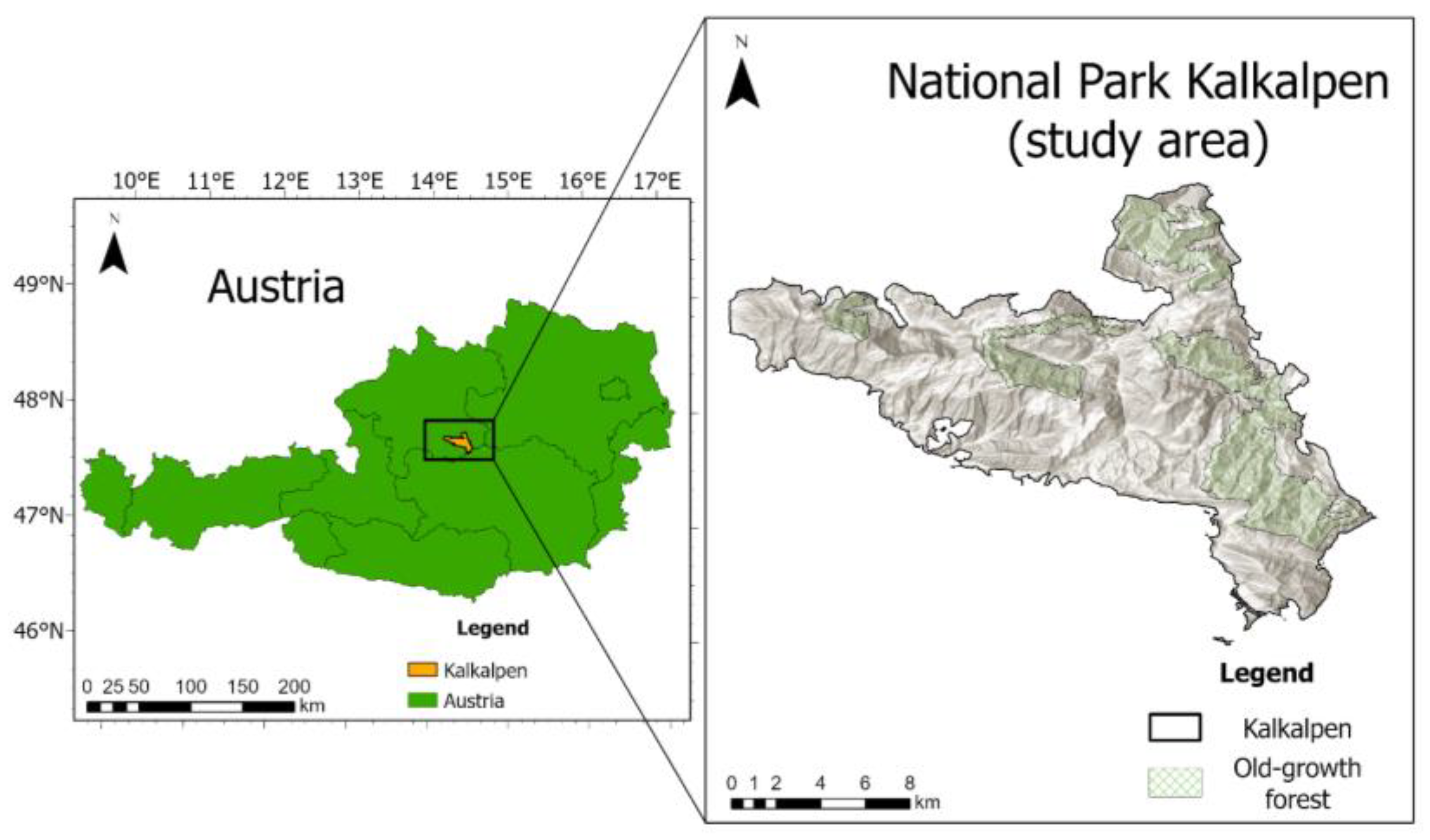Third, we want to test the usability of GEDI data in difficult, mountainous conditions characterised by steep slopes, small-structured alpine topography and complex terrain, and these characteristics are observed within the study area.

2.1.2. GEDI Data

The GEDI instrument is a space-borne LiDAR aboard the International Space Station, acquiring pointwise 3D data between 51.6°N and 51.6°S since April 2019. The LiDAR system is equipped with three lasers that are split into four beams and dithered into eight tracks that are 600 m apart. At every 60 m along the track, the instrument collects data of individual shots with a diameter of approximately 25 m on the ground. The delayed return energy is used to calculate the raw waveform (Level 1A–L1A) of the footprint.

With information from GEDI’s GPS and star trackers, the raw waveforms are geolocated and smoothed to form Level 1B data (L1B). Subsequently, they are processed as higher-level products, such as canopy height and profile metrics (L2 and L3) and biomass (L4) on footprint as well as on a gridded level. A detailed description of the data products can be found in [16], and data can be accessed via the Land Processes Distributed Active Archive Center (LP DAAC: https://lpdaac.usgs.gov/, accessed on 21 January 2023). In our study, we used L1B and L2B data.

L2B data provide information about a forest’s structure, such as canopy cover, plant area index (PAI) and FHD. GEDI’s canopy cover is defined as “the percent of the ground covered by the vertical projection of canopy material (i.e., leaves, branches and stems)” [50], which is slightly different from the crown cover’s definition that is commonly used in ALS data. Based on the canopy cover and the canopy’s directional gap probability (its complement), the plant area index (PAI) is calculated. Furthermore, the PAI is used to derive the FHD. A high FHD value indicates a more complex canopy structure [23].

2.1.3. ALS

ALS data were acquired on 21 May 2018 using an ultra-light airplane at a cruising altitude of ca. 790 m above ground. The sensor is a RIEGL VQ580 with a point density of >16 points/m². Additionally, true-colour and near-infrared imagery were acquired for visual comparison. Altogether, an area of approximately 4000 ha was covered by 50 flight lines.

2.2. Methods

The overall workflow used in this study is outlined in Figure 2. It comprises four main steps: pre-processing, indicator calculation, reference data generation and, finally, an evaluation of the results. Steps one to three are explained in the subsections of this chapter, and results of the evaluation are provided in Chapter 3.

2.2.1. Pre-Processing

Direct georeferencing is carried out for ALS by using a GPS/IMU unit: Novatel SPAN-FSAS [51]. Afterward, the resulting data were compared to existing data from a previous region-wide ALS campaign to ensure location accuracy. For GEDI, the given plot locations, as provided by the LP-DAAC were used in the initial step.

Furthermore, ALS point clouds are extracted for the given GEDI position in a 25 m diameter circle. Additionally, discrete LiDAR returns per 1 m vertical height layer are used to generate a “pseudo-waveform”. In full awareness of the difference, we use the term “waveform” for both the real GEDI waveform and the ALS pseudo-waveform in this publication. The comparison between the ALS waveform and the GEDI waveform, in many cases, reveals significant differences in the vertical profile (see Figure A1b,d,f in Appendix A). One potential reason for such differences is the geolocation of the GEDI footprints. According to GEDI documentation, “GEDI uses its own Global Positioning System (GPS), Inertial Measurement Unit (IMU), and information from three star trackers that permit GEDI to georeference each laser pulse to within 10 m (1 σ) (i.e. assuming a distribution of geolocation errors whose mean is zero, and whose standard deviation is 10 m) on the Earth’s surface” [16]. The effects of this geolocation error have been studied with respect to ground height [52], canopy height [52,53] and biomass [49,50]. It is evident that the geolocation error is the highest in areas with strong topography [54] and in forests with fragmented and heterogeneous canopies [53]. Both characteristics are present in our study area. Therefore, the correlation method of Blair and Hofton [55] implemented in the GEDI simulator [56] is used to test geolocation improvements. The basic idea of this approach is to create simulated waveforms for each GEDI orbit intersecting the ALS reference data. Subsequently, the offset that maximises the correlation between the measured GEDI waveform and the simulated (ALS-based) waveform is applied to all footprints of the corresponding orbit. The maximum deviation is set to 10 m in both x and y directions based on the value given in [16].

Additionally, from a total of 9065 footprints, only the GEDI footprints fulfilling the following requirements were included in the analysis. For each applied filter, the remaining footprints are provided in brackets:

• Quality flag = 1 (4618);
• Waveforms with terrain height within accuracy limits. Due to the steep terrain, inaccuracies with respect to the terrain’s height occur. In order not to impact the analysis, these outliers (>2*stdv) were discarded from further analysis (4174);
• Acquisition during leaf-on season (June–October 2019 and 2020) (2911);
• Degrade flag = 0 (2911);
• Data overlapping the ALS coverage (1734);
• Within areas, where no changes between 2018 and 2020 occurred (1725);
• Footprints, where GEDI or ALS estimate heights above ground of 50 m or more, are removed to account for artefacts (e.g., from birds) (1692).

For the remaining 1692 GEDI footprints, we recalculated the continuous waveforms of both ALS and GEDI into discrete 1 m height layers. Before moving on to indicator calculations, only for GEDI data, the mean noise level (given as a ready-to-use value per footprint in the L1B data) is removed by simply subtracting it from the amplitude values.

2.2.2. Calculation of Indicators for Vertical Forest Structure from Waveforms

For assessment of vertical forest structure, several indicators, such as canopy rugosity, foliage height diversity (FHD) and the effective number of layers (NoLs), are used, e.g., by Atkins et al. [57]. In our study, we evaluated two indicators: FHD and NoLs. FHD [7] was originally deployed in terrestrial assessments of leaf areas (percentage of leaves that obscure the view counted by obscured areas on white boards) [7]. These amounts are further divided into layers and summed according to the following formula:

$$\mathrm{FHD}=-{\Sigma }_i p_i\ast ln{\left(p_i\right)}_{}{}_{}$$

(1)

where p_i is the vertical plant area index (PAI) profile in the i^th layer, which is summed over the height layers.

For comparability between GEDI and ALS, we calculate the FHD value based on the amplitude per height layer instead of the PAI. The vertical extent of each layer is set to 1 m. In the next step, the FHD for ALS data is calculated by utilising the discrete returns per height layer since the PAI is not available for ALS data. Figure 3 depicts two examples of GEDI (black line) and ALS (green bars) waveforms. For the FHD comparison, three different values are used: FHD derived from the PAI provided in the L2B product (“GEDI FHD_L2B”), FHD calculated from 1 m vertical averaged amplitudes provided in the L1B product (“GEDI FHD_calc”) and FHD calculated from the co-located ALS returns (“ALS_co FHD”).

The second used indicator is the NoLs in a forest stand. The NoLs can be derived from different algorithms. The first algorithm in our study is based on individual height layers using a “Break Detection Algorithm” (BDA) [37] developed by Leiterer et al. (2015). In order to apply it to GEDI data, targeted pre-processing is needed. To eliminate the understorey vegetation, all data below 1 m above ground were omitted. Next, a threshold (TH) is defined to transform the share of the amplitude to a binary system, where 0 indicates an “empty” layer (share of amplitude below the threshold) and 1 indicates a “filled” layer (share of amplitude above the threshold), as illustrated in Figure 4. TH is set to 5 in the example shown in Figure 4. TH is defined flexibly per GEDI waveform as a percentage (P) of the number of occupied height layers (NooL) in the respective GEDI waveform, and it is calculated as follows.

$$TH = \frac{P}{NooL}$$

(2)

To find the most suitable TH, values in a 0.1 interval from 0.1 to 1.5 were tested. In a second step, outliers (Figure 4, indicated in red colour) are removed. Single isolated “filled” or “empty” layers are eliminated by assigning them to their surrounding layer (Figure 4, right). For example, if the height layers above and below an “empty” height layer (0) are “filled” (1), then this layer is also set to be “filled”. Adjacent “filled” height layers represent one vertical forest layer. Starting from the topmost “filled” height layer, which represents the maximum canopy height, the number of vertical forest layers is counted.

The second algorithm for deriving the NoLs was developed together with practical foresters and termed “Expert-Based Assessment” (EBA). In practical forestry, experts would consider a forest to be “one-layered”, “two-layered” or “multi-layered” depending on the relative amount and height of trees in relation to the dominant height of the stand. The dominant height can have various definitions [58]; here, we define it as the mean height of the top 20% highest trees within an area [59]. If 70% of the treetops are in the layer above ⅚ of the dominant height (upper layer), the stand would be classified as “one-layered” (see Figure 5a). A “two-layered” stand is identified when 30% to 70% of the treetops are in the upper layer and another 30% of treetops are in a second layer. The height of this second layer is irrelevant, but the vertical width of the height layer is a maximum of ²⁄₆ of the dominant height (see Figure 5b). All stands fulfilling neither of the conditions for “one-” or “two-layered” are defined as “multi-layered”. This approach has already been used for forest parameter assessments in previous projects [60]. In order to apply this approach to GEDI data, we adapt it to work on the amplitude/return shares of the different height layers rather than tree detections for both ALS and GEDI waveforms. Furthermore, instead of the dominant height, we use the RH90, which shows a high correlation to the dominant height (R² = 0.92 using ALS). We also modify the threshold of the upper layer: instead of 70%, only 50% of the amplitude/returns need to be in the upper layer to form a one-layered stand. This adaptation is made because the treetop approach working on a raster basis usually omits trees in the understorey (see Figure 5). These trees are, however, part of the GEDI waveform or the ALS returns. The same threshold for the upper layer would, therefore, be biased.

2.2.3. Reference Data Generation

To acquire reference data for vertical forest structure and NoLs, vertical profiles showing the GEDI amplitude waveform and the share of ALS returns in 1 m height intervals, as illustrated in Figure 3, are generated for 190 randomly selected GEDI footprints. These profiles, without showing any information on FHD or NoLs values, are used for unbiased and blind interpretation. Some example profiles used as inputs for blind interpretation are also shown in Appendix A—Figure A1. These profiles are visually interpreted to deduct NoLs (one, two or multiple) and vertical structure (low, medium or high). Field visits are used to train the visual interpreter in order to classify the waveforms.

Low-structure plots are characterized by small height variability, usually for one- and two-layered stands (ALS example (a) in Figure A1 in Appendix A). Highly structured plots are characterized by strong height variability and can only be plots of two or more layers (ALS example (b) in Figure A1 in Appendix A). Plots with a medium vertical structure are one- or two-layered plots with notable height variability (ALS example (c) in Figure A1 in Appendix A). It should be mentioned that interpretation of ALS returns and GEDI waveform is carried out separately. This is needed due to the—even after application of the co-location procedure—still existing mismatch between GEDI and ALS data (see Figure A1b,d,f in Appendix A).

3. Results

3.1. Results of Co-Location

The agreement in FHD between ALS and GEDI was analysed before (ALS FHD) and after (ALS_co FHD) applying the co-location procedure. Figure 6 shows the comparison between FHD derived from ALS and from GEDI (GEDI FHD_calc before (a) and after (b) co-location and GEDI FHD_L2B before (c) and after (d) co-location). As expected, the overall correlation is rather weak. In any case, the effect of the co-location procedure is visible by an improvement in R² from 0.19 to 0.23 and from 0.21 to 0.25, respectively. The specific offset values used for all orbits are provided in Appendix B.

3.2. Results for Vertical Forest Structure Assessment

3.2.1. Results for Indicator “FHD”

Comparison of the calculated FHD with the FHD of the L2B product shows an R² of 0.76. This R² value can be explained by different input data (amplitude data versus PAI). It is noticeable that FHD values are substantially different even for plots with a similar height layer profile of ALS returns and GEDI amplitudes (see Figure 3). The highest value in Figure 3a is GEDI FHD_L2B followed by GEDI FHD_calc with 3.11 and ALS FHD with 2.87. In Figure 3b, GEDI FHD_L2B has a value of 3.29; for GEDI FHD_calc, we obtain 3.51 and 2.89 for ALS FHD. In order to account for these differences, we assess all three FHD values separately.

When comparing the results of the vertical structure’s interpretation with the FHD values obtained, we observe some explanatory power both with GEDI and ALS as inputs (see Figure 7). As expected, higher FHD values are typically related to more complex vertical structured forests. However, the differentiation between low-, medium- and high-structured forests is more distinct for ALS, with larger differences between class means (x¯_high − x¯_medium = 0.27; x¯_medium − x¯_low = 0.63) than for GEDI (GEDI FHD_calc: x¯_high − x¯_medium = 0.20; x¯_medium − x¯_low = 0.44; GEDI FHD_L2B: x¯_high − x¯_medium = 0.39; x¯_medium − x¯_low = 0.16). For ALS and GEDI FHD_calc, the difference in class means between high and medium classes is less distinct than between medium and low classes. Interestingly, the results for GEDI FHD_L2B are inverse: here, the difference between high and medium classes is better than between medium and low classes.

Aside from the difference in class means, the variance per class is also important for class separability. The variance per class does not provide a clear result in terms of a favourable dataset. It is slightly higher for GEDI FHD_calc than for ALS when looking at the low and high-structure classes (see Figure 7). For the medium class, the variance is smaller for GEDI FHD_calc than for ALS FHD. The variability in GEDI FHD_L2B is in general similar or slightly lower than for ALS. Note that the number of plots (n) per reference category is different as ALS and GEDI data are interpreted separately. Regardless, there is a clear difference between the three classes, suggesting usability of FHD for vertical forest structure estimation.

3.2.2. Results for “Number of Layers” Indicator

Calculation of the NoLs using BDA results in generally low overall accuracy (OA): All results, independent from the used TH value, show OAs that are below 30 % (see Figure 8). This is valid for both ALS and GEDI data. The highest OA for GEDI is obtained using a TH of 1.1 (OA 28%). The highest OA for ALS is reached for a TH of 0.4 (OA 26%).

The EBA results show much better OA values (ALS: 49.5%, GEDI: 44.2%) than BDA. The main confusion for ALS-based EBA results is between two-layered and multi-layered plots (see the confusion matrix in

Table 1. Confusion matrix of EBA for NoL calculation, with ALS input data (UA = user accuracy; PA = producer accuracy; OA = overall accuracy).

		Classification
	Class	1	2	3	Total	PA (%)
Reference	1	24	9	11	45	53.3
	2	9	18	39	66	27.3
	3	6	22	52	80	73.6
	Total	39	49	102	190
	UA (%)	61.5	36.7	51.0		OA = 49.5

). For GEDI (

Table 2. Confusion matrix of EBA for NoL calculation, with GEDI input data (UA = user accuracy; PA = producer accuracy; OA = overall accuracy).

		Classification
	Class	1	2	3	Total	PA (%)
Reference	1	5	22	12	39	12.8
	2	0	26	53	79	32.9
	3	0	19	53	72	73.6
	Total	5	67	118	190
	UA (%)	100	38.8	44.9		OA = 44.2

), we can observe a general overestimation of NoL, with very few plots considered as one-layered and instead classified as two-layered. Similarly, many of the two-layered plots are classified as multi-layered. This behaviour suggests a bias in the classification system or the GEDI data, which requires further investigation.

4. Discussion

The accuracy of the results is dependent on several factors, e.g., the complexity of the terrain, species composition and LiDAR point density. One main factor that has been shown in many recent studies [24,52,61] is the terrain’s variability: steep slopes and small-structured topographic landforms cannot be properly represented by the 25 m GEDI waveform. Since ~96% of the GEDI plots in our study area are located at slopes steeper than 15°, we could not specifically analyse this effect.

We could, however, show that co-location improved our results by applying a maximum shift of 10 m in each direction (equivalent to 1 sigma). However, a sigma of 1 means that 68% of the shifts are within 10 m and another 32% may be out of the 10 m range.

Table A1. Offset values per orbit as applied in the GEDI co-location step.

Orbit No.	Shift x	Shift y	R2
02056 02	−10.0	−10.0	−0.00013
02578 03	0	−10.0	−0.016344
02713 02	−6.0	9.0	0.765259
03143 03	9	9	0.14292
03372 03	1	3	0.780396
03507 02	−6.0	9.0	0.805535
04410 03	−6.0	−2.0	0.845933
05173 03	−5.0	6.0	0.623483
06119 03	−10.0	9.0	−0.011138
07705 03	9.0	−10.0	0.266957
07766 03	3.0	1.0	0.707449
08633 02	−2.0	−10.0	−0.000612
08694 02	9.0	−6.0	−0.00683
09093 03	8.0	1.	0.830865
10313 03	−7.0	0.0	−0.009003
13119 03	6.0	−1.0	0.330467
13180 03	3.0	−2.0	0.54763
13241 03	−10.0	−1.0	−0.021584
13879 02	−1.0	7.0	0.682199
13940 02	5.0	9.0	−0.008227
14001 02	−10	9.0	0.734022
15086 03	6.0	9.0	0.475214
15419 02	−2.0	0	0.871305

in Appendix B also shows that, even for large offsets in each direction, the obtained R² is still low. Moreover, Shannon et al. (2022) [62] found that extending the limitation from 10 m to 20 m improves the geolocation’s accuracy. This suggests that, for even better co-location, a higher maximum offset should be considered.

For definition of vertical forest structure, uncertainty and many differences remain: vertical forest structure may be represented by the NoL (with varying definitions), the vertical distribution of tree heights (or stem diameters) or by the vertical distribution of plant material (biomass, leaf area, etc.). Existing indicators (such as FHD and NoL) target different definitions and are, therefore, only partly comparable. The literature shows some examples of vertical structure indicators successfully derived from ALS data. Zimble et al. (2003) [36] only consider vertical structure as the horizontal variability of tree heights; thus, the related accuracies are much better than in our study (e.g., 97% accuracy for two structural classes in [36]). Wirth et al. (2009) emphasized the need to assess forest structure both in horizontal and vertical directions [35] for definition of old-growth forests. De Assis Barros (2019) [40] used the coefficient of variation (COV) of ALS-derived tree heights as a structure proxy for horizontal structural variability (similar to [36]). He used this proxy as one of the features for classification of different development stages; thus, no accuracy for each proxy was reported, and we have no data to compare our results to. For vertical (sub-canopy) variability, De Assis Barros (2019) used understory density as a ratio between the ALS point density of the understory strata and ground return. This proxy helped separate old-growth forests from other development stages in their study [40], but, again, no individual accuracy is available for comparison. Compared to studies covering all stages of stand development (e.g., [40]), our results are focussed mostly on old and complex forests due to the characteristics of the national park. This is also represented in the FHD distribution (Figure 6): most values are above 2.5, and values at the lower end of the spectrum are rare. This fact reduces the stability of the regression and, to some extent, also the informative value of our results.

Meyer et al. (2021) [30], also focussing on old-growth forests, mentioned stem diameter distribution as a measure for vertical structure; however, this cannot be measured directly from above. Therefore, dedicated stem diameter measurements on the ground would be extremely helpful for better accuracy assessments and should be obtained for future developments of this approach.

The results for the NoL of the two applied approaches show deviations in OA when compared to previous studies. Leiterer et al. [37] achieved an OA of 69.2% for the same three classes for the Swiss canton of Aargau compared to our OA of only 49.5%. However, there are several important differences: first, they used a fixed threshold of 1%. Second, they calculated the values on a 10x10 m grid cell. Third, their test area is located in moderate terrain in the northern part of Switzerland. Fourth, the forests in the test area comprise the full range of forest management from natural forests to highly intensive regimes with silvicultural interventions. It must be noted that only 1% of the final map was classified as multi-layered [37] compared to 42% of our reference plots. This can explain the deviation in accuracy. It is also obvious that distinct layers, a typical feature for managed “age-class” forests, are not as clear in a national park with near-natural forests. In terms of class confusion, our results are fully in line with their findings [37]: most confusion occurred between the double- and multi-layered canopy classes, especially for ALS.

Finally, we observed different behaviour of broadleaf- and coniferous-dominated stands, in agreement with our field assessments. Due to the very small number of coniferous stands, statistical analysis was not possible. However, the same effect was found by Atkins et. al. [57], who suggested assessing structural parameters separately for broadleaf- and coniferous-dominated forests.

5. Conclusions

In principle, both ALS and GEDI data are suitable for deriving forest structural parameters such as NoL or FHD. However, due to the limited resolution of only one pulse at about 25 m diameter, there are some limitations in GEDI data. The separability between classes is slightly better when using ALS data for calculation of FHD. Comparing the usability of FHD from L2B and performing calculations directly from the waveform, no clear performance difference was found. For the NoL, ALS data are also better suited than GEDI data (49.5% versus 44.2% OA). However, the overall difference at the plot level is not as distinct as expected; thus, GEDI can be a very valuable dataset in areas where ALS data are missing or outdated. Generally, the usability of waveform-based structure parameters is promising and should be further tested on larger areas, including managed forests and simpler stands. Finally, the combination of FHD and NoL should be considered, as well as development of alternative approaches, to leverage the full potential of LiDAR waveform data for vertical forest structure assessments.

References

- Mitchard, E.T.A. The Tropical Forest Carbon Cycle and Climate Change. Nature 2018, 559, 527–534. [Google Scholar] [CrossRef] [PubMed] [Green Version]
- Fischer, R.; Knapp, N.; Bohn, F.; Shugart, H.H.; Huth, A. The Relevance of Forest Structure for Biomass and Productivity in Temperate Forests: New Perspectives for Remote Sensing. Surv. Geophys. 2019, 40, 709–734. [Google Scholar] [CrossRef]
- Pan, Y.; Birdsey, R.A.; Fang, J.; Houghton, R.; Kauppi, P.E.; Kurz, W.A.; Phillips, O.L.; Shvidenko, A.; Lewis, S.L.; Canadell, J.G.; et al. A Large and Persistent Carbon Sink in the World’s Forests. Science 2011, 333, 988–993. [Google Scholar] [CrossRef] [Green Version]
- Zenner, E.K.; Hibbs, D.E. A New Method for Modeling the Heterogeneity of Forest Structure. For. Ecol. Manag. 2000, 129, 75–87. [Google Scholar] [CrossRef]
- Spies, T.A.; Franklin, J.F. Gap Characteristics and Vegetation Response in Coniferous Forests of the Pacific Northwest. Ecology 1989, 70, 543–545. [Google Scholar] [CrossRef]
- Buongiorno, J.; Dahir, S.; Lu, H.C.; Lin, C.R. Tree Size Diversity and Economic Returns in Uneven-Aged Forest Stands. For. Sci. 1994, 40, 83–103. [Google Scholar] [CrossRef]
- MacArthur, R.H.; MacArthur, J.W. On Bird Species Diversity. Ecology 1961, 42, 594–598. [Google Scholar] [CrossRef]
- Thomas, C.D.; Cameron, A.; Green, R.E.; Bakkenes, M.; Beaumont, L.J.; Collingham, Y.C.; Erasmus, B.F.N.; de Siqueira, M.F.; Grainger, A.; Hannah, L.; et al. Extinction Risk from Climate Change. Nature 2004, 427, 145–148. [Google Scholar] [CrossRef] [Green Version]
- Turner, W.; Spector, S.; Gardiner, N.; Fladeland, M.; Sterling, E.; Steininger, M. Remote Sensing for Biodiversity Science and Conservation. Trends Ecol. Evol. 2003, 18, 306–314. [Google Scholar] [CrossRef]
- Jetz, W.; Wilcove, D.S.; Dobson, A.P. Projected Impacts of Climate and Land-Use Change on the Global Diversity of Birds. PLOS Biol. 2007, 5, e157. [Google Scholar] [CrossRef]
- Bergen, K.M.; Goetz, S.J.; Dubayah, R.O.; Henebry, G.M.; Hunsaker, C.T.; Imhoff, M.L.; Nelson, R.F.; Parker, G.G.; Radeloff, V.C. Remote Sensing of Vegetation 3-D Structure for Biodiversity and Habitat: Review and Implications for Lidar and Radar Spaceborne Missions: Vegetation 3-D Structure for Biodiversity. J. Geophys. Res. Biogeosci. 2009, 114, G00E06. [Google Scholar] [CrossRef] [Green Version]
- Manakos, I.; Braun, M.; Manakos, I. Land Use and Land Cover Mapping in Europe: Practices & Trends; Remote Sensing and Digital Image Processing; Springer: Dordrecht, The Netherlands, 2014; ISBN 978-94-007-7969-3. [Google Scholar]
- European Environment Agency. Copernicus Land Monitoring Service High Resolution Land Cover Characteristics: Tree-Cover/Forest and Change 2015–2018. User Manual; 68, 2021. Available online: https://land.copernicus.eu/user-corner/technical-library/forest-2018-user-manual.pdf (accessed on 2 January 2023).
- Lang, N.; Kalischek, N.; Armston, J.; Schindler, K.; Dubayah, R.; Wegner, J.D. Global canopy height regression and uncertainty estimation from GEDI LIDAR waveforms with deep ensembles. Remote Sens. Environ. 2022, 268, 112760. [Google Scholar] [CrossRef]
- Potapov, P.; Li, X.; Hernandez-Serna, A.; Tyukavina, A.; Hansen, M.C.; Kommareddy, A.; Pickens, A.; Turubanova, S.; Tang, H.; Silva, C.E.; et al. Mapping Global Forest Canopy Height through Integration of GEDI and Landsat Data. Remote Sens. Environ. 2021, 253, 112165. [Google Scholar] [CrossRef]
- Dubayah, R.; Blair, J.B.; Goetz, S.; Fatoyinbo, L.; Hansen, M.; Healey, S.; Hofton, M.; Hurtt, G.; Kellner, J.; Luthcke, S.; et al. The Global Ecosystem Dynamics Investigation: High-Resolution Laser Ranging of the Earth’s Forests and Topography. Sci. Remote Sens. 2020, 1, 100002. [Google Scholar] [CrossRef]
- Lin, X.; Xu, M.; Cao, C.; Dang, Y.; Bashir, B.; Xie, B.; Huang, Z. Estimates of Forest Canopy Height Using a Combination of ICESat-2/ATLAS Data and Stereo-Photogrammetry. Remote Sens. 2020, 12, 3649. [Google Scholar] [CrossRef]
- Chi, H.; Sun, G.; Huang, J.; Guo, Z.; Ni, W.; Fu, A. National Forest Aboveground Biomass Mapping from ICESat/GLAS Data and MODIS Imagery in China. Remote Sens. 2015, 7, 5534–5564. [Google Scholar] [CrossRef] [Green Version]
- Hilbert, C.; Schmullius, C. Influence of Surface Topography on ICESat/GLAS Forest Height Estimation and Waveform Shape. Remote Sens. 2012, 4, 2210–2235. [Google Scholar] [CrossRef] [Green Version]
- Qi, W.; Lee, S.-K.; Hancock, S.; Luthcke, S.; Tang, H.; Armston, J.; Dubayah, R. Improved Forest Height Estimation by Fusion of Simulated GEDI Lidar Data and TanDEM-X InSAR Data. Remote Sens. Environ. 2019, 221, 621–634. [Google Scholar] [CrossRef] [Green Version]
- Schneider, F.D.; Ferraz, A.; Hancock, S.; Duncanson, L.I.; Dubayah, R.O.; Pavlick, R.P.; Schimel, D.S. Towards Mapping the Diversity of Canopy Structure from Space with GEDI. Environ. Res. Lett. 2020, 15, 115006. [Google Scholar] [CrossRef]
- Duncanson, L.; Neuenschwander, A.; Hancock, S.; Thomas, N.; Fatoyinbo, T.; Simard, M.; Silva, C.A.; Armston, J.; Luthcke, S.B.; Hofton, M.; et al. Biomass Estimation from Simulated GEDI, ICESat-2 and NISAR across Environmental Gradients in Sonoma County, California. Remote Sens. Environ. 2020, 242, 111779. [Google Scholar] [CrossRef]
- Rishmawi, K.; Huang, C.; Zhan, X. Monitoring Key Forest Structure Attributes across the Conterminous United States by Integrating GEDI LiDAR Measurements and VIIRS Data. Remote Sens. 2021, 13, 442. [Google Scholar] [CrossRef]
- Adam, M.; Urbazaev, M.; Dubois, C.; Schmullius, C. Accuracy Assessment of GEDI Terrain Elevation and Canopy Height Estimates in European Temperate Forests: Influence of Environmental and Acquisition Parameters. Remote Sens. 2020, 12, 3948. [Google Scholar] [CrossRef]
- Spracklen, B.; Spracklen, D.V. Determination of Structural Characteristics of Old-Growth Forest in Ukraine Using Spaceborne LiDAR. Remote Sens. 2021, 13, 1233. [Google Scholar] [CrossRef]
- Guerra-Hernández, J.; Pascual, A. Using GEDI Lidar Data and Airborne Laser Scanning to Assess Height Growth Dynamics in Fast-Growing Species: A Showcase in Spain. For. Ecosyst. 2021, 8, 14. [Google Scholar] [CrossRef]
- Dwiputra, A. Detailed Land Cover Mapping in a Seasonally Dry Tropical Forest Landscape Using Multiple Sensor Types. Master’s Thesis, The University of British Columbia, Vancouver, BC, Canada, 2021. [Google Scholar] [CrossRef]
- Liu, A.; Cheng, X.; Chen, Z. Performance Evaluation of GEDI and ICESat-2 Laser Altimeter Data for Terrain and Canopy Height Retrievals. Remote Sens. Environ. 2021, 264, 112571. [Google Scholar] [CrossRef]
- Duncker, P.S.; Barreiro, S.M.; Hengeveld, G.M.; Lind, T.; Mason, W.L.; Ambrozy, S.; Spiecker, H. Classification of Forest Management Approaches: A New Conceptual Framework and Its Applicability to European Forestry. Ecol. Soc. 2012, 17, 51. [Google Scholar] [CrossRef] [Green Version]
- Meyer, P.; Aljex, M.; Culmsee, H.; Feldmann, E.; Glatthorn, J.; Leuschner, C.; Schneider, H. Quantifying Old-Growthness of Lowland European Beech Forests by a Multivariate Indicator for Forest Structure. Ecol. Indic. 2021, 125, 107575. [Google Scholar] [CrossRef]
- Burrascano, S.; Keeton, W.S.; Sabatini, F.M.; Blasi, C. Commonality and Variability in the Structural Attributes of Moist Temperate Old-Growth Forests: A Global Review. For. Ecol. Manag. 2013, 291, 458–479. [Google Scholar] [CrossRef]
- Calders, K.; Adams, J.; Armston, J.; Bartholomeus, H.; Bauwens, S.; Bentley, L.P.; Chave, J.; Danson, F.M.; Demol, M.; Disney, M.; et al. Terrestrial Laser Scanning in Forest Ecology: Expanding the Horizon. Remote Sens. Environ. 2020, 251, 112102. [Google Scholar] [CrossRef]
- Dassot, M.; Constant, T.; Fournier, M. The Use of Terrestrial LiDAR Technology in Forest Science: Application Fields, Benefits and Challenges. Ann. For. Sci. 2011, 68, 959–974. [Google Scholar] [CrossRef] [Green Version]
- Bauhus, J.; Puettmann, K.; Messier, C. Silviculture for Old-Growth Attributes. For. Ecol. Manag. 2009, 258, 525–537. [Google Scholar] [CrossRef] [Green Version]
- Wirth, C.; Messier, C.; Bergeron, Y.; Frank, D.; Fankhänel, A. Old-Growth Forest Definitions: A Pragmatic View. In Old-Growth Forests: Function, Fate and Value; Wirth, C., Gleixner, G., Heimann, M., Eds.; Springer: Berlin/Heidelberg, Germany, 2009; pp. 11–33. ISBN 978-3-540-92706-8. [Google Scholar]
- Zimble, D.A.; Evans, D.L.; Carlson, G.C.; Parker, R.C.; Grado, S.C.; Gerard, P.D. Characterizing Vertical Forest Structure Using Small-Footprint Airborne LiDAR. Remote Sens. Environ. 2003, 87, 171–182. [Google Scholar] [CrossRef] [Green Version]
- Leiterer, R.; Torabzadeh, H.; Furrer, R.; Schaepman, M.E.; Morsdorf, F. Towards Automated Characterization of Canopy Layering in Mixed Temperate Forests Using Airborne Laser Scanning. Forests 2015, 6, 4146–4167. [Google Scholar] [CrossRef] [Green Version]
- Karna, Y.K.; Penman, T.D.; Aponte, C.; Bennett, L.T. Assessing Legacy Effects of Wildfires on the Crown Structure of Fire-Tolerant Eucalypt Trees Using Airborne LiDAR Data. Remote Sens. 2019, 11, 2433. [Google Scholar] [CrossRef] [Green Version]
- Falkowski, M.J.; Smith, A.M.S.; Gessler, P.E.; Hudak, A.T.; Vierling, L.A.; Evans, J.S. The Influence of Conifer Forest Canopy Cover on the Accuracy of Two Individual Tree Measurement Algorithms Using Lidar Data. Can. J. Remote Sens. 2008, 34, S338–S350. [Google Scholar] [CrossRef]
- De Assis Barros, L. Assessing Set Aside Old-Growth Forests with Airborne LiDAR Metrics; University of Northern British Columbia: Prince George, BC, Canada, 2019; Available online: https://chinookcomfor.ca/wp-content/uploads/2020/07/1st_Manuscript_Barros_20_09_2019.pdf (accessed on 14 December 2022).
- Sparks, A.M.; Smith, A.M.S. Accuracy of a LiDAR-Based Individual Tree Detection and Attribute Measurement Algorithm Developed to Inform Forest Products Supply Chain and Resource Management. Forests 2022, 13, 3. [Google Scholar] [CrossRef]
- Park, S.-H.; Jung, H.-S.; Lee, S.; Kim, E.-S. Mapping Forest Vertical Structure in Sogwang-Ri Forest from Full-Waveform Lidar Point Clouds Using Deep Neural Network. Remote Sens. 2021, 13, 3736. [Google Scholar] [CrossRef]
- Yu, J.-W.; Yoon, Y.-W.; Baek, W.-K.; Jung, H.-S. Forest Vertical Structure Mapping Using Two-Seasonal Optic Images and LiDAR DSM Acquired from UAV Platform through Random Forest, XGBoost, and Support Vector Machine Approaches. Remote Sens. 2021, 13, 4282. [Google Scholar] [CrossRef]
- Latifi, H.; Heurich, M.; Hartig, F.; Müller, J.; Krzystek, P.; Jehl, H.; Dech, S. Estimating Over- and Understorey Canopy Density of Temperate Mixed Stands by Airborne LiDAR Data. Forestry 2016, 89, 69–81. [Google Scholar] [CrossRef]
- Kane, V.R.; Bakker, J.D.; McGaughey, R.J.; Lutz, J.A.; Gersonde, R.F.; Franklin, J.F. Examining Conifer Canopy Structural Complexity across Forest Ages and Elevations with LiDAR Data. Can. J. For. Res. 2010, 40, 774–787. [Google Scholar] [CrossRef]
- Kane, V.R.; Lutz, J.A.; Roberts, S.L.; Smith, D.F.; McGaughey, R.J.; Povak, N.A.; Brooks, M.L. Landscape-Scale Effects of Fire Severity on Mixed-Conifer and Red Fir Forest Structure in Yosemite National Park. For. Ecol. Manag. 2013, 287, 17–31. [Google Scholar] [CrossRef]
- Ferraz, A.; Saatchi, S.; Mallet, C.; Jacquemoud, S.; Gonçalves, G.; Silva, C.; Soares, P.; Tomé, M.; Pereira, L. Airborne Lidar Estimation of Aboveground Forest Biomass in the Absence of Field Inventory. Remote Sens. 2016, 8, 653. [Google Scholar] [CrossRef] [Green Version]
- Mayrhofer, S.; Kirchmeir, H.; Weigand, E.; Mayrhofer, E. Assessment of Forest Wilderness in Kalkalpen National Park. J. Prot. Mt. Areas Res. 2015, 7, 30–40. [Google Scholar] [CrossRef] [Green Version]
- Kirchmeir, H.; Kovarovic, A. Nomination Dossier to the UNESCO for the Inscription on the World Heritage List “Primeval Beech Forests of the Carpathians and Other Regions of Europe” as Extension to the Existing Natural World Heritage Site “Primeval Beech Forests of the Carpathians and the Ancient Beech Forests of Germany”; Klagenfurt. 2016. Available online: https://whc.unesco.org/document/159695 (accessed on 2 January 2023).
- Tang, H.; Armston, J. Algorithm Theoretical Basis Document (ATBD) for GEDI L2B Footprint Canopy Cover and Vertical Profile Metrics; Goddard Space Flight Centre: Greenbelt, MD, USA, 2019. Available online: https://lpdaac.usgs.gov/documents/588/GEDI_FCCVPM_ATBD_v1.0.pdf (accessed on 2 January 2023).
- NovAtel SPAN® IMU-FSAS; Canada. 2016. Available online: https://hexagondownloads.blob.core.windows.net/public/Novatel/assets/Documents/Papers/FSAS/FSAS.pdf. (accessed on 22 December 2022).
- Kutchartt, E.; Pedron, M.; Pirotti, F. Assessment of Canopy and Ground Height Accuracy from GEDI LiDAR over Steep Mountain Areas. SPRS Ann. Photogramm. Remote Sens. Spat. Inf. Sci. 2022, 3, 431–438. [Google Scholar] [CrossRef]
- Roy, D.P.; Kashongwe, H.B.; Armston, J. The Impact of Geolocation Uncertainty on GEDI Tropical Forest Canopy Height Estimation and Change Monitoring. Sci. Remote Sens. 2021, 4, 100024. [Google Scholar] [CrossRef]
- Ni, W.; Zhang, Z.; Sun, G. Assessment of Slope-Adaptive Metrics of GEDI Waveforms for Estimations of Forest Aboveground Biomass over Mountainous Areas. J. Remote Sens. 2021, 2021, 9805364. [Google Scholar] [CrossRef]
- Blair, J.B.; Hofton, M.A. Modeling Laser Altimeter Return Waveforms over Complex Vegetation Using High-Resolution Elevation Data. Geophys. Res. Lett. 1999, 26, 2509–2512. [Google Scholar] [CrossRef]
- Hancock, S.; Armston, J.; Hofton, M.; Sun, X.; Tang, H.; Duncanson, L.I.; Kellner, J.R.; Dubayah, R. The GEDI Simulator: A Large-Footprint Waveform Lidar Simulator for Calibration and Validation of Spaceborne Missions. Earth Space Sci. 2019, 6, 294–310. [Google Scholar] [CrossRef]
- Atkins, J.W.; Walter, J.A.; Stovall, A.E.L.; Fahey, R.T.; Gough, C.M. Power Law Scaling Relationships Link Canopy Structural Complexity and Height across Forest Types. Funct. Ecol. 2022, 36, 713–726. [Google Scholar] [CrossRef]
- Tarmu, T.; Laarmann, D.; Kiviste, A. Mean Height or Dominant Height—What to Prefer for Modelling the Site Index of Estonian Forests? For. Stud. 2020, 72, 121–138. [Google Scholar] [CrossRef]
- West, P.W. Stand Measurement. In Tree and Forest Measurement; Springer: Cham, Switzerland, 2015; pp. 71–95. ISBN 978-3-319-14707-9. [Google Scholar]
- Schardt, M.; Granica, K.; Hirschmugl, M.; Deutscher, J.; Mollatz, M.; Steinegger, M.; Gallaun, H.; Wimmer, A.; Linser, S. The Assessment of Forest Parameters by Combined LiDAR and Satellite Data over Alpine Regions—EUFODOS Implementation in Austria. For. J. 2015, 61, 3–11. [Google Scholar] [CrossRef]
- Quiros, E.; Polo, M.-E.; Fragoso-Campon, L. GEDI Elevation Accuracy Assessment: A Case Study of Southwest Spain. IEEE J. Sel. Top. Appl. Earth Obs. Remote Sens. 2021, 14, 5285–5299. [Google Scholar] [CrossRef]
- Shannon, E.; Finley, A.; Hayes, D.; Noralez, S.; Weiskittel, A.; Cook, B.; Babcock, C. Quantifying and Correcting Geolocation Error in Sampling LiDAR Forest Canopy Observations Using High Spatial Accuracy ALS: A Case Study Involving GEDI. arXiv 2022. [Google Scholar] [CrossRef]