Article

Insights for Estimating and Predicting Reservoir Sedimentation Using the RUSLE-SDR Approach: A Case of Darbandikhan Lake Basin, Iraq–Iran

by
Arsalan Ahmed Othman
1,2,*,
Salahalddin S. Ali
3,
Sarkawt G. Salar
4,
Ahmed K. Obaid
5,6,
Omeed Al-Kakey
7 and
Veraldo Liesenberg
8
1
Iraq Geological Survey, Al-Andalus Square, Baghdad 10068, Iraq
2
Department of Petroleum Engineering, Komar University of Science and Technology, Sulaimaniyah 46013, Iraq
3
Civil Engineering Department, College of Engineering, Komar University of Science and Technology, Sulaimaniyah 46013, Iraq
4
Department of Geography, College of Education, University of Garmian, Sulaymaniyah 46021, Iraq
5
Department of Earth Sciences, University of Durham, Durham DH1 3LE, UK
6
Department of Geology, University of Baghdad, Baghdad 10068, Iraq
7
Institute of Geology, TU Bergakademie Freiberg, 09599 Freiberg, Germany
8
Department of Forest Engineering, Santa Catarina State University (UDESC), Lages 88520-000, Brazil
*
Author to whom correspondence should be addressed.
Remote Sens. 2023, 15(3), 697; https://doi.org/10.3390/rs15030697
Submission received: 15 December 2022 / Revised: 17 January 2023 / Accepted: 20 January 2023 / Published: 24 January 2023

Abstract

:
Soil loss (SL) and its related sedimentation in mountainous areas affect the lifetime and functionality of dams. Darbandikhan Lake is one example of a dam lake in the Zagros region that was filled in late 1961. Since then, the lake has received a considerable amount of sediments from the upstream area of the basin. Interestingly, a series of dams have been constructed (13 dams), leading to a change in the sedimentation rate arriving at the main reservoir. This motivated us to evaluate a different combination of equations to estimate the Revised Universal Soil Loss Equation (RUSLE), Sediment Delivery Ratio (SDR), and Reservoir Sedimentation (RSed). Sets of Digital Elevation Model (DEM) gathered by the Shuttle Radar Topography Mission (SRTM), Tropical Rainfall Measuring Mission (TRMM), Harmonized World Soil Database (HWSD), AQUA eMODIS NDVI V6 data, in situ surveys by echo-sounding bathymetry, and other ancillary data were employed for this purpose. In this research, to estimate the RSed, five models of the SDR and the two most sensitive factors affecting soil-loss estimation were tested (i.e., rainfall erosivity (R) and cover management factor (C)) to propose a proper RUSLE-SDR model suitable for RSed modeling in mountainous areas. Thereafter, the proper RSed using field measurement of the bathymetric survey in Darbandikhan Lake Basin (DLB) was validated. The results show that six of the ninety scenarios tested have errors <20%. The best scenario out of the ninety is Scenario #18, which has an error of <1%, and its RSed is 0.46458 km3·yr−1. Moreover, this study advises using the Modified Fournier index (MIF) equations to estimate the R factor. Avoiding the combination of the Index of Connectivity (IC) model for calculating SDR and land cover for calculating the C factor to obtain better estimates is highly recommended.

1. Introduction

Erosion, in its two types, i.e., water and wind [1], is one of the major threats to soil worldwide [2]. Water erosion is affected by climate, land-surface topography, lithology, vegetation, and human-induced activities [3]. Pal [4] stated that more than 19.03 million km2 (12.78%) of the world’s land suffers from water erosion as a result of human-induced degradation. Soil loss (SL) directly correlates with reservoir sedimentation (RSed). Increasing SL leads to an increase in the RSed and, consequently, essential problems for water resource development, particularly by increasing the siltation and sedimentation of the reservoirs [5,6]. Furthermore, it can contaminate and degrade the river systems, which costs a lot of money and effort to overcome [5]. Globally, ~84% of land degradation is caused by erosion [7]. SL detaches the uppermost fertile topsoil, which has high concentrations of rich organic matter and nutrients. This will negatively affect soil productivity [8].
The phenomenon by which the sediments are of eroding, transporting, and depositing sediments into the reservoirs by streams is called RSed [9]. It is a fundamental concern for dam operation and affects the dam’s lifetime period by decreasing the reservoir storage capacity [10]. Several factors control the RSed, which leads to difficulties in estimating the amount of the RSed deposited in the reservoir [11]. The rapid development in computer applications contributes to performing several models of the SL and the RSed [12]. SL models help to determine the areas that suffer from erosion susceptibility, assess the rate of erosion, and identify the agent reasons, thereby helping to perform land management [13]. These models can be classified into four widely utilized groups, which are empirical, conceptual, physically based, and hybrid models [1,2]. Empirical models are simple, and their data requirements are less than those that are required for the other three groups [1,13]. In general, empirical models are based on statistical observations. While physically based models are based on the conservation of mass concept. The conceptual models are a combination of empirical and physically based models. Moreover, the hybrid models are a mixture of dynamic and empirical soil-erosion evaluation techniques [1].
The Revised Universal Soil Loss Equation (RUSLE) model [14] is the revised version of the Universal Soil Loss Equation (USLE) model [15]. It is one of the widely used empirical models and is recognized by the scientific community [14]. The RUSLE calculates the average annual soil loss worldwide [16] by calculating the result of six factors, which are rainfall erosivity (R), soil erodibility factor (K), slope length factor (L), slope steepness factor (S), cover management factor (C), and support practice parameter (P) [17].
The major deficiency in the RUSLE model is that, if one of the factors is not accurately estimated, the result will show a significant error [18]. Each factor can be calculated in various ways. The R and C factors are the main factors that highly impact exceeding the SL tolerance limits on erosion control measures [16]. Therefore, properly implementing the R and C factors is fundamental not only for the RUSLE but also for its use to estimate the RSed [16], such as the RUSLE-SDR model [12].
The term “RUSLE-SDR” comes from the integration between the RUSLE model and the sediment delivery ratio (SDR) [12]. The SDR is the fraction of gross erosion that is delivered from a specific catchment to a specific outlet in a specific time interval [19]. A huge number of articles used the empirical SDR-area power function to estimate SDR [20], and other studies used a constant number (between 0 and 1) to treat the SDR [20,21]. Borselli et al. [22] suggested a model that depends on the drainage basin’s hydrological and sediment connectivity to calculate the SDR.
Several works have been accomplished in the Zagros region and surrounding areas to estimate SL and RSed in Iraq [23,24,25,26], Turkey [27,28,29,30,31,32,33], and Iran [25,34,35,36,37,38,39,40,41,42,43,44,45,46,47,48,49,50]. However, these investigations used different combinations of equations to estimate RUSLE factors, SDR, and RSed. Three of these articles predicted individual factors of RUSLE rather than the estimation of the RUSLE itself [37,47,50]. Almost all of the articles within the Zagros region estimated RUSLE [25,26,27,28,29,30,31,32,33,34,36,40,41,42,43,44,46,48,49]. In comparison, few of them estimated the RSed by using the RUSLE-SDR model [23,24,35,38,39,42,45]. Among all the above articles, only Zare et al. [42] validated their results. They produced one scenario to estimate the RUSLE-SDR model without testing different combinations of equations to estimate the RUSLE-SDR. To this date, choosing “the best” combination of equations to estimate RUSLE factors and RSed constitutes as a major issue, despite the large number of studies conducted worldwide and specifically in the Zagros region.
This study fills this gap by testing different R, C, and SDR models to estimate the RSed, usually neglected by previous studies accounting only for the most suitable areas where natural erosion may occur. Interestingly, few studies accounted for the sediments that are carried out into reservoirs and validated with bathymetry. Therefore, the main aims of this study are (a) to offer a RUSLE-based model proper for modeling SL in rugged lands and mountainous regions, such as Zagros; (b) to propose a suitable SDR model coupled with the SL models to estimate the RSed; and (c) to validate the models result with the estimated RSed from the bathymetric field measured data of Darbandikhan Lake (DL) in the northwest segment of the Zagros range.
This study’s motivation comes in the context of natural hazard mitigation and water management for one of the major dams in Northern Iraq (Kurdistan Region). Estimation and future prediction of sedimentation in DL, which has neither been studied to estimate SL nor to estimate sediment yield, will benefit the performance of the Darbandikhan Dam and reduce the risk of destructive flooding in this high-population region downstream. Outcomes and motivations also have implications for similar environments worldwide Table 1 is provided to explain all acronyms and variables to improve the readability of the manuscript in forthcoming sections.

2. Darbandikhan Basin

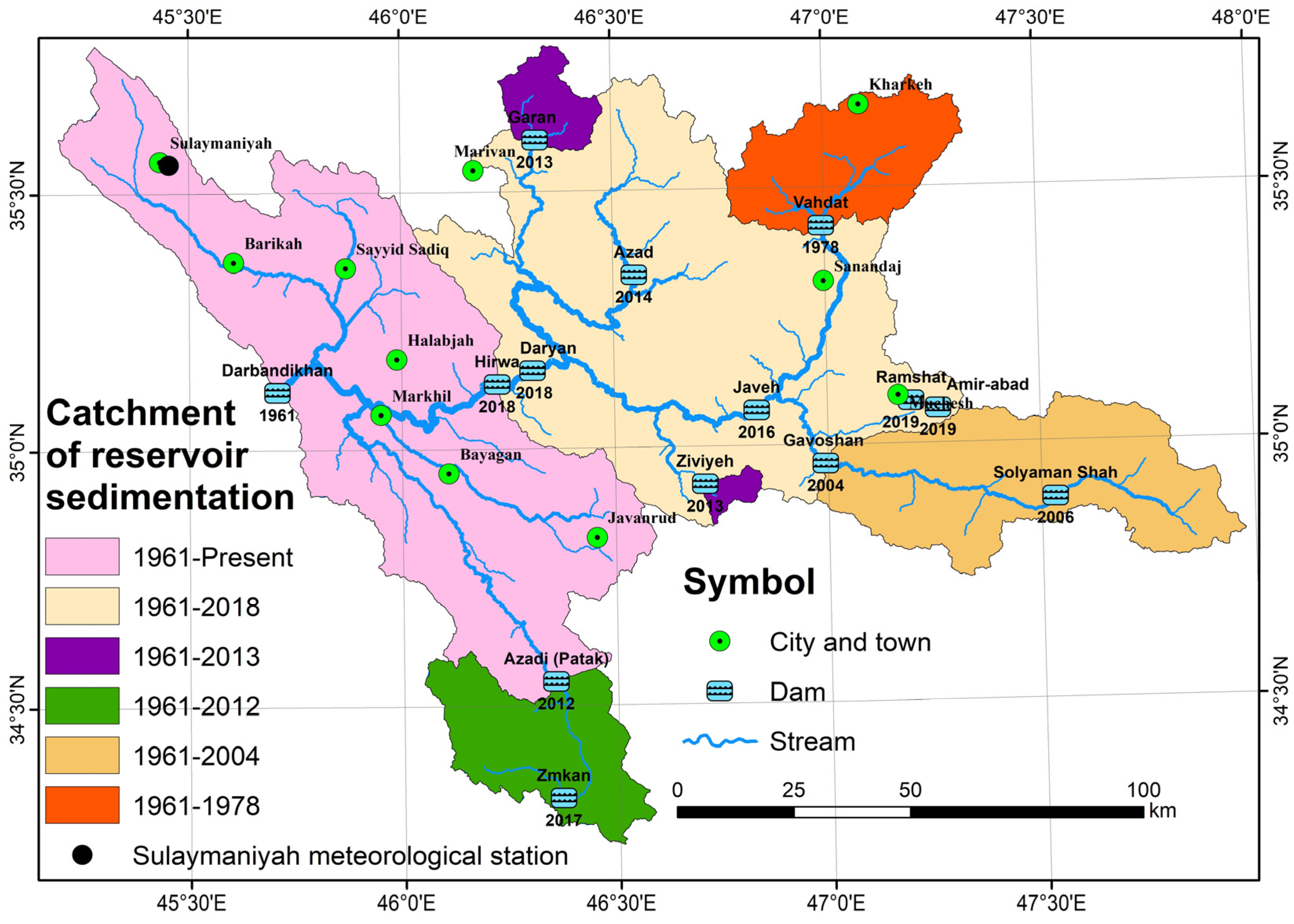
The Darbandikhan Lake Basin (DLB) is located in the northeastern part of Iraq/northwestern part of Iran between 45°11′20″E–47°58′43″E longitudes and 34°13′53″N–35°47′20″N latitudes (Figure 1). It covers a total area of 16,463.1 km2, and the major part is located in the northwestern part of Iran (13,155.28 km2, i.e., 79.91% of the total catchment area), while the minor part (3307.82 km2, i.e., 20.09% of the total catchment area) is located in Kurdistan Region, the northeastern part of Iraq (Figure 1).
The basin is located in a mountainous area, the elevation ranges from 450 m to 3351 m, and the major slope is directed towards the southwest of the area. The average annual precipitation for the last 20 years is 680 mm·y−1, with a major occurrence between October and April. The maximum temperature goes up to 45 °C in August, while the minimum temperature drops down to 3 °C in February [51].
The DL was formed after the construction of the Darbandikhan dam was completed, in November 1961 [52]. The DL feeds by the Sirwan (Diyala) River, which is a seventh-order river (according to the classification of [53]) and is located 55 km southeast of Sulaymaniyah city. The Sirwan River flows 270.4 km inside Iran before becoming part of the Iraq–Iran border for 43.1 km; then it flows 30.9 km inside Iraq until reaching the Darbandikhan dam, with a total length of 344.4 km. The maximum, minimum, and average annual discharge of the Sirwan river are 459.27 m3 s−1 (in 1969), 41.86 m3 s−1 (in 2000), and 153.26 m3 s−1 (1931–2004) [54].
From November 1961 to 1978, the dam’s catchment covers 16463.1 km2, which is also the sedimentation catchment of its reservoir (CRSed). In 1978, Iran built the first dam (Vahdat dam) within the catchment of the Darbandikhan dam [55]. Vahdat dam leads to a decrease in the CRSed to 15,403.5 km2. With the continuation of the dam construction (13 dams) within Iran, the water supply and the CRSed to DL decreased (Figure 2). The present situation shows that the CRSed for DLB is 5965.8 km2, representing 36.2% of the original catchment (Table 2).

3. Materials and Methods

3.1. Materials

Six scenes of the Digital Elevation Model (DEM) gathered by the Shuttle Radar Topography Mission (SRTM) were mosaicked [59]. The DEMs have a 30 m spatial resolution and are used to extract the drainage network, slope gradient, and flow accumulations. Due to the lack of in situ meteorological data, 3B43-V7 of the Tropical Rainfall Measuring Mission (TRMM) data [60] to construct a precipitation map were utilized. The monthly TRMM is with 0.25° × 0.25° spatial resolution [61]. The soil erodibility was determined by using the Harmonized World Soil Database (HWSD), which has a pixel size of ~852 m [62]. The AQUA eMODIS NDVI V6, with a spatial resolution of 250 m from 2003 to 2021, a scaling factor (of 10−4), and a radiometric resolution of 16-bit, was used to extract the C factor. The average of the C-factor value for the period from 2003 to 2021 has been used to cover the period from 2021 to 2002. The NDVI product can be accessed from the USGS webpage (https://earthexplorer.usgs.gov/ (accessed on 3 October 2022)) and is obtained by applying Equation (1), which is as follows:
N D V I = ρ N I R ρ R ρ N I R + ρ R
where ρ N I R and ρ R correspond to the surface reflectance of both the near-infrared (NIR) and red (R) wavebands of the MODIS, respectively.
Each NDVI scene covers 10-day composited datasets [63]; therefore, the approach suggested by Almagro et al. [64] was applied where four scenes per year were selected to cover the four seasons (i.e., 1–10 January, 1–10 April, 1–10 July, and 1–10 October). Such a strategy enabled us to capture of the variability of the natural vegetation.
Yearly global maps of MODIS land cover (MCD12Q1) were used, which was composed of a supervised classification (decision tree) algorithm of eight observation days by MODIS [65]. These data come with ~463 m spatial resolution, Nadir BRDF-Adjusted surface Reflectance [66], and land-surface temperature [67]. The data were downloaded from the main repository (https://lpdaac.usgs.gov/data, accessed on 3 October 2022) and covered the period from 2001 to 2020 with HDF file format, Sinusoidal grid, and multi-classification maps [65]. In this study, the International Geosphere-Biosphere Programme (IGBP) classification map was selected, encompassing 17 major land-cover classes in the scene. However, our study area includes only nine classes of land cover. All the data mentioned above are free of charge, and they were resized to 30 m cell size and reprojected to the Universal Transverse Mercator (UTM) projection/WGS 1984 datum within zone 38N, using the nearest neighbor resampling method to fit with the DEM scenes spatial resolution.
ArcGIS 10.8 software was used [68] to prepare the data, subset, and mosaic and perform the data operations, such as rater calculator, raster conversion, slope gradient, and stream flow accumulation. The connectivity index toolbox [69] was used to estimate the Index of Connectivity (IC). This toolbox works as a plugin within the ArcGIS environment. The drainage network and watershed boundaries were extracted by using TecDEM 2.2, a MATLAB-based toolbox [70]. Finally, r-based scripts were utilized to implement the statistical analysis [71].

3.2. Methods

Among all approaches, RUSLE has been widely used to estimate soil erosion under different conditions because it meets the need better than any other models available [2]. It has a huge number of works in the scientific literature and a large comparability of results, allowing researchers to adapt the model to nearly every type of condition and region of the world [2]. It is being used to predict long-period rates of rill and inter-rill erosion under different management practices around the globe [12,25]. It is a robust tool to estimate water erosion rates [72] and gives estimates on large spatial scales. Therefore, the RUSLE was chosen to estimate the SL in DL. Eighteen scenarios of RUSLE resulted from six R equations, and three models of the C factor, in addition to the LS, K, and P factors, were used to estimate the SL (Table A1 in Appendix A). The RUSLE was integrated with SDR (RUSLE-SDR) to estimate a 30 m spatial resolution of the RSed map for the DLB. RUSLE is widely employed [73] to assess the RSed, while the SDR is used to estimate the rate of erosion delivered to the lake. The model of Renard et al. [74] was used to calculate the RUSLE (Equation (2)).
A = R ·   K   ·   L S   ·   C   ·   P  
where A is the average annual rate of the soil loss (t·ha−1·y−1), R is the annual rainfall and runoff erosivity factor (MJ·mm·ha−1·h−1·y−1), K is the soil erodibility factor (t·ha·h·ha−1·MJ−1·mm−1), LS is the slope length and slope steepness factor, C is the cover management factor, and P is the support practice factor. The LS, C, and P factors are dimensionless. The following subsection describes the RUSLE’s factors.

3.2.1. Rainfall and Runoff Erosivity (R Factor)

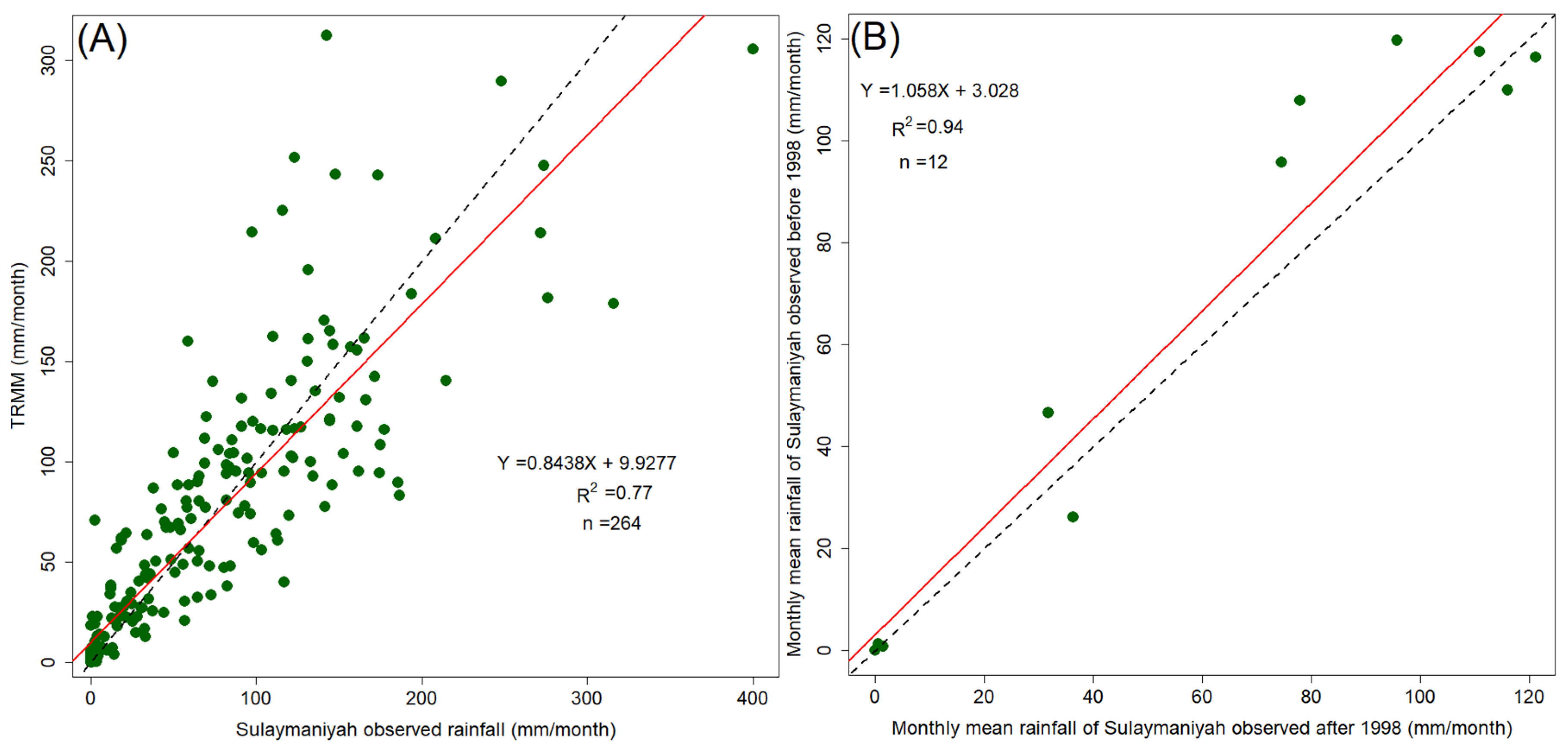
Erosion is caused by the driving force of rainfall [75]. The R factor represents the effect of precipitation impact on soil erosion [76]. The relationship between the R factor and precipitation have been determined in many regression analyses [31]. It requires precise and ongoing rainfall data [73]. The study area lacks climatic data records because it was a battlefield during the Iran–Iraq war; therefore, monthly TRMM (3B43–V7) data were used. The TRMM data are one of the main types of input data used to assess and compute the R factor [72,77]. For data validation, the TRMM data were compared with the observed metrological data and showed a good correlation with the observed metrological data (Figure 3). Moreover, TRMM data were proved by several researchers, such as [23,24,78,79,80], to be an applicable source of rainfall data for the Zagros region. However, the appropriateness of using TRMM data in the study area was evaluated by comparing 264 months of data with their corresponding data from the observed precipitation dataset from the Sulaymaniyah meteorological station (Figure 3A). This figure shows a strong direct relationship with a significant p-value < 0.05 and a coefficient of determination (R2) of 0.77. The comparison between monthly means of the 22 years (1998–2019) for the TRMM and Sulaymaniyah meteorological station shows a strong direct correlation with R2 of 0.94 (Figure 3B). The average annual precipitation of the DLB ranges between 352.78 mm·yr−1 (in the northeast) and 692.85 mm·yr−1 (in the northwest).
The TRMM pixels were vectorized in a points format, which was interpolated with a spatial resolution of 30 m, using the Inverse Distance Weighting (IDW) method. The pixel size was resampled to obtain the exact pixel size of the DEM. The resulting maps were used to estimate the R factor in six different models, which are Equation (3) [12,13,25], Equation (4) [13,23], Equation (5) [34,35,46,48,81], Equation (6) [29,82], Equation (7) [50,83], and Equation (8) [47,84,85].
The relationship between the R factor and precipitation alters widely based on the different climatic zones [31]. Therefore, the six equations (Table 3) were successfully tested in the Zagros countries (i.e., Iraq, Iran, and Turkey), which have similar climatic conditions to precisely select the R factor equation.
Where R is the runoff erosivity factor in MJ·mm·ha−1·h−1·y−1, P A is the average annual precipitation in mm, and MIF is the Modified Fournier index (Equation (9)), which was defined by Arnoldus [82]. The mean MIF was 80.79 mm, which is >55 mm.
M I F = I   =   1 12 P m 2 P A
where PA is the average annual precipitation (mm), Pm is the average monthly precipitation (mm), and R is the rainfall and runoff erosivity factor (MJ·mm·ha−1·h−1·y−1).

3.2.2. Soil Erodibility (K Factor)

The K factor expresses the potential soil vulnerability to erosion by the R factor [86]. In addition to soil texture, coarse fragments, structure, permeability, and organic matter play an effective role in the K factor value, where the increase in organic matter will decrease its susceptibility to separation [87].
The K factor was estimated by using Equations (10) and (11) [15,73]. The widely applied RUSLE was used to extract the K factor, and the HWSD dataset [88,89] was used to obtain soil texture and soil organic carbon information. Soil organic matter could be estimated from soil organic carbon using a conversion factor [90]. Based on the more reliable hypothesis that carbon represents 58% of the soil OM, the conversion factor will be 1.724 [90].
K = [ 2.1 × 10 4   M 1.14   ( 12 O M ) + 3.25 ( s 2 ) + 2.5 ( p 3 ) 100 ] 0.1317
M = ( m s i l t + m v f s ) ( 100 m c )
O M = 1.724 · O C
where mc is clay fraction content%; msilt silt fraction content%; mvfs very fine sand fraction content%; OM is the organic matter content%; OC is the soil organic carbon; and s is the soil structure class, and p is the permeability class, and they can be obtained in Table 4 and Table 5, respectively [15,73].

3.2.3. Slope Length (L Factor) and Slope Steepness (S Factor)

The slope-length factor reflects the impact of the terrain on the SL. Several equations have been suggested to estimate the L factor, such as [14,15,87]. Equations (13)–(15), suggested by Moore and Burch [91], were applied. Accordingly, the slope map (in percent) was extracted and classified into four groups, i.e., <1%, 1–3%, 3–5%, and ≥5%. Each group of the slope has its constant (m) (Equation (15)). Meanwhile, the S factor is calculated by using three slope (in percent) classes, which are <9%, 9–18%, and ≥18% (Equation (16); [92]).
L = ( λ 22.12848 ) m
λ = FA Ps
m = { 0.2                                                       θ < 1 % 0.3                               1 %   θ < 3 % 0.4                                 3 % θ < 5 % 0.5                                                       θ 5 %
S = { 10.8 · s i n θ + 0.03                                                       θ < 9 % 16.8 · s i n θ 0.05                         9 %   θ < 18 % 21.9 · s i n θ 0.96                                                     θ 18 %
where L is the slope length, S is the slope steepness factor, λ is the horizontal projection of slope length (m), m is a constant based on the value of slope gradient (Equation (15)), FA is stream flow accumulation, Ps is the pixel size of DEM, and θ is the slope gradient in percent.

3.2.4. Cover and Management (C Factor)

The C factor is the fraction of SL from an area with specific vegetation to the corresponding SL from a continuous fallow area [15]. It is one of the changeable erosion factors affected by human action [86]. In this study, three models, which have been used in the Zagros countries, were used to estimate the C factor. Equation (17) is the most common model [93], which has been tested in most of the articles surrounding the DLB, such as Iran [48,49], Turkey [27,33,94], and Iraq [23,26]. The second model to estimate the C factor used the land-cover maps. The land-cover model is applied in Turkey [28,29,31,32], Iran [25,46], and Iraq [25]. Nine land-cover classes of MCD12Q1 MODIS data exist in the DLB, which have different C-factor values (Table 6). The MCD12Q1 MODIS was used to estimate the C factor [77]. The third model was applied by using Equation (18) [95]. This model has been tested in Zagros countries, as well [35,44]. Equations (17) and (18) depend on MODIS NDVI to estimate the C factor, which has been widely applied [96,97,98,99,100].
C = E x p [ α · N D V I ( β N D V I ) ]
C = N D V I + 1 2
where α and β are constants, which are 2 and 1, respectively [101].

3.2.5. Support Practice (P Factor)

The P factor represents the fraction of the SL by an area with specific conservation soil to the corresponding loss upslope and downslope [14]. In DLB, Equation (19) was used. This equation was modified by Othman et al. [23] from the Wener Equation [103,104] to estimate the P factor.
P = 0.2 + 0.03 · θ
where P is the support practice factor, and θ is the slope angle in percent.

3.3. Sediment Delivery Ratio (SDR)

The SDR is the amount of the SL that actually reaches the specific outline at a specific time [6,20,105]. The range of the SDR is between 0 and 1 [106]. The SDR has been considered for a long time to be a constant number [21]; however, several models have been suggested to estimate the SDR. Most famous models are based on the nonlinear regression between the SDR and the basin area (Equation (20)) [105,107]. The area of the basin is the most affecting factor in determining the SDR for these models. This study considered the suggested models that were only used for estimating the SDR in basins that have an area close to that of DLB.
S D R = α · A b β
where the SDR is the sediment delivery ratio, the α and β are coefficients (Table 7), and the Ab is the basin area in km2.
Borselli et al. [22] suggested a new approach to estimating the SDR (SDR1; Equation (21)), which depends on calculating the IC (Equation (22)). The IC depends on the topographical information and can be calculated in an ArcGIS environment [22]. Topographic surface roughness (RI) was used to estimate the average weighting factor ( W ¯ ) (Equation (23)), which was suggested by [69]. The RI can be estimated by using Equation (24) [108].
Table 7. The α and β coefficients used to estimate the SDR in the DLB.
αβReferencesUnit of the AreaModel No.
0.47240.125[32,94,105]km2SDR2
1.8170.132[23,107]km2SRD3
2.9450.205[107]km2SDR4
0.510.11[77,109,110]mi2SDR5
S D R = S D R m a x 1 + e ( I C 0 I C i k b )
where SDR is the sediment delivery ratio; SDRmax is the maximum theoretical sediment delivery ratio, which is suggested to be 0.8 [6,21]; and IC0 and Kb are calibration parameters and equal to 0.5 and 2, respectively [12]. Both parameters can be determined by the S-shape of the sigmoid function relationship between the sediment delivery ratio and the IC [6]. The ICi is the index of connectivity for a specific cell.
I C = l o g 10 ( D u p D d n ) = l o g 10 ( W ¯ S ¯ A i d i W i S i )
where IC is the Index of Connectivity; Dup is the upslope components; Ddn is the downslope components; W ¯ is the average weighting factor of the contributing area; S ¯ is the average slope of the upslope contributing area (m/m); A is the area of the contribution (m2); and di, Wi, and Si, are the flow path to the main downstream channel, the weighting factor, and the slope gradient of the ith cell, respectively.
W i = 1 ( R I R I m a x )
R I = i   =   1 m w s 2 ( x i x ¯ ) 2 m w s 2
where Wi is the weighting factor, RI is the topographic surface roughness, mws is the moving window size (normally 5-cells; [108]), xi is the one specific cell value of the residual topography within the moving window, and x ¯ is the mean of the cells values within the moving window.

3.4. Reservoir Sedimentation (RSed)

Equation (25) [15] was used to estimate the RSed reached to DL in t·ha−1·yr−1. The absolute RSed for the six stages of the DLB areas were calculated in tons (Figure 2), where the DLB was changed with time as a result of the dams constructed within the basin (Table 2). Moreover, the amount of the RSed in tons was estimated until 2 May 2008, to validate the result of each scenario (see Section 4.2)
R S e d = R U S L E · S D R
where RSed is reservoir sedimentation, RUSLE is the soil loss, and SDR is the sediment delivery ratio.

3.5. Validation

For any model, validation is the most significant procedure to check the accuracy of the results [111]. The information about the RSed volume within the DL (Table A2 in Appendix B) offered by the ELC, Electroconsult; MED, Ingegneria; and SGI, Studio Galli Ingegneria companies [112] was used to validate the results of the 90 estimated scenarios of the RSed. Reference [112] used the historical topographic maps [113] produced before building the dam and a recent sub-water topographic map created by the topo-bathymetric survey by echo-sounding bathymetry data for the DL to estimate the amount of the RSed for the period between November 1961 and 2 May 2008.
The survey for the DL was implemented by [112] in clear, calm weather and water conditions. It was carried out between 25 April to 2 May 2008, at the dam sites, utilizing two small boats; an Echo sounder (Single beam Sonar Bathy500 Dual Frequency-200 kHz (10 degrees) Transducer) rod, and GPS (Positioning Trimble R6) antenna were mounted to the vessel via a wooden board manufactured directly at the site [112].
To convert the weight of the 90 scenarios (in tons) to size (in km3), three samples from the siltation within the DL were collected to find the average density of the siltation. Since the lake’s water level dropped as a result of the reduction in rainfall, the sediments exposed in the lake became a typical location to sample the actual sedimentation of the lake. The scenarios estimated the RSed in tons, while the siltation measured by the [112] is estimated in a million cubic meters (MCM).
All the results of the RUSLE factors, RUSLE, SDR, and RSed were presented for the periods between November 1961 to 2 May 2008. Finally, the RSed within the DL will be predicted by the end of 2019 using the best scenario out of the ninety scenarios tested. Moreover, the error rates were calculated using Equation (26):
E r r o r % = | ( i n   s i t u R S e d i n   s i t u ) · 100 |
where in situ means the results obtained by the surveys by echo-sounding bathymetry, and RSed is the outcome of the erosion model.
In addition, the only available survey for the DL, carried out between 25 April and 2 May 2008, is used indirectly to validate the estimation of the C and R factors, and the best scenario resulted from the best RUSLE and SDR combination for estimating the RSed.
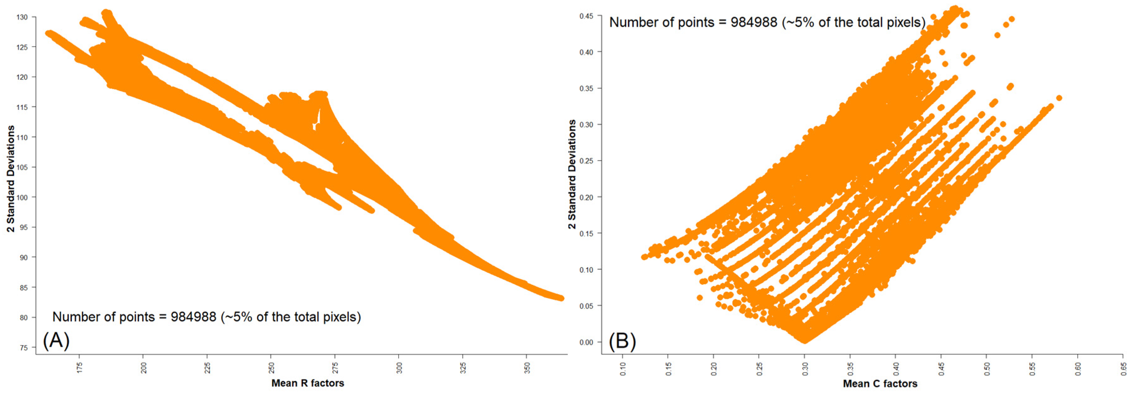
The error density plots display the relationship between the position and dispersion of the estimations for the factors (R and C). For this target, 984,988 pixels (~5% of the total pixels) were randomly selected and utilized. This test was repeated more than one time. The uncertainty plots display two standard deviations (SDs) of these estimates in the y-axis against their mean value in the x-axis, using the chosen pixels. The uncertainty plots allow the interpreter to determine the locations of the dispersion values for the estimated scenarios [80].

4. Results

The ninety scenarios of the RSed models for the DLB were estimated until 2 May 2008 and compared with the in situ surveys by echo-sounding bathymetry. The best RSed scenario resulting from this comparison was Scenario #18 (Table A2 in Appendix B). This scenario used Equation (5) to estimate the R factor, Equation (18) to estimate the C factor, and the IC model to estimate the SDR. Therefore, Equations (5) and (18) were reported to exhibit the result of the R factor and C factor, respectively, instead of other equations. In this section, a brief of all scenarios that were tested is given, and the focus will be on the optimum scenario result. The following subsections show the results of calculating RSed, SDR, RUSLE, and its factors.

4.1. Estimation RUSLE and Its Factors

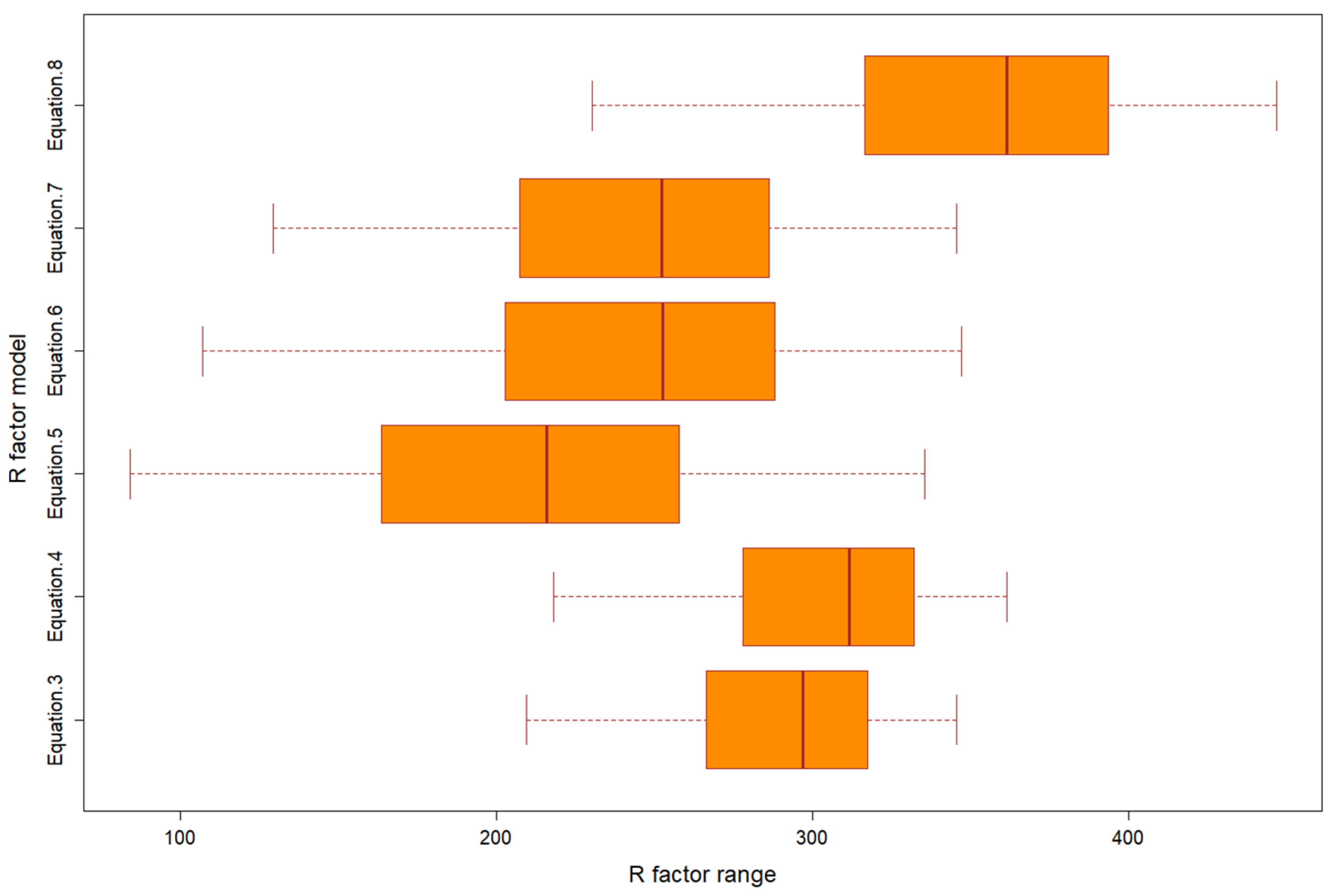
Table 8 shows six models of the R factor. The R factor resulting from Equation (5) varies from 83.69 MJ·mm·ha−1·h−1·y−1 to 335.47 MJ·mm·ha−1·h−1·y−1, with an average value of 210.4 MJ·mm·ha−1·h−1·y−1. The R-factor map was sliced into five classes, which decrease toward the east. The areas with very high class (>275 MJ·mm·ha−1·h−1·y−1) are located in the northwest, which is almost all located within Iraqi areas. Meanwhile, the regions with very low class are located in the eastern part of the DLB, within Iranian areas (Figure 4A). Figure 5 shows the distributions of the ~5% random selected pixels from R-factor values for the six equations. The R-factor distribution in Equation (8) has a higher performance than the others, while the performance of the R factors for Equations (5), (7), and (6) looks the same (Figure 5). Equations (3) and (4) have intermediate behavior between the two groups (i.e., Equations (5), (7), and (6); and Equations (3) and (4)).
Similarly, four types of soil were exposed in the study area. The majority of the DLB is loam texture, followed by clay and clay loam (Table 9). Figure 4B is the K-factor map, where the K factor value is low (0.023007 t·ha·h·ha−1·MJ−1·mm−1) in the northwestern part of the DLB, and the K factor value is high (0.063365 t·ha·h·ha−1·MJ−1·mm−1) in small patches in the north and northeastern parts of the DLB (Figure 4B).
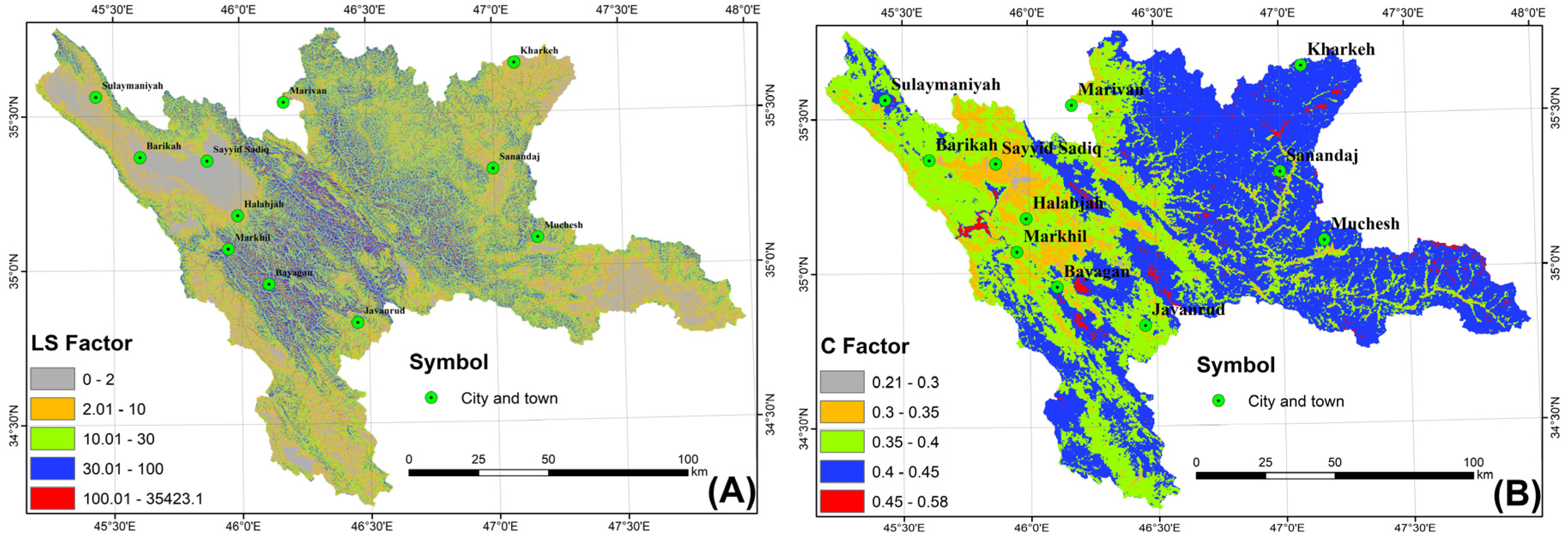
The slope gradient in the DLB reaches 77.6°, and the average is 16.2°. The majority of the high-slope areas are located in the central part of the DLB. This variation between the slopes, coupled with the variation in the flow accumulation, is the cause of the high fluctuation of the LS factor values. Likewise, the LS factor was sliced into five classes. Approximately 41.2% of the study area has LS < 1; almost all of these areas are located in the western part. The highest LS values (>100) cover 2.35% of the study area, while the average of the LS factor is 6.84 t·ha−1·y−1 (Figure 6A).
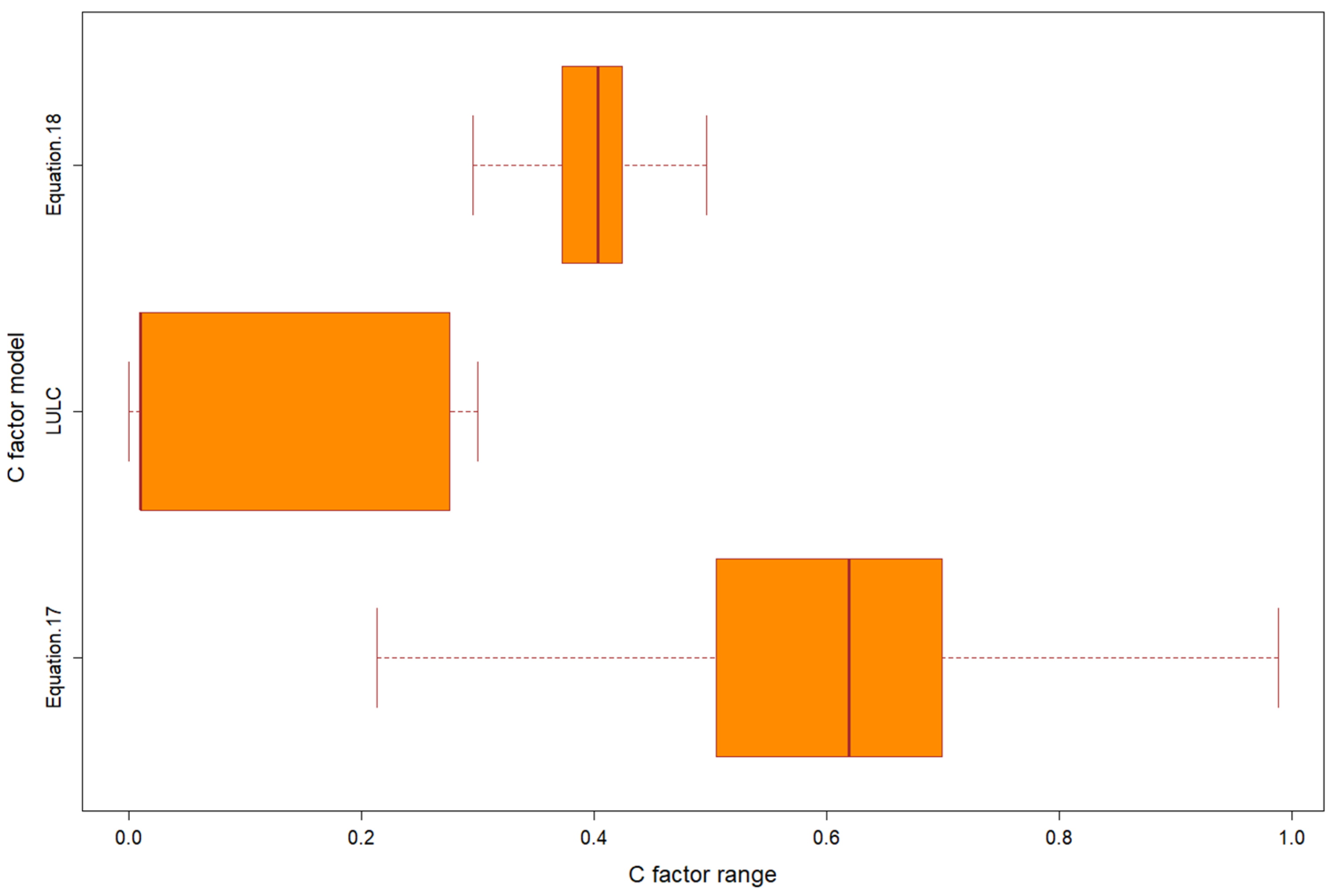
Similar to the R factor, the three calculated models of the C factor are stated in Table 10. The C factor ranged between 0.21 and 0.58 for Equation (18), which is classified into five classes (Figure 6B). The very high values (0.45–0.58) are located in the landslide and highly eroded areas (Figure 7A), which are distributed in small patches within the DLB. In general, the eastern part of the DLB has a C factor more than the western part (Figure 6B), while the lower values (<0.3) were presented in the forest and the agricultural areas (Figure 7B). Figure 8 shows the distributions of the ~5% random selected pixels from C-factor values for the three models (i.e., two equations and land-cover based), which have significant differences. The C-factor distribution in Equation (18) is higher than and the land-cover based one, while Equation (17) is higher than both (i.e., Equation (18) and land-cover based; Figure 8).
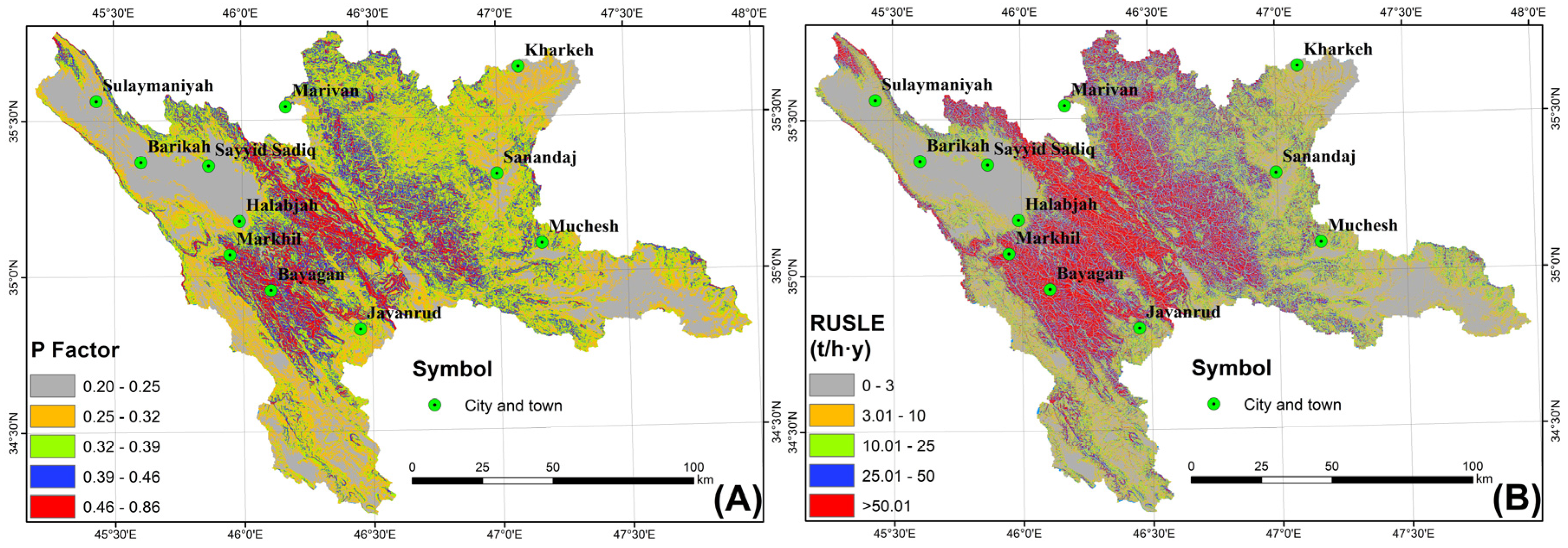
Similarly, Figure 9A shows the P factor, which is subdivided into five classes and ranges from 0.2 to 0.86. The very high P-factor values are located in the rough topography, which is mostly in the central part of the DLB. At the same time, the northwestern part of the study area shows low P-factor values.
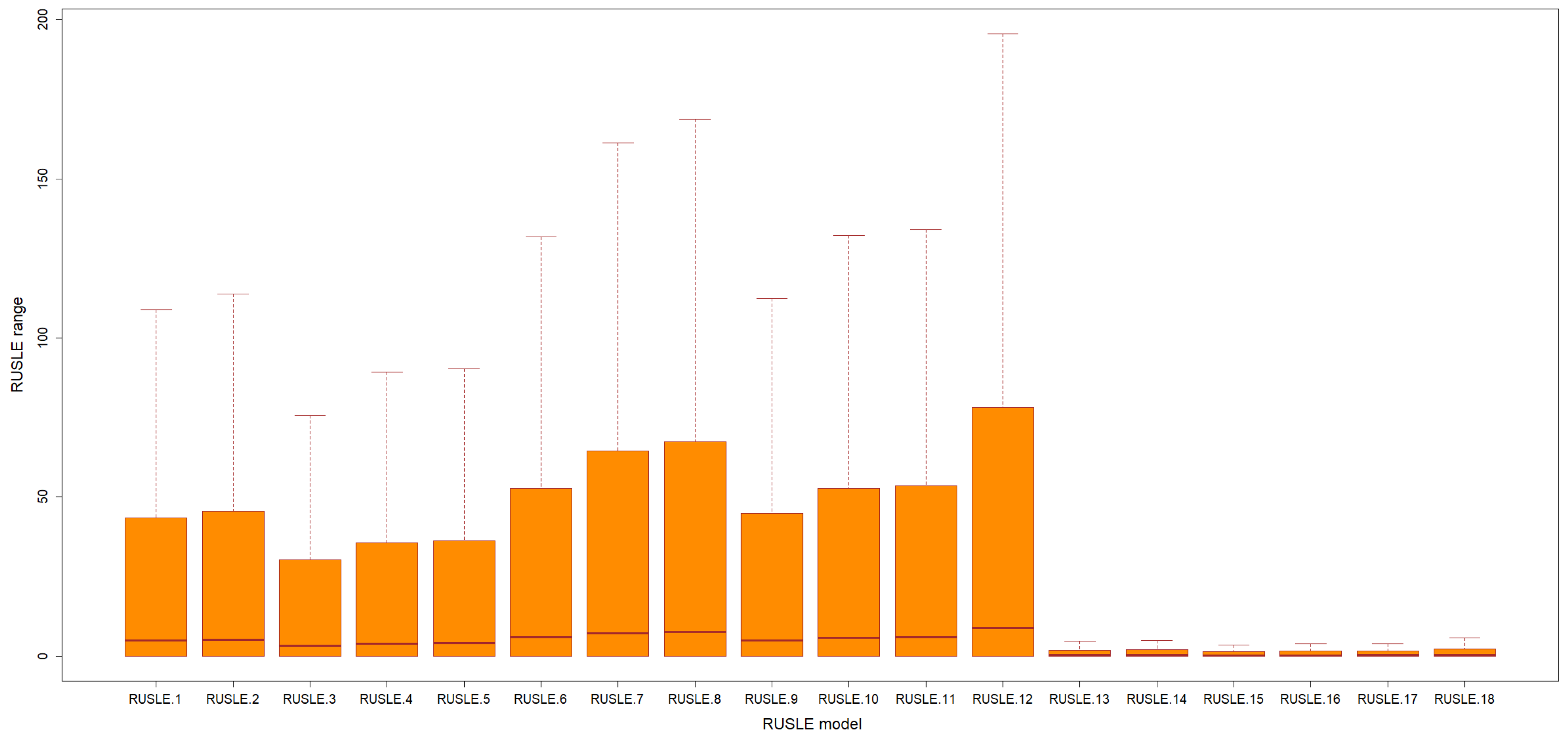
Figure 10 shows the distributions of one set of random selected pixels (~5% of the total data of the study area) from RUSLE model values for the eighteen scenarios, where more than one set was tested. More detailed information about the eighteen scenarios of RUSLE models of the R- and C-factor combinations can be found in Table A1 in Appendix A. It shows that there are two main groups (i.e., Group 1, RUSLE 1 to 12; and Group 2, RUSLE 13 to 18). The SL or RUSLE map was classified into five groups, ranging from 0 t·ha−1·y−1 to 83,628.8 t·ha−1·y−1, with an average value of 8.3 t·ha−1·y−1 (Figure 9B). The areas with very low and low SL (0–3 t·ha−1·y−1) represent >59% of the study area. They can be observed in the northwestern (near Sulaymaniyah city) parts of the DLB, in addition to the eastern parts (south of Muchesh and Sanandaj cities). Severe (12%) and very severe (15%) SL areas are located in the central part of the DLB. The extremely severe SL areas (>1000 t·ha−1·y−1) cover 0.15 of the DLB.

4.2. Sediment Delivery Ratio (DRr), Reservoir Sedimentation (RSed), and the Model Validation

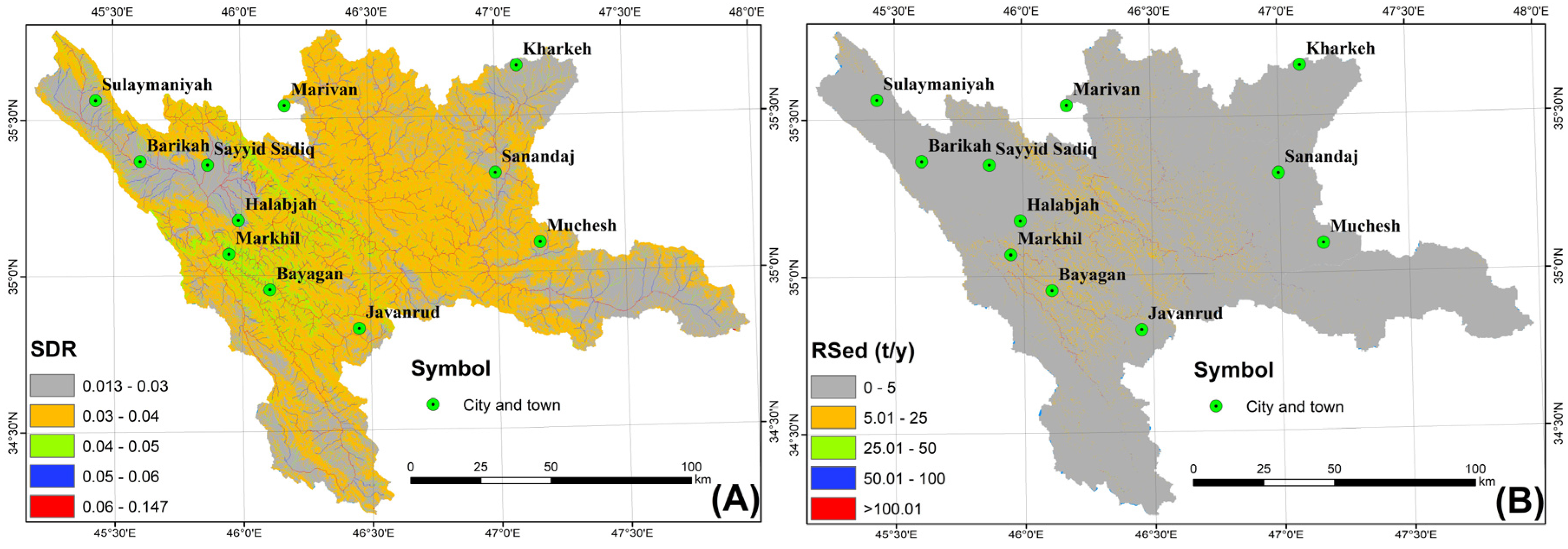
The five SDR models (i.e., the IC model and Table 7) show fluctuation in their results. Table 11 shows the statistical parameters of the SDR models. For the best scenario (IC model), the SDR ranges from 0.013 to 0.147, with an average value of 0.0327. The IC model map was classified into five classes (Figure 11A). The very high and high classes areas are located within and near the main valleys. In contrast, the very low and low classes areas can be observed in the northwestern (near Sulaymaniyah city) parts of the DLB, in addition to the eastern parts (south of Muchesh and Sanandaj cities).
The average density of the three samples collected from the field trip (1.631 kg/L) was used to convert the RSed scenarios from tons to km3. Figure 12 shows the distribution of part of the scenarios tested in this study (more than 20 km3·yr−1 and less than 50 km3·yr−1). The amount of Scenario #18, the best scenario (22.294 km3), makes it the closest model to the siltation measured by [112] within the DLB for the period from November 1961 to 2 May 2008, which is 22.223 km3. The average siltation per year is 0.46458 km3·yr−1. This scenario is followed by Scenarios #66, #61, and #62.
Almost all of the study areas are provided by the DLB with the sedimentation of <5 tons/year. Some of the areas, specifically in the central part of the DLB, provided the DLB with sedimentation between 5 and 50 tons/year. Very few areas (could be considered outliers) supplied the DLB with sedimentation >50 tons/year, which is normally located in the main streams (Figure 11B).

4.3. RUSLE, Its Factors, and Reservoir Sedimentation in the Present Day

The RUSLE for the DLB and the RSed within the DL were estimated by the end of 2019, using Scenario #18 (the best scenario out of the ninety scenarios tested). The RUSLE map was classified into five groups, ranging from 0 t·ha−1·y−1 to 82,725.2 t·ha−1·y−1, with an average value of 8.2 t·ha−1·y−1 (Figure 13A). The classes within the RUSLE maps show the same distribution for the old (2008) and new (2019) maps.
The average RSed within the DLB for the period from 2 May 2008 to 2 December 2019 is 0.3836 km3.yr−1 (Figure 13B). The total amount of the RSed within the DL for the period from November 1961 to the end of 2019 is 27.05 km3. The prediction of the RSed to the end of 2022 will be 28.201 km3.

5. Discussion

5.1. RUSLE-SDR and Its Factors

Two main insights must be considered when comparing predictions with in situ data. First, the model is valid to be applied to a specific area, which has its own circumstances. Therefore, almost all of the available Zagros literature was reviewed in the Scopus dataset [23,25,26,27,28,29,31,32,33,34,35,44,46,47,48,49,50,83,84,85,94]. Second, the successful prediction scenario must have an acceptable correlation with the in situ measurement. In this study, the final output of the 90 RSed scenarios was verified by using the bathymetry survey of the DL, which mirrors the verification of RUSLE factors and the SDR. When the bathymetry survey is compared with obtained RSed, Scenarios #18 and #66 give approximately similar results (the best; error < 1%), followed by Scenarios #61 and #62 (better; error < 10%), and then Scenarios #13 and #14 (good; error < 20%).
Among the six equations of the R factor, the equations that used MIF [82] give better results than other models, particularly Equations (5), (7), and (6), best, better, and good, respectively. Scenarios #18 and #66 used Equation (5) to estimate the R factor, while Scenarios #61 and #62 used Equations (7) and (6), respectively. Meanwhile Equation (8), which also depends on MIF, did not show a promising result (Table A3 in Appendix C, Table 12, and Figure 5). Moreover, the standard deviations of the R factor in the study area are lower than those of Azari et al. [47]. The results of the equations of the R factor are located within the range stated by Azari et al. [47]. Therefore, this study agrees with them to use the MIF models because of the impossibility of extracting the R factors in more suitable equations.
Scenario #18 used Equation (18), while Scenarios #66, #61, and #62 used the land-cover map to estimate the C factor. Scenario #18 used the IC model to estimate the SDR, while Scenarios #66, #61, and #62 used Equation (18), with α = 2.945 and β = 0.205 (Table A3 in Appendix C). This study shows that almost all (68 scenarios) of the prediction models are higher than the in situ measurement conducted by [112]. Eighteen scenarios are less than the in situ measurement.
This study recommends using SDR1 (IC) because it is changeable and can be applied for different area sizes and depends on the influence of topography on sediment connectivity [69], in contrast to SDR4, which depends on the area size and is affected by the change in landform. Moreover, the Zagros region is a mountainous area, varies in rock types and strengths, and has high tectonic activities [114], with medium to high erosional risk [115,116,117], confirming that this area suffers from severe erosion with low delivery for the soil. In addition, the results of RUSLE 3 correspond with the results of the research reported in the literature [25,31,32,45,48].
The scenarios of RSed, which have high accuracy, can be classified into two groups: scenarios with high SDR and low RUSLE and scenarios with low SDR and high RUSLE. The best SDRs are SDR1 and SDR4 because they comes three times for the best six scenarios (present of 50%), which has an accuracy >80 (Table 12). These two SDRs show variation in the delivery rate, as SDR1 ranges between 1.3% and 14.7%, while the mean SDR4 is 40.2%. Therefore, the SDR models can integrate these RUSLE models to obtain suitable results for the RSed, especially in inaccessible areas or areas with no verification. However, RUSLE 3 (includes C-factor Equation (18)) works better if it is coupled with SDR1 (Scenario #18), while RUSLE 15 (includes land-cover-based model) works better with SDR4 (Scenario #66; Table A3 in Appendix C and Table 12). In other words, the best combinations are represented by Scenario #18 (the best) and then Scenario #66 (better).

5.2. R Factor, C Factors, and RUSLE Uncertainties

Despite the variations and high uncertainty between the three models of the C factor, it appears that two models are valid in DLB: Equation (18) and land-cover models. Therefore, this study confirms that the selection of the C factor must consider the SDR model because of the high variation in the C-factor models (Figure 14B). This appears clearly in Figure 10, where the land-cover-based models (RUSLE 13-RUSLE18) have fewer distributions (low C-factor values) than the other RUSLE models. Moreover, increasing the number of NDVI scenes from one to three scenes per month will decrease the uncertainty of the C factor.
Table 12 emphasizes that the R factor does not play a big role in the discrepancy in the obtained results, especially for the six best scenarios of the RSed, where the same equation (i.e., Equation (5)) was used for Scenarios #18 and #66; Scenario #66 comes from land-cover-based models, and Scenario #18 comes from Equation (18). This is confirmed by Figure 14A, which displays that the variation between the six models is small, contrary to what appears in Figure 14B. However, the SDR models can be integrated with these RUSLE models to obtain suitable results for the RSed, especially in inaccessible areas or areas with no verification. Equation (18) works better if it is coupled with SDR1 (Scenario #18), while the land-cover model works better with SDR4 (Scenario #66; Table A3 in Appendix C and Table 12). In other words, the best combinations are represented by Scenario #18 (the best) and then Scenario #66 (better).
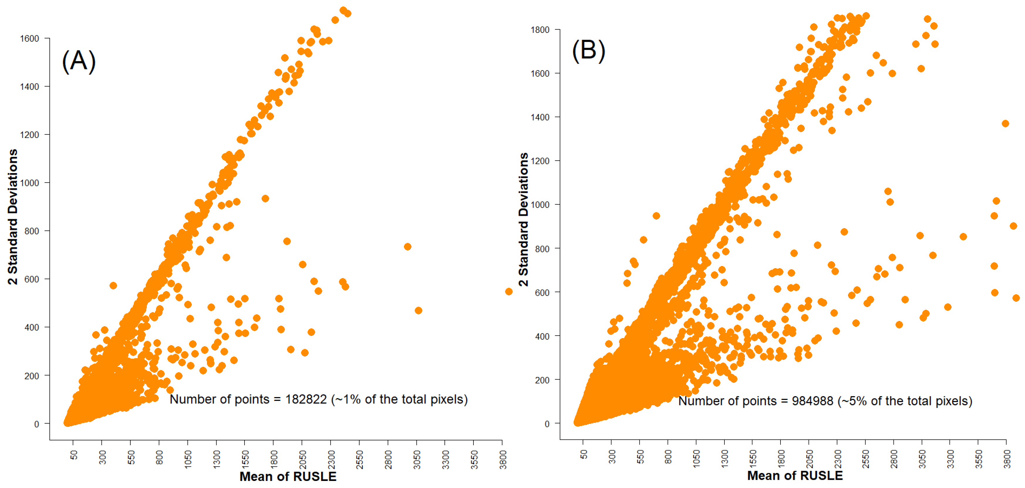
One of the variabilities of the results of the SRed is the uncertainty in the RUSLE models (Figure 15), which represents the distributions of the ~1% and ~5% randomly selected pixels from RUSLE model values for the eighteen scenarios. In both tests, i.e., Figure 15A,B, the pixels have low variation for the SL with high values, while the areas with low values have high variation. In other words, the uncertainty decreased with the SL values. The uncertainty of the RUSLE factors and SDR models is migrated to the RSed scenarios. The accuracy of the RUSLE factors and SDR models is significant; however, this requires field data for verification to evaluate these items [118], which requires carefully dealing with the local precipitation patterns and vegetation density [2], which is not an easy task [119].

5.3. Implications of This Study

Although 13 dams have been built within the DLB since 1978, the risk of RSed is present, as there was a decrease in the RSed amount from 0.46458 km3·yr−1 to 0.3836 km3·yr−1, i.e., 17.43% from the total amount. In comparison, the present catchment area for the DLB is decreasing to 36.2% of the original catchment (Table 1). It means that almost all of the areas (rugged Zagros mountains), which suffer from high and very high SL, are within the remaining catchments of the DL. Therefore, this study highly recommends keeping monitoring the RSed amounts in DLB and doing another bathymetry survey for this purpose. As a result, the new survey will emphasize our obtained findings, whose methodology can be applied and modified for other related and similar environments worldwide.

6. Conclusions

This study used the Revised Universal Soil Loss Equation (RUSLE)–Sediment Delivery Ratio (SDR) approach supported by multiple remote-sensing data sources to estimate the annual soil loss (SL) and reservoir sedimentation (RSed) in the Darbandikhan Lake Basin (DLB). For this purpose, eighteen RUSLE models coupled with five SDR models were used to estimate ninety scenarios of the RSed. The Digital Elevation Model (DEM), Tropical Rainfall Measuring Mission (TRMM), Harmonized World Soil Database (HWSD), and AQUA eMODIS NDVI V6 data were implemented for this end. The echo-sounding bathymetry survey was used to validate the results.
The research considered error factors, such as gravel and sand quarries, which may have a probable effect on decreasing the actual RSed. To check the scenario’s uncertainty, ~5% of the total pixels was used to investigate the relationship between the potion and the dispersion of the R and C factors estimation as a density plot.
The most proper model for the R and C factors and SDR was proposed in this research. Consequently, the most proper RUSLE-SDR model suitable for RSed modeling in the Zagros area was chosen based on the results from this research. Typical RUSLE (average of 8.3 t·ha−1·y−1) and RSed (average of 0.46458 km3·yr−1) for the Zagros region were proved by the results of this research. In addition, this research recommended avoiding the use of the Index of Connectivity (IC) model for calculating SDR and land cover for calculating the C Factor.
This study recommended using the Modified Fournier index (MIF) equations for estimating the R factor. It can be concluded that the scenarios of RSed, which have high accuracy, can be classified into two groups: scenarios with high SDR and low RUSLE and scenarios with low SDR and high RUSLE. For future work, we recommended increasing the number of scenes (three scenes per month) when calculating the C factor to reduce the uncertainty.

Author Contributions

Conceptualization, A.A.O. and S.S.A.; methodology, A.A.O. and S.S.A.; software, A.A.O.; validation, A.A.O. and S.G.S.; formal analysis, A.A.O.; investigation, A.A.O., S.S.A., S.G.S., A.K.O., O.A.-K. and V.L.; resources, A.A.O., S.S.A., S.G.S., A.K.O., O.A.-K. and V.L.; data curation, A.A.O.; writing—original draft preparation, A.A.O. and S.S.A.; writing—review and editing, A.A.O., S.S.A., S.G.S., A.K.O., O.A.-K. and V.L.; visualization, all authors; supervision, A.A.O. and S.S.A.; project administration, A.A.O. and S.S.A.; funding acquisition, S.S.A. and V.L. All authors have read and agreed to the published version of the manuscript.

Funding

This research received no external funding.

Data Availability Statement

Not applicable.

Acknowledgments

We thank USGS for providing Landsat and DEM data. We are grateful to the Darbandikhan Dam administration and Water Control Center in the Ministry of Water Resources, Iraq, for providing other useful data used in our study. We would like to thank the Food and Agriculture Organization (FAO) of the United Nations, the Chinese Academy of Sciences (CAS), the International Institute for Applied Systems Analysis (IIASA), the International Soil Reference and Information Centre (ISRIC), and Joint Research Centre of the European Commission (JRC) for supplying Harmonized world soil database (HWSD). We are grateful to the U.S. National Aeronautics and Space Administration (NASA) and the Japan Aerospace Exploration Agency (JAXA) for providing Tropical Rainfall Measuring Mission (TRMM) data. We also express our sincere gratitude to Hemin Ahmed Abdulla, geologist of the Darbandikhan Dam administration, for his assistance during the fieldwork and data collection. Ahmed Obaid acknowledges Salam Ismael Marhon for his encouragement and support. VL thanks CNPq, FAPESC, and UDESC. The fourth author thanks CARA for their great support to his academic research.

Conflicts of Interest

The authors declare no conflict of interest.

Appendix A

Table A1. The eighteen RUSLE scenarios of the R and C factors combinations were examined in Darbandikhan Lake for the period between November 1961 and 2 May 2022.
ScenariosC-EquationR-EquationScenariosC-EquationR-Equation
118310176
218411177
318512178
418613LC3
518714LC4
618815LC5
717316LC6
817417LC7
917518LC8

Appendix B

Table A2. The amount of the reservoir sedimentation gained for the period between November 1961 and 2 May 2008, within the Darbandikhan [112].
ElevationVOLUME DIFF (MCM)ElevationVOLUME DIFF (MCM)ElevationVOLUME DIFF (MCM)ElevationVOLUME DIFF (MCM)
434186.5196177449368.2601237464454.2837479444.557
435202.4116618450376.7507805465460.0191480454.4112
436217.8700461451383.6461686466462.8374481446.2946
437232.2080715452390.8162663467464.5166482434.6787
438246.3789168453397.2368461468465.7219483435.0195
439259.793523454402.6708382469467.6152484434.0626
440273.5651565455408.1217914470468.8454485423.8966
441285.4514375456412.3380251471469.2708486404.414
442297.1203966457416.9450171472469.4618487368.7144
443308.6056451458422.0896716473471.0426488323.7879
444319.7122029459427.3771193474472.0941489267.4594
445330.0812299460433.8615028475474.5954490209.1261
446340.4472993461438.4430503476471.8698491145.1009
447349.8499081462443.3719036477467.556649259.9097
448359.4951166463448.2591828478451.64464930

Appendix C

Table A3. The results of the scenarios examined in the Darbandikhan Lake for the period between November 1961 and 2 May 2022.
ScenariosC FactorR FactorSDRRSed (km3)Error%ScenariosC FactorR FactorSDRRSed (km3)Error %
1Equation (17)Equation (7)SDR136.9691666.355446Land coverEquation (3)SDR55.18185276.68248
2Equation (17)Equation (6)SDR137.0341866.6479847Land coverEquation (4)SDR55.41793575.62015
3Equation (17)Equation (8)SDR152.05412134.235348Land coverEquation (5)SDR54.16981681.23648
4Equation (17)Equation (3)SDR142.3881890.7401349Equation (18)Equation (7)SDR534.5785855.59816
5Equation (17)Equation (4)SDR147.80158115.099650Equation (18)Equation (6)SDR534.6359255.85619
6Equation (17)Equation (5)SDR132.4134345.8553351Equation (18)Equation (8)SDR548.8311119.7323
7Land coverEquation (7)SDR13.04592686.2938152Equation (18)Equation (3)SDR539.8827179.46591
8Land coverEquation (6)SDR13.06205386.2212453Equation (18)Equation (4)SDR541.7651287.93646
9Land coverEquation (8)SDR14.22134481.0046254Equation (18)Equation (5)SDR530.2086435.93412
10Land coverEquation (3)SDR13.41539384.6312755Equation (17)Equation (7)SDR4287.19741192.343
11Land coverEquation (4)SDR13.57505283.9128356Equation (17)Equation (6)SDR4287.06611191.752
12Land coverEquation (5)SDR12.71880587.7658157Equation (17)Equation (8)SDR4409.85231744.271
13Equation (18)Equation (7)SDR126.4984319.2387658Equation (17)Equation (3)SDR4336.91211416.051
14Equation (18)Equation (6)SDR126.5647719.5372859Equation (17)Equation (4)SDR4352.6921487.058
15Equation (18)Equation (8)SDR137.2021967.40460Equation (17)Equation (5)SDR4248.11581016.482
16Equation (18)Equation (3)SDR130.2406336.0780761Land coverEquation (7)SDR424.9661512.34374
17Equation (18)Equation (4)SDR131.6784142.5478662Land coverEquation (6)SDR425.0874112.88939
18Equation (18)Equation (5)SDR122.294160.32020963Land coverEquation (8)SDR434.4915855.20668
19Equation (17)Equation (7)SDR3358.53251513.3464Land coverEquation (3)SDR427.8948925.52261
20Equation (17)Equation (6)SDR3358.36811512.665Land coverEquation (4)SDR429.1657431.24124
21Equation (17)Equation (8)SDR3511.65612202.37266Land coverEquation (5)SDR422.446971.00783
22Equation (17)Equation (3)SDR3420.59861792.62767Equation (18)Equation (7)SDR4186.1391737.5966
23Equation (17)Equation (4)SDR3440.29781881.27168Equation (18)Equation (6)SDR4186.4481738.9871
24Equation (17)Equation (5)SDR3309.7421293.7969Equation (18)Equation (8)SDR4262.86011082.829
25Land coverEquation (7)SDR331.1666440.2449770Equation (18)Equation (3)SDR4214.6905866.0734
26Land coverEquation (6)SDR331.3180340.926271Equation (18)Equation (4)SDR4224.8236911.6708
27Land coverEquation (8)SDR343.0578793.7536372Equation (18)Equation (5)SDR4162.6163631.7477
28Land coverEquation (3)SDR334.8227856.6970373Equation (17)Equation (7)SDR299.73186348.7777
29Land coverEquation (4)SDR336.4092863.8360374Equation (17)Equation (6)SDR299.6861348.5717
30Land coverEquation (5)SDR328.0217726.0935575Equation (17)Equation (8)SDR2142.3258540.4437
31Equation (18)Equation (7)SDR3232.3718945.636576Equation (17)Equation (3)SDR2116.9967426.4667
32Equation (18)Equation (6)SDR3232.7572947.370777Equation (17)Equation (4)SDR2122.4763451.1241
33Equation (18)Equation (8)SDR3328.14991376.62378Equation (17)Equation (5)SDR286.1599287.706
34Equation (18)Equation (3)SDR3268.01581106.02979Land coverEquation (7)SDR28.66950660.98859
35Equation (18)Equation (4)SDR3280.66581162.95280Land coverEquation (6)SDR28.71161760.7991
36Equation (18)Equation (5)SDR3203.0056813.493281Land coverEquation (8)SDR211.9772546.10426
37Equation (17)Equation (7)SDR553.35229140.076982Land coverEquation (3)SDR29.68652156.41218
38Equation (17)Equation (6)SDR553.3278139.966783Land coverEquation (4)SDR210.1278354.42636
39Equation (17)Equation (8)SDR576.13834242.610584Land coverEquation (5)SDR27.79470964.92504
40Equation (17)Equation (3)SDR562.58831181.637585Equation (18)Equation (7)SDR264.63809190.8612
41Equation (17)Equation (4)SDR565.5197194.828386Equation (18)Equation (6)SDR264.74529191.3436
42Equation (17)Equation (5)SDR546.09182107.405987Equation (18)Equation (8)SDR291.28039310.7474
43Land coverEquation (7)SDR54.63779579.1306588Equation (18)Equation (3)SDR274.55308235.4771
44Land coverEquation (6)SDR54.66032379.0292889Equation (18)Equation (4)SDR278.07189251.3112
45Land coverEquation (8)SDR56.4072971.168290Equation (18)Equation (5)SDR256.46937154.1033

References

  1. Hajigholizadeh, M.; Melesse, A.M.; Fuentes, H.R. Erosion and Sediment Transport Modelling in Shallow Waters: A Review on Approaches, Models and Applications. Int. J. Environ. Res. Public Health 2018, 15, 518. [Google Scholar] [CrossRef] [PubMed] [Green Version]
  2. Alewell, C.; Borrelli, P.; Meusburger, K.; Panagos, P. Using the USLE: Chances, challenges and limitations of soil erosion modelling. Int. Soil Water Conserv. Res. 2019, 7, 203–225. [Google Scholar] [CrossRef]
  3. Kuznetsov, M.; Gendugov, V.; Khalilov, M.; Ivanuta, A. An equation of soil detachment by flow. Soil Tillage Res. 1998, 46, 97–102. [Google Scholar] [CrossRef]
  4. Pal, S. Identification of soil erosion vulnerable areas in Chandrabhaga river basin: A multi-criteria decision approach. Model. Earth Syst. Environ. 2016, 2, 5. [Google Scholar] [CrossRef] [Green Version]
  5. Walling, D.E. The Impact of Global Change on Erosion and Sediment Transport by Rivers: Current Progress and Future Challenges; UNESCO: London, UK, 2009. [Google Scholar]
  6. Hamel, P.; Chaplin-Kramer, R.; Sim, S.; Mueller, C. A new approach to modeling the sediment retention service (InVEST 3.0): Case study of the Cape Fear catchment, North Carolina, USA. Sci. Total. Environ. 2015, 524-525, 166–177. [Google Scholar] [CrossRef]
  7. Toy, T.J.; Foster, G.R.; Renard, K.G. Soil Erosion: Processes, Prediction, Measurement, and Control; Wiley: New York, NY, USA, 2002; ISBN 9780471383697. [Google Scholar]
  8. Montanarella, L.; Pennock, D.J.; McKenzie, N.; Badraoui, M.; Chude, V.; Baptista, I.; Mamo, T.; Yemefack, M.; Aulakh, M.S.; Yagi, K.; et al. World’s soils are under threat. Soild 2015, 2, 1263–1272. [Google Scholar] [CrossRef] [Green Version]
  9. Patro, E.R.; De Michele, C.; Granata, G.; Biagini, C. Assessment of current reservoir sedimentation rate and storage capacity loss: An Italian overview. J. Environ. Manag. 2022, 320, 115826. [Google Scholar] [CrossRef]
  10. World Commission on Dams. Dams and Development. A New Framework for Decision-Making. The Report of the World Commission on Dams; Earthscan: Oxford, UK, 2000. [Google Scholar]
  11. Cogollo, P.R.J.; Villela, S.M. Mathematical Model for Reservoir Silting. Sediment Budg. 1988, 174, 43–52. [Google Scholar]
  12. Rajbanshi, J.; Bhattacharya, S. Assessment of soil erosion, sediment yield and basin specific controlling factors using RUSLE-SDR and PLSR approach in Konar river basin, India. J. Hydrol. 2020, 587, 124935. [Google Scholar] [CrossRef]
  13. Majhi, A.; Shaw, R.; Mallick, K.; Patel, P.P. Towards improved USLE-based soil erosion modelling in India: A review of prevalent pitfalls and implementation of exemplar methods. Earth-Science Rev. 2021, 221, 103786. [Google Scholar] [CrossRef]
  14. Renard, K.G.; Foster, G.R.; Weesies, G.A.; McCool, D.K.; Yoder, D.C. Predicting Soil Erosion by Water: A Guide to Conservation Planning with the Revised Universal Soil Loss Equation (RUSLE); United States Department of Agriculture: Washington, DC, USA, 1997; Volume 703.
  15. Wischmeier, W.H.; Smith, D.D. Predicting Rainfall Erosion Losses: A Guide to Conservation Planning [USA]; Agriculture Handbook; United States Department of Agriculture: Washington, DC, USA, 1978.
  16. Brychta, J.; Podhrázská, J.; Šťastná, M. Review of methods of spatio-temporal evaluation of rainfall erosivity and their correct application. Catena 2022, 217, 106454. [Google Scholar] [CrossRef]
  17. Karan, S.K.; Ghosh, S.; Samadder, S.R. Identification of spatially distributed hotspots for soil loss and erosion potential in mining areas of Upper Damodar Basin—India. Catena 2019, 182, 104144. [Google Scholar] [CrossRef]
  18. Sonneveld, B.; Nearing, M. A nonparametric/parametric analysis of the Universal Soil Loss Equation. Catena 2003, 52, 9–21. [Google Scholar] [CrossRef] [Green Version]
  19. Cao, X.; Hu, X.; Han, M.; Jin, T.; Yang, X.; Yang, Y.; He, K.; Wang, Y.; Huang, J.; Xi, C.; et al. Characteristics and predictive models of hillslope erosion in burned areas in Xichang, China, on March 30, 2020. Catena 2022, 217, 106509. [Google Scholar] [CrossRef]
  20. Lu, H.; Moran, C.; Prosser, I.P. Modelling sediment delivery ratio over the Murray Darling Basin. Environ. Model. Softw. 2006, 21, 1297–1308. [Google Scholar] [CrossRef]
  21. Vigiak, O.; Borselli, L.; Newham, L.; McInnes, J.; Roberts, A. Comparison of conceptual landscape metrics to define hillslope-scale sediment delivery ratio. Geomorphology 2012, 138, 74–88. [Google Scholar] [CrossRef]
  22. Borselli, L.; Cassi, P.; Torri, D. Prolegomena to sediment and flow connectivity in the landscape: A GIS and field numerical assessment. Catena 2008, 75, 268–277. [Google Scholar] [CrossRef]
  23. Othman, A.A.; Obaid, A.K.; Al-Manmi, D.A.M.A.; Al-Maamar, A.F.; Hasan, S.E.; Liesenberg, V.; Shihab, A.T.; Al-Saady, Y.I. New Insight on Soil Loss Estimation in the Northwestern Region of the Zagros Fold and Thrust Belt. ISPRS Int. J. Geo-Inf. 2021, 10, 59. [Google Scholar] [CrossRef]
  24. Othman, A.A.; Obaid, A.K.; Sissakian, V.K.; Maamar, A.F.A.; Shihab, A.T. RUSLE Model in the Northwest Part of the Zagros Mountain Belt BT—Environmental Degradation in Asia: Land Degradation, Environmental Contamination, and Human Activities; Al-Quraishi, A.M.F., Mustafa, Y.T., Negm, A.M., Eds.; Springer International Publishing: Cham, Switzerland, 2022; pp. 287–306. ISBN 978-3-031-12112-8. [Google Scholar]
  25. Allafta, H.; Opp, C. Soil Erosion Assessment Using the RUSLE Model, Remote Sensing, and GIS in the Shatt Al-Arab Basin (Iraq-Iran). Appl. Sci. 2022, 12, 7776. [Google Scholar] [CrossRef]
  26. Al-Abadi, A.M.A.; Ghalib, H.B.; Al-Qurnawi, W.S. Estimation of Soil Erosion in Northern Kirkuk Governorate, Iraq Using Rusle, Remote Sensing and Gis. Carpathian J. Earth Environ. Sci. 2016, 11, 153–166. [Google Scholar]
  27. Bayazıt, Y.; Koç, C. The impact of forest fires on floods and erosion: Marmaris, Turkey. Environ. Dev. Sustain. 2022, 24, 13426–13445. [Google Scholar] [CrossRef]
  28. Imamoglu, A.; Dengiz, O. Determination of soil erosion risk using RUSLE model and soil organic carbon loss in Alaca catchment (Central Black Sea region, Turkey). Rend. Lincei 2017, 28, 11–23. [Google Scholar] [CrossRef]
  29. Ustaoğlu, B.; Ikiel, C.; Dutucu, A.A.; Koç, D.E. Erosion Susceptibility Analysis in Datça and Bozburun Peninsulas, Turkey. Iran. J. Sci. Technol. Trans. A Sci. 2021, 45, 557–570. [Google Scholar] [CrossRef]
  30. Sarp, G. Interaction between sediment transport rate and tectonic activity: The case of Kızılırmak Basin on the tectonically active NAFZ, Turkey. Arab. J. Geosci. 2020, 13, 265. [Google Scholar] [CrossRef]
  31. Irvem, A.; Topaloğlu, F.; Uygur, V. Estimating spatial distribution of soil loss over Seyhan River Basin in Turkey. J. Hydrol. 2007, 336, 30–37. [Google Scholar] [CrossRef]
  32. Ozsoy, G.; Aksoy, E.; Dirim, M.S.; Tumsavas, Z. Determination of Soil Erosion Risk in the Mustafakemalpasa River Basin, Turkey, Using the Revised Universal Soil Loss Equation, Geographic Information System, and Remote Sensing. Environ. Manag. 2012, 50, 679–694. [Google Scholar] [CrossRef]
  33. Ozsoy, G.; Aksoy, E. Estimation of soil erosion risk within an important agricultural sub-watershed in Bursa, Turkey, in relation to rapid urbanization. Environ. Monit. Assess. 2015, 187, 419. [Google Scholar] [CrossRef]
  34. Akbarzadeh, A.; Ghorbani-Dashtaki, S.; Naderi-Khorasgani, M.; Kerry, R.; Taghizadeh-Mehrjardi, R. Monitoring and assessment of soil erosion at micro-scale and macro-scale in forests affected by fire damage in northern Iran. Environ. Monit. Assess. 2016, 188, 699. [Google Scholar] [CrossRef]
  35. Arekhi, S.; Niazi, Y.; Kalteh, A.M. Soil erosion and sediment yield modeling using RS and GIS techniques: A case study, Iran. Arab. J. Geosci. 2012, 5, 285–296. [Google Scholar] [CrossRef]
  36. Fallah, M.; Kavian, A.; Omidvar, E. Watershed prioritization in order to implement soil and water conservation practices. Environ. Earth Sci. 2016, 75, 1248. [Google Scholar] [CrossRef]
  37. Vaezi, A.R.; Sadeghi, S.H.R. Evaluating the RUSLE model and developing an empirical equation for estimating soil erodibility factor in a semi-arid region. Span. J. Agric. Res. 2011, 9, 912. [Google Scholar] [CrossRef] [Green Version]
  38. Mirghaed, F.A.; Souri, B.; Mohammadzadeh, M.; Salmanmahiny, A.; Mirkarimi, S.H. Evaluation of the relationship between soil erosion and landscape metrics across Gorgan Watershed in northern Iran. Environ. Monit. Assess. 2018, 190, 643. [Google Scholar] [CrossRef]
  39. Mirakhorlo, M.S.; Rahimzadegan, M. Evaluating estimated sediment delivery by Revised Universal Soil Loss Equation (RUSLE) and Sediment Delivery Distributed (SEDD) in the Talar Watershed, Iran. Front. Earth Sci. 2020, 14, 50–62. [Google Scholar] [CrossRef]
  40. Zare, M.; Samani, A.A.N.; Mohammady, M.; Salmani, H.; Bazrafshan, J. Investigating effects of land use change scenarios on soil erosion using CLUE-s and RUSLE models. Int. J. Environ. Sci. Technol. 2017, 14, 1905–1918. [Google Scholar] [CrossRef]
  41. Zare, M.; Samani, A.A.N.; Mohammady, M.; Teimurian, T.; Bazrafshan, J. Simulation of soil erosion under the influence of climate change scenarios. Environ. Earth Sci. 2016, 75, 1405. [Google Scholar] [CrossRef]
  42. Ebrahimzadeh, S.; Motagh, M.; Mahboub, V.; Harijani, F.M. An improved RUSLE/SDR model for the evaluation of soil erosion. Environ. Earth Sci. 2018, 77, 454. [Google Scholar] [CrossRef]
  43. Avand, M.; Mohammadi, M.; Mirchooli, F.; Kavian, A.; Tiefenbacher, J.P. A New Approach for Smart Soil Erosion Modeling: Integration of Empirical and Machine-Learning Models. Environ. Model. Assess. 2022, 28, 145–160. [Google Scholar] [CrossRef]
  44. Damaneh, H.E.; Khosravi, H.; Habashi, K.; Tiefenbacher, J.P. The impact of land use and land cover changes on soil erosion in western Iran. Nat. Hazards 2022, 110, 2185–2205. [Google Scholar] [CrossRef]
  45. Zakeri, E.; Mousavi, S.A.; Karimzadeh, H. Scenario-based modelling of soil conservation function by rangeland vegetation cover in northeastern Iran. Environ. Earth Sci. 2020, 79, 107. [Google Scholar] [CrossRef]
  46. Mehri, A.; Salmanmahiny, A.; Tabrizi, A.R.M.; Mirkarimi, S.H.; Sadoddin, A. Investigation of likely effects of land use planning on reduction of soil erosion rate in river basins: Case study of the Gharesoo River Basin. Catena 2018, 167, 116–129. [Google Scholar] [CrossRef]
  47. Azari, M.; Oliaye, A.; Nearing, M.A. Expected climate change impacts on rainfall erosivity over Iran based on CMIP5 climate models. J. Hydrol. 2021, 593, 125826. [Google Scholar] [CrossRef]
  48. Derakhshan-Babaei, F.; Nosrati, K.; Mirghaed, F.A.; Egli, M. The interrelation between landform, land-use, erosion and soil quality in the Kan catchment of the Tehran province, central Iran. Catena 2021, 204, 105412. [Google Scholar] [CrossRef]
  49. Doulabian, S.; Toosi, A.S.; Calbimonte, G.H.; Tousi, E.G.; Alaghmand, S. Projected climate change impacts on soil erosion over Iran. J. Hydrol. 2021, 598, 126432. [Google Scholar] [CrossRef]
  50. Ostovari, Y.; Ghorbani-Dashtaki, S.; Kumar, L.; Shabani, F. Soil erodibility and its prediction in semi-arid regions. Arch. Agron. Soil Sci. 2019, 65, 1688–1703. [Google Scholar] [CrossRef]
  51. General Directorate of Research Agricultural Extension. Climate Data; Ministry of Agriculture of the Kurdistan Regional: Sulaimaniyah, Iraq, 2020. [Google Scholar]
  52. Yousif, O.S.Q.; Zaidn, K.; Alshkane, Y.; Khani, A.; Hama, S. Performance of Darbandikhan Dam during a Major Earthquake on November 12, 2017. In Proceedings of the EWG2019, 3rd Meeting of Dams and Earthquakes, An International Symposium, Lisbon, Portugal, 6–8 May 2019; pp. 295–308. [Google Scholar]
  53. Strahler, A.N. Quantitative analysis of watershed geomorphology. Eos Trans. Am. Geophys. Union 1957, 38, 913–920. [Google Scholar] [CrossRef] [Green Version]
  54. Saleh, D.K. Stream Gage Descriptions and Streamflow Statistics for Sites in the Tigris River and Euphrates River Basins, Iraq; U.S. Geological Survey: Reston, VA, USA, 2010. [Google Scholar] [CrossRef]
  55. Amini, A.; Bahrami, J.; Miraki, A. Effects of dam break on downstream dam and lands using GIS and Hec Ras: A decision basis for the safe operation of two successive dams. Int. J. River Basin Manag. 2021, 20, 487–498. [Google Scholar] [CrossRef]
  56. Rashidi, M.; Haeri, S.M. Evaluation of behaviors of earth and rockfill dams during construction and initial impounding using instrumentation data and numerical modeling. J. Rock Mech. Geotech. Eng. 2017, 9, 709–725. [Google Scholar] [CrossRef]
  57. Faraj, D.M.; Zaidan, K. The Impact of the Tropical Water Project on Darbandikhan Dam and Diyala River Basin. Iraqi J. Civ. Eng. 2022, 14, 1–6. [Google Scholar]
  58. Hosseini, S.P.; Jafari, R.; Esfahani, M.T.; Senn, J.; Hemami, M.-R.; Amiri, M. Investigating habitat degradation of Ursus arctos using species distribution modelling and remote sensing in Zagros Mountains of Iran. Arab. J. Geosci. 2021, 14, 2179. [Google Scholar] [CrossRef]
  59. Rabus, B.; Eineder, M.; Roth, A.; Bamler, R. The shuttle radar topography mission—A new class of digital elevation models acquired by spaceborne radar. ISPRS J. Photogramm. Remote Sens. 2003, 57, 241–262. [Google Scholar] [CrossRef]
  60. GSFC_DAAC. Tropical Rainfall Measurement Mission Project (TRMM; 3B43 V7). Available online: https://disc.gsfc.nasa.gov/datasets/TRMM_3B43_7/summary (accessed on 14 January 2023).
  61. Kummerow, C.; Barnes, W.; Kozu, T.; Shiue, J.; Simpson, J. The Tropical Rainfall Measuring Mission (TRMM) Sensor Package. J. Atmos. Ocean. Technol. 1998, 15, 809–817. [Google Scholar] [CrossRef]
  62. Nachtergaele, F.; van Velthuizen, H.; van Engelen, V.; Fischer, G.; Jones, A.; Montanarella, L.; Petri, M.; Prieler, S.; Teixeira, E.; Shi, X. Harmonized World Soil Database, version 1.2; FAO: Rome, Italy; IIASA: Laxenburg, Austria, 2012; pp. 1–50. [Google Scholar]
  63. Jenkerson, C.; Maiersperger, T.; Schmidt, G. EMODIS: A User-Friendly Data Source; U.S. Geological Survey: Reston, VA, USA, 2010.
  64. Almagro, A.; Thomé, T.C.; Colman, C.B.; Pereira, R.B.; Junior, J.M.; Rodrigues, D.B.B.; Oliveira, P.T.S. Improving cover and management factor (C-factor) estimation using remote sensing approaches for tropical regions. Int. Soil Water Conserv. Res. 2019, 7, 325–334. [Google Scholar] [CrossRef]
  65. NASA. User Guide for the MODIS Land Cover Type Product (MCD12Q1). 2013. Available online: https://lpdaac.usgs.gov/documents/438/MCD12Q1_User_Guide_V51.pdf (accessed on 14 January 2023).
  66. Wan, Z.; Zhang, Y.; Zhang, Q.; Li, Z.L. Validation of the land-surface temperature products retrieved from Terra Moderate Resolution Imaging Spectroradiometer data. Remote Sens. Environ. 2002, 83, 163–180. [Google Scholar] [CrossRef]
  67. Lina, H.; Wanga, J.; Jia, X.; Bo, Y.; Wang, D.; Wang, Z. Evaluation of Modis Land Cover Product of East China. In Proceedings of the International Geoscience and Remote Sensing Symposium (IGARSS), Boston, MA, USA, 8–11 July 2008; Volume 4, pp. IV762–IV765. [Google Scholar]
  68. ESRI. ArcGIS Desktop: Release 10.8; ESRI: Redlands, CA, USA, 2021. [Google Scholar]
  69. Cavalli, M.; Trevisani, S.; Comiti, F.; Marchi, L. Geomorphometric assessment of spatial sediment connectivity in small Alpine catchments. Geomorphology 2013, 188, 31–41. [Google Scholar] [CrossRef]
  70. Shahzad, F.; Gloaguen, R. TecDEM: A MATLAB based toolbox for tectonic geomorphology, Part 1: Drainage network preprocessing and stream profile analysis. Comput. Geosci. 2011, 37, 250–260. [Google Scholar] [CrossRef]
  71. R_Core_Team. R: A Language and Environment for Statistical Computing; R Foundation for Statistical Computing: Vienna, Austria, 2022. [Google Scholar]
  72. da Cunha, E.R.; Santos, C.A.G.; da Silva, R.M.; Panachuki, E.; de Oliveira, P.T.S.; Oliveira, N.D.S.; Falcão, K.D.S. Assessment of current and future land use/cover changes in soil erosion in the Rio da Prata basin (Brazil). Sci. Total. Environ. 2022, 818, 151811. [Google Scholar] [CrossRef]
  73. Panagos, P.; Meusburger, K.; Ballabio, C.; Borrelli, P.; Alewell, C. Soil erodibility in Europe: A high-resolution dataset based on LUCAS. Sci. Total Environ. 2014, 479–480, 189–200. [Google Scholar] [CrossRef]
  74. Renard, K.G.; Foster, G.R.; Weesies, G.A.; Porter, J.P. RUSLE: Revised Universal Soil Loss Equation. J. Soil Water Conserv. 1991, 46, 30–33. [Google Scholar]
  75. Sun, W.; Shao, Q.; Liu, J.; Zhai, J. Assessing the effects of land use and topography on soil erosion on the Loess Plateau in China. Catena 2014, 121, 151–163. [Google Scholar] [CrossRef]
  76. Kayet, N.; Pathak, K.; Chakrabarty, A.; Sahoo, S. Evaluation of soil loss estimation using the RUSLE model and SCS-CN method in hillslope mining areas. Int. Soil Water Conserv. Res. 2018, 6, 31–42. [Google Scholar] [CrossRef]
  77. Rosas, M.A.; Gutierrez, R.R. Assessing soil erosion risk at national scale in developing countries: The technical challenges, a proposed methodology, and a case history. Sci. Total. Environ. 2020, 703, 135474. [Google Scholar] [CrossRef] [PubMed]
  78. Salar, S.G.; Othman, A.A.; Rasooli, S.; Ali, S.S.; Al-Attar, Z.T.; Liesenberg, V. GIS-Based Modeling for Vegetated Land Fire Prediction in Qaradagh Area, Kurdistan Region, Iraq. Sustainability 2022, 14, 6194. [Google Scholar] [CrossRef]
  79. Othman, A.A.; Al-Maamar, A.F.; Al-Manmi, D.A.M.; Veraldo, L.; Hasan, S.E.; Obaid, A.K.; Al-Quraishi, A.M.F. GIS-Based Modeling for Selection of Dam Sites in the Kurdistan Region, Iraq. ISPRS Int. J. Geo-Inf. 2020, 9, 244. [Google Scholar] [CrossRef]
  80. Salar, S.G.; Othman, A.A.; Hasan, S.E. Identification of suitable sites for groundwater recharge in Awaspi watershed using GIS and remote sensing techniques. Environ. Earth Sci. 2018, 77, 701. [Google Scholar] [CrossRef]
  81. Renard, K.G.; Freimund, J.R. Using monthly precipitation data to estimate the R-factor in the revised USLE. J. Hydrol. 1994, 157, 287–306. [Google Scholar] [CrossRef]
  82. Arnoldus, H.M.J. An Approximation of the Rainfall Factor in the Universal Soil Loss Equation. In Assessment of Erosion; John Wiley and Sons: New York, NY, USA, 1980; pp. 127–132. [Google Scholar]
  83. Ostovari, Y.; Ghorbani-Dashtaki, S.; Bahrami, H.-A.; Naderi, M.; Dematte, J.A.M. Soil loss estimation using RUSLE model, GIS and remote sensing techniques: A case study from the Dembecha Watershed, Northwestern Ethiopia. Geoderma Reg. 2017, 11, 28–36. [Google Scholar] [CrossRef]
  84. Sadeghi, S.H.R.; Moatamednia, M.; Behzadfar, M. Spatial and Temporal Variations in the Rainfall Erosivity Factor in Iran TT. Journal of Agricultural Science and Technology 2011, 13, 451–464. [Google Scholar]
  85. Zabihi, M.; Sadeghi, S.H.; Vafakhah, M. Spatial Analysis of Rainfall Erosivity Index Patterns at Different Time Scales in Iran. Watershed Eng. Manag. 2015, 7, 442–457. [Google Scholar]
  86. Phinzi, K.; Ngetar, N.S. The assessment of water-borne erosion at catchment level using GIS-based RUSLE and remote sensing: A review. Int. Soil Water Conserv. Res. 2019, 7, 27–46. [Google Scholar] [CrossRef]
  87. Zerihun, M.; Mohammedyasin, M.S.; Sewnet, D.; Adem, A.A.; Lakew, M. Assessment of soil erosion using RUSLE, GIS and remote sensing in NW Ethiopia. Geoderma Reg. 2018, 12, 83–90. [Google Scholar] [CrossRef]
  88. Ijaz, M.A.; Ashraf, M.; Hamid, S.; Niaz, Y.; Waqas, M.M.; Tariq, M.A.U.R.; Saifullah, M.; Bhatti, M.T.; Tahir, A.A.; Ikram, K.; et al. Prediction of Sediment Yield in a Data-Scarce River Catchment at the Sub-Basin Scale Using Gridded Precipitation Datasets. Water 2022, 14, 1480. [Google Scholar] [CrossRef]
  89. Ali, M.G.; Ali, S.; Arshad, R.H.; Nazeer, A.; Waqas, M.M.; Waseem, M.; Aslam, R.A.; Cheema, M.J.M.; Leta, M.K.; Shauket, I. Estimation of Potential Soil Erosion and Sediment Yield: A Case Study of the Transboundary Chenab River Catchment. Water 2021, 13, 3647. [Google Scholar] [CrossRef]
  90. Kerven, G.L.; Menzies, N.; Geyer, M.D. Analytical methods and quality assurance. Commun. Soil Sci. Plant Anal. 2000, 31, 1935–1939. [Google Scholar] [CrossRef]
  91. Moore, I.D.; Burch, G.J. Physical Basis of the Length-slope Factor in the Universal Soil Loss Equation. Soil Sci. Soc. Am. J. 1986, 50, 1294–1298. [Google Scholar] [CrossRef]
  92. Li, Y.; Qi, S.; Liang, B.; Ma, J.; Cheng, B.; Ma, C.; Qiu, Y.; Chen, Q. Dangerous degree forecast of soil loss on highway slopes in mountainous areas of the Yunnan–Guizhou Plateau (China) using the Revised Universal Soil Loss Equation. Nat. Hazards Earth Syst. Sci. 2019, 19, 757–774. [Google Scholar] [CrossRef]
  93. Van der Knijff, J.M.; Jones, R.J.A.; Montanarella, L. Soil Erosion Risk: Assessment in Europe; European Commission: Brussels, Belgium, 2000. [Google Scholar]
  94. Ozsoy, G.; Aksoy, E. Prediction of soil loss differences and sediment accumulation at the Nilufer creek watershed, Turkey, using multiyear satellite data in a GIS. Geocarto Int. 2015, 30, 843–857. [Google Scholar] [CrossRef]
  95. Lin, C.-Y. A Study on the Width and Placement of Vegetated Buffer Strips in a Mudstone-Distributed Watershed. J. China Soil Water Conserv. 1997, 29, 250–266. [Google Scholar]
  96. Woznicki, S.A.; Cada, P.; Wickham, J.; Schmidt, M.; Baynes, J.; Mehaffey, M.; Neale, A. Sediment retention by natural landscapes in the conterminous United States. Sci. Total Environ. 2020, 745, 140972. [Google Scholar] [CrossRef]
  97. Xu, Z.; Zhang, S.; Zhou, Y.; Hou, X.; Yang, X. Characteristics of watershed dynamic sediment delivery based on improved RUSLE model. Catena 2022, 219, 106602. [Google Scholar] [CrossRef]
  98. Chuenchum, P.; Xu, M.; Tang, W. Estimation of Soil Erosion and Sediment Yield in the Lancang–Mekong River Using the Modified Revised Universal Soil Loss Equation and GIS Techniques. Water 2020, 12, 135. [Google Scholar] [CrossRef] [Green Version]
  99. Benavidez, R.; Jackson, B.; Maxwell, D.; Norton, K. A review of the (Revised) Universal Soil Loss Equation ((R)USLE): With a view to increasing its global applicability and improving soil loss estimates. Hydrol. Earth Syst. Sci. 2018, 22, 6059–6086. [Google Scholar] [CrossRef] [Green Version]
  100. Yigez, B.; Xiong, D.; Zhang, B.; Yuan, Y.; Baig, M.A.; Dahal, N.M.; Guadie, A.; Zhao, W.; Wu, Y. Spatial distribution of soil erosion and sediment yield in the Koshi River Basin, Nepal: A case study of Triyuga watershed. J. Soils Sediments 2021, 21, 3888–3905. [Google Scholar] [CrossRef]
  101. Durigon, V.L.; de Carvalho, D.F.; Antunes, M.A.H.; Oliveira, P.T.; Fernandes, M.M. NDVI time series for monitoring RUSLE cover management factor in a tropical watershed. Int. J. Remote Sens. 2014, 35, 441–453. [Google Scholar] [CrossRef]
  102. Bakker, M.M.; Govers, G.; van Doorn, A.; Quetier, F.; Chouvardas, D.; Rounsevell, M. The response of soil erosion and sediment export to land-use change in four areas of Europe: The importance of landscape pattern. Geomorphology 2008, 98, 213–226. [Google Scholar] [CrossRef]
  103. Terranova, O.; Antronico, L.; Coscarelli, R.; Iaquinta, P. Soil erosion risk scenarios in the Mediterranean environment using RUSLE and GIS: An application model for Calabria (southern Italy). Geomorphology 2009, 112, 228–245. [Google Scholar] [CrossRef]
  104. Fu, B.J.; Zhao, W.W.; Chen, L.D.; Zhang, Q.J.; Lü, Y.H.; Gulinck, H.; Poesen, J. Assessment of soil erosion at large watershed scale using RUSLE and GIS: A case study in the Loess Plateau of China. Land Degrad. Dev. 2005, 16, 73–85. [Google Scholar] [CrossRef]
  105. Vanoni Vito, A. Sedimentation Engineering, Manual and Reports on Engineering; Books; American Society of Civil Engineers: New York, NY, USA, 1975. [Google Scholar]
  106. Azizian, A.; Koohi, S. The effects of applying different DEM resolutions, DEM sources and flow tracing algorithms on LS factor and sediment yield estimation using USLE in Barajin river basin (BRB), Iran. Paddy Water Environ. 2021, 19, 453–468. [Google Scholar] [CrossRef]
  107. Sharda, V.N.; Ojasvi, P.R. A revised soil erosion budget for India: Role of reservoir sedimentation and land-use protection measures. Earth Surf. Process. Landf. 2016, 41, 2007–2023. [Google Scholar] [CrossRef]
  108. Cavalli, M.; Tarolli, P.; Marchi, L.; Fontana, G.D. The effectiveness of airborne LiDAR data in the recognition of channel-bed morphology. Catena 2008, 73, 249–260. [Google Scholar] [CrossRef]
  109. Ouyang, D.; Bartholic, J. Predicting Sediment Delivery Ratio in Saginaw Bay Watershed. In Proceedings of the 22nd National Association of Environmental Professionals Conference Orlando, Orlando, FL, USA, 19–23 May 1997. [Google Scholar]
  110. Behera, M.; Sena, D.R.; Mandal, U.; Kashyap, P.S.; Dash, S.S. Integrated GIS-based RUSLE approach for quantification of potential soil erosion under future climate change scenarios. Environ. Monit. Assess. 2020, 192, 733. [Google Scholar] [CrossRef]
  111. Chung, C.-J.F.; Fabbri, A.G. Validation of Spatial Prediction Models for Landslide Hazard Mapping. Nat. Hazards 2003, 30, 451–472. [Google Scholar] [CrossRef]
  112. ELC-Electroconsult; MED-Ingegneria; SGI—Studio Galli Ingegneria Dokan and Derbandikhan Emergency Hydropower Project, Final Reservoirs Topo-Bathymetric Report; Kurdistan Regional Government: Erbil, Iraq, 2009.
  113. General Authority of Survey Topographic Map Scale of 1:20000; Ministry of Water Resources, Water Control Center: Baghdad, Iraq, 1956.
  114. Othman, A.A.; Gloaguen, R.; Andreani, L.; Rahnama, M. Improving landslide susceptibility mapping using morphometric features in the Mawat area, Kurdistan Region, NE Iraq: Comparison of different statistical models. Geomorphology 2018, 319, 147–160. [Google Scholar] [CrossRef]
  115. CHRR; CIESIN; NGI. Global Landslide Hazard Distribution 2005; NASA Socioeconomic Data and Applications Center (SEDAC): Palisades, NY, USA, 2005. [Google Scholar]
  116. Othman, A.A.; Gloaguen, R. River Courses Affected by Landslides and Implications for Hazard Assessment: A High Resolution Remote Sensing Case Study in NE Iraq–W Iran. Remote Sens. 2013, 5, 1024–1044. [Google Scholar] [CrossRef] [Green Version]
  117. Othman, A.A.; Gloaguen, R. Automatic Extraction and Size Distribution of Landslides in Kurdistan Region, NE Iraq. Remote Sens. 2013, 5, 2389–2410. [Google Scholar] [CrossRef] [Green Version]
  118. Tanyaş, H.; Kolat, C.; Süzen, M.L. A new approach to estimate cover-management factor of RUSLE and validation of RUSLE model in the watershed of Kartalkaya Dam. J. Hydrol. 2015, 528, 584–598. [Google Scholar] [CrossRef]
  119. Wen, X.; Deng, X. Current soil erosion assessment in the Loess Plateau of China: A mini-review. J. Clean. Prod. 2020, 276, 123091. [Google Scholar] [CrossRef]
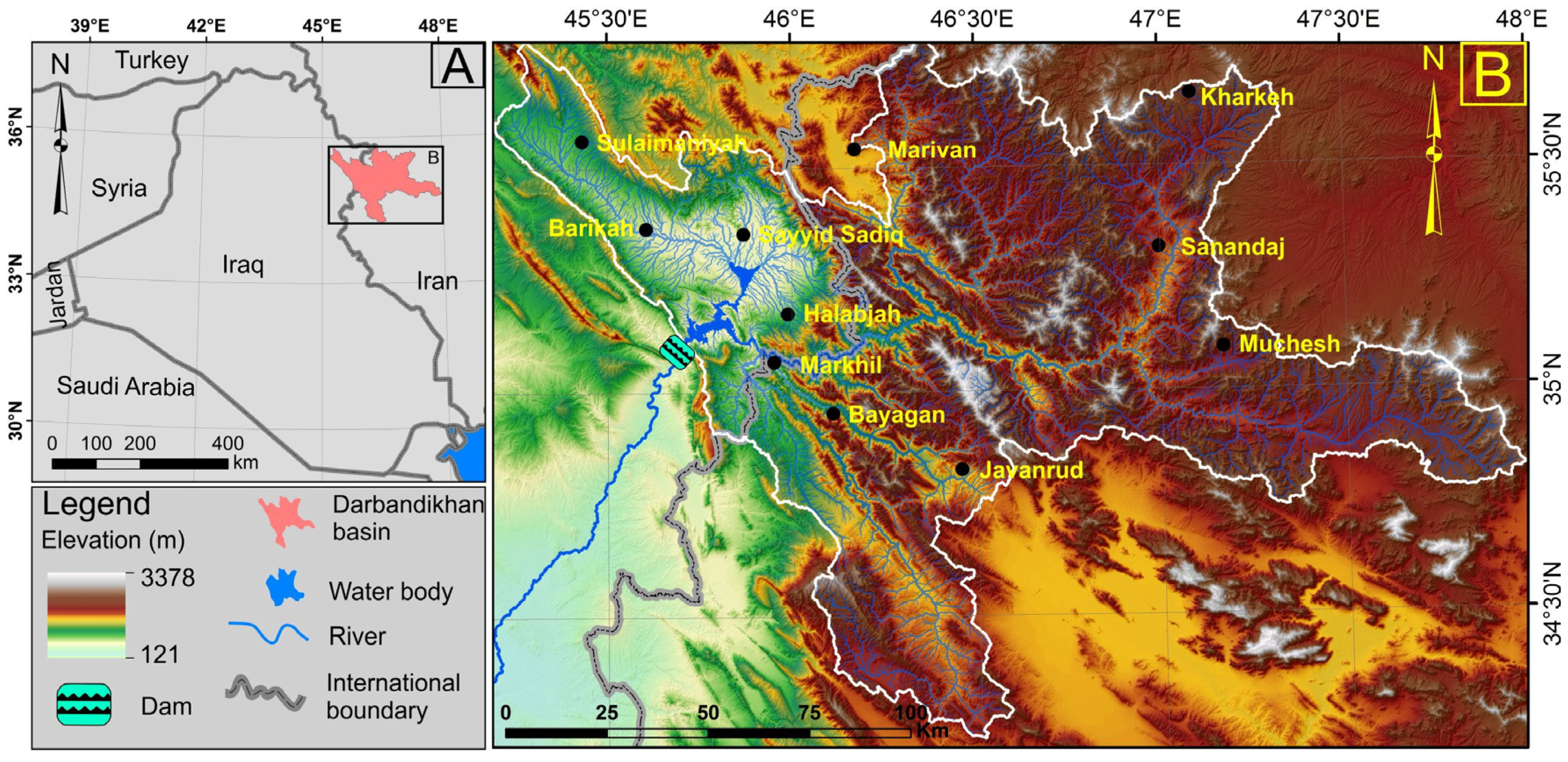
Figure 1. Location map of the Darbandikhan basin.
Remotesensing 15 00697 g001
Figure 2. Changing the area of the catchment area of the stream sediments for the Darbandikhan dam over time.
Remotesensing 15 00697 g002
Figure 3. Correlation between rainfall data collected at the Sulaymaniyah meteorological station and the corresponding cell of the TRMM data; (A) all months and (B) mean of the months of the year for the period between September 1998 and August 2019 [79].
Remotesensing 15 00697 g003
Figure 4. The distribution of the (A) R-factor (Equation (5)) and (B) K-factor maps within the DLB for 2 May 2008.
Remotesensing 15 00697 g004
Figure 5. Boxplot shows the distributions of the ~5% random selected pixels from R-factor values for the six equations used in this study, which is very rough.
Remotesensing 15 00697 g005
Figure 6. The distribution of the (A) LS factors and (B) C factors maps within the DLB for the period until 2 May 2008.
Remotesensing 15 00697 g006
Figure 7. The very high C-factor values were distributed in the (A) landslide (B) and agricultural areas overlayed by the QuickBird image (R3:G2:B1).
Remotesensing 15 00697 g007
Figure 8. Boxplot shows the distributions of the ~5% random selected pixels from C-factor values for the three equations used in this study.
Remotesensing 15 00697 g008
Figure 9. The distribution of the (A) P factors and (B) RUSLE maps within the DLB for the period until 2 May 2008.
Remotesensing 15 00697 g009
Figure 10. Boxplot shows the distributions of the ~5% random selected pixels from the 18 RUSLE scenarios used in this study (outlier pixels were removed).
Remotesensing 15 00697 g010
Figure 11. The distribution of the (A) sediment delivery ratio and (B) reservoir sedimentation maps within the DLB for the period until 2 May 2008.
Remotesensing 15 00697 g011
Figure 12. Evaluation of the reservoir sedimentation scenarios tested with the actual sedimentation in the Darbandikhan Lake Basin.
Remotesensing 15 00697 g012
Figure 13. The average distribution of the (A) RUSLE maps and (B) reservoir sedimentation maps within the DLB for the period until 2019.
Remotesensing 15 00697 g013
Figure 14. Uncertainty plots show the mean value of the factors estimates (x-axis) against two standard deviations of the factors estimates (y-axis) for (A) R factor and (B) C factor models.
Remotesensing 15 00697 g014
Figure 15. Uncertainty plots show the mean value of the eighteen RUSLE scenarios (x-axis) against two standard deviations of the eighteen RUSLE scenarios (y-axis); 124 outlier pixels of the RUSLE were removed, which are >5000 t·ha−1·y−1 for (A) ~1% and (B) ~5% of the total pixels was used.
Remotesensing 15 00697 g015
Table 1. List of acronyms and variables mentioned in the main text.
TermAbbreviationsTermAbbreviations
CCover managementPSupport practice parameter
CRSedSedimentation catchment of its reservoirRRainfall erosivity
DLDarbandikhan LakeRITopographic surface roughness
DLBDarbandikhan Lake BasinRSedReservoir Sedimentation
DEMDigital Elevation ModelRUSLERevised Universal Soil Loss Equation
HWSDHarmonized World Soil DatabaseSSlope steepness
ICIndex of ConnectivitySDStandard deviations
IDWInverse Distance WeightingSDRSediment Delivery Ratio
KSoil erodibilitySLSoil loss
LSlope lengthSRTMShuttle Radar Topography Mission
MCMMillion cubic metersTRMMTropical Rainfall Measuring Mission
MIFModified Fournier indexUSLEUniversal Soil Loss Equation
NDVINormalized Difference Vegetation IndexUTMUniversal Transverse Mercator
Table 2. Variation of the area of the Darbandikhan Dam catchment from 1961 to 2018.
PeriodArea of the Sedimentation Catchment for Darbandikhan Dam (km2)Area of the Catchment %Event and the YearReference of the Event
196116,463.1100Building Darbandikhan dam[52]
197815,403.593.6Building Vahdat dam[55]
200413,329.881.0Building Gavoshan dam[56]
201212,253.974.4Building Azadi dam[57]
201311,86572.1Building Garan and Ziviyeh dam[57]
20185965.836.2Building Hirwa and Daryan dams[58]
Table 3. Rainfall and runoff erosivity (R) factor models were tested in this study.
MethodThe Article Used within Iran–Iraq–TurkeyNoteEquation
R = 79 + 0.363   P A [25] (3)
R = 81.5 + 0.38   P A [23]340 < PA < 3500 mm(4)
R = 95.77 6.081 M I F + 0.447 M I F 2 17.2 [34,35,46,48]F > 55 mm(5)
R = ( 4.17 M I F ) 152 [29] (6)
R = 0.264 MIF 1.5 [50,83] (7)
R = 3.7628 M I F 3.532 [47,84,85] (8)
Table 4. Soil structure classes derived from the European Soil Database.
Structure Class (s)ValueSizeSoil Database
Very fine granular 11–2 mmG (good)
Fine granular22–5 mmN (normal)
Medium or coarse granular35–10 mmP (poor)
Blocky, platy, or massive4N10 mmH (peaty topsoil)
Table 5. Soil permeability classes are estimated from major soil textural classes.
Permeability ClassValueTexture
Fast and very fast1Sand
Moderate fast2Loamy sand, sandy loam
Moderate3Loam, silty loam
Moderate low4Sandy clay loam, clay loam
Slow5Silty clay loam, sand clay
Very slow6Silty clay, clay
Table 6. C factors weights for different land-cover classes in the DLB (Model 2).
NameC FactorReferences
Open Shrublands0.10[102]
Savannas0.05[102]
Grasslands0.01[102]
Permanent Wetlands0[13]
Croplands0.3[12,13,102]
Urban and Built-Up Lands0[13,102]
Cropland/Natural Vegetation Mosaics0.3[12,13,102]
Barren0[13,102]
Water Bodies0[12,13]
Table 8. R-factor parameters of the used models.
R FactorMinimumMaximumMeanSD
Equation (3)215.80332.54290.1425.44
Equation (4)224.71346.92302.5326.64
Equation (5)83.69335.47210.4064.18
Equation (6)106.75347.05242.7160.30
Equation (7)129.04345.63245.2854.81
Equation (8)229.95446.79352.6454.39
Table 9. Soil types, textures, and the K-factor values.
Soil TypeTexture ClassSand%Silt%Clay%K Factor
LithosolsLoam4334230.048767
Chromic VertisolsClay1629550.023007
Haplic XerosolsClay loam2333440.056780
Calcic XerosolsClay loam4037230.063365
Table 10. C-factor parameters of the used models.
C FactorMinimumMaximumMeanSD
Equation (17)0.02910. 6180. 13
Land cover00.30.0910.127
Equation (18)0.2130.5790. 3960. 034
Table 11. SDR ranges for the five models used in the DLB for the period between 1961 and 2008.
Model No.MinimumMaximumMeanSD
10.1250.1280.1260.0014
20.5090.5190.5110.0059
30.4020.4200.4100.0074
40.1720.1760.1740.0017
IC (Equation (22))0.0130. 1470.03270.0076
Table 12. The results of the best scenarios, which have error rates less than 20% in the Darbandikhan Lake for the period between November 1961 and May 02, 2022.
ScenariosC FactorR FactorSDRRSed (km3)Error %
18Equation (18)Equation (5)SDR122.290.32
66Land coverEquation (5)SDR422.4451.01
61Land coverEquation (7)SDR424.9712.34
62Land coverEquation (6)SDR425.0912.89
13Equation (18)Equation (7)SDR126.5019.24
14Equation (18)Equation (6)SDR126.5719.54
Disclaimer/Publisher’s Note: The statements, opinions and data contained in all publications are solely those of the individual author(s) and contributor(s) and not of MDPI and/or the editor(s). MDPI and/or the editor(s) disclaim responsibility for any injury to people or property resulting from any ideas, methods, instructions or products referred to in the content.