Fast Wideband Beamforming Using Convolutional Neural Network

Abstract

With the wideband beamforming approaches, the synthetic aperture radar (SAR) could achieve high azimuth resolution and wide swath. However, the performance of conventional adaptive wideband time-domain beamforming is severely affected as the received signal snapshots are insufficient for adaptive approaches. In this paper, a wideband beamformer using convolutional neural network (CNN) method, namely, frequency constraint wideband beamforming prediction network (WBPNet), is proposed to obtain a satisfactory performance in the circumstances of scanty snapshots. The proposed WBPNet successfully estimates the direction of arrival of interference with scanty snapshots and obtains the optimal weights with effectively null for the interference by utilizing the uniqueness of CNN to extract potential nonlinear features of input information. Meanwhile, the novel beamformer has an undistorted response to the wideband signal of interest. Compared with the conventional time-domain wideband beamforming algorithm, the proposed method can fast obtain adaptive weights because of using few snapshots. Moreover, the proposed WBPNet has a satisfactory performance on wideband beamforming with low computational complexity because it avoids the inverse operation of covariance matrix. Simulation results show the meliority and feasibility of the proposed approach.

1. Introduction

Radio Frequency Interference (RFI) is a growing problem in Synthetic Aperture Radar (SAR) systems. The advanced SAR radars with Digital Beamforming (DBF) are capable of notching the antenna pattern in specific directions, which can be utilized to suppress RFI on board or in post-processing [1]. Meanwhile, to address the problem of reduced echo gain and insufficient interference suppression, the adaptive beamforming has been proposed. However, the process of adaptive beamforming is extremely computationally demanding because of the need for processing range bin by range bin, limiting the possibility of real-time processing on the future spaceborne space-time waveform encoding (STWE) SAR in elevation [2]. As is concluded in [3,4], using wideband DBF on the receive array can overcome the dilemma of a trade-off between high azimuth resolution and wide swath in SAR [5]. Since SAR uses wideband waveforms to obtain range and azimuth resolution meanwhile high-resolution inverse SAR (ISAR) imaging requires transmission of wideband signal [6,7], research on adaptive wideband DBF is very important for SAR. At present, the main beamforming method is to alter the element weight coefficients with the change of wideband frequency, which can be implemented in frequency-domain and time-domain respectively. The wideband frequency-domain beamforming, which primarily adopts discrete Fourier transformation (DFT) and inverse discrete Fourier transformation (IDFT), is a subband division and processing method based on narrowband signal superposition [8]. The wideband time-domain beamforming is realized by amplitude weighting, time delay and sum of each array element. One of the most classic structures is the Frost [9] beamformer (FB), where the data of array elements are processed via tapping-delay-lines (TDLs) and addressed with the linear constrained minimum variance (LCMV) criterion. The FB needs adjusting delay structures to keep steering to the wideband signal of interest (SOI). However, the practical application of pre-steering delays in the analog or digital domain may cause insurmountability errors of time delay [10]. Then, using frequency constraints to exclude delay structures is proposed for the FB in [11].

Deep learning (DL) uses deep neural networks (NNs) as function approximators and it is more robust to deal with different targets imaging [12], the application of NNs have penetrated into almost all engineering fields and set off a new wave of research with its particular advantages, especially in image classification, speech recognition and task regression [13]. Thereinto, the main goal of a regression task is to predict continuous (numerical) variables, whereas classification is used for the prediction of discrete (categorical) variables [14]. Moreover, during the past decades, combining NN with beamforming technology to improve performance is a popular trend. Considering the complex inter-frequency interactions, leading to sub-optimal filter characteristics and non-uniform beamwidth, a beamforming NN architecture is proposed in [15] to obtain a uniform beamwidth. However, the discussion in [15] only focus on the narrowband signal model in the frequency domain.

The convolutional NN (CNN), with its sufficient model capacity and sparse connectivity, could reconstruct complex models and learn nonlinear function relations from abundant training data to further implement generalization [16,17]. Moreover, the weight parameters contained in CNN are shared with each other, leading to less number of parameters. Therefore, CNN is employed to improve efficiency in relevant research, such as text detection [18] and image quality enhancement [19]. In recent years, the CNN has developed rapidly, and it have gained extensive attention and great success in the field of beamforming [20]. A CNN structure, which is trained with inputs/outputs (I/O) pairs to compute the optimum Wiener solution, is presented in [21]. In addition, the structure obtains the robust and fast beamforming of phased array antenna without high computational complexity. Then, a neural beamformer is presented in [22] to estimate the SOI. It employs a CNN to suppress interferences and a long short-term memory (LSTM) to estimate the SOIs. Compared with the conventional beamformers such as the minimum variance distortionless response (MVDR), the proposed neural beamformer achieves higher output signal to interference plus noise ratio (SINR) than the conventional MVDR with mismatches of estimated autocorrelation matrix. Besides, [23] proposes a method to employ the CNN for evaluating the desired signals in the presence of narrowband and wideband interferences. In [24], a fast and robust adaptive beamforming method based on complex-valued radial basis function (CRBF) neural network is proposed to prevent the matrix inversion operation in the existing adaptive beamforming methods, which results in large amounts of computational complexity. Due to the significant importance of beamforming design for large scale antenna arrays in millimeter wave communication systems, a beamforming NN is trained in [25]. The proposed beamforming NN in [25] successfully learns how to optimize the beamformer for maximizing the spectral efficiency with hardware limitation and imperfect channel state information. Using 4 convolutional layers and 4 fully-connected layers in [26], the CNN processes a desired two dimensional radiation pattern and calculates the phase values for array beamforming. Dual cost functions are alternatively used in [27] during the training process, this method can solve the contradiction between nonlinear beamformers and the annoying distortion on the output target signals.

To solve the problem that the time-domain wideband beamformers fail to obtain appropriate weights when the snapshots is insufficient, we propose an approach to implement adaptive time-domain frequency constraint Frost beamformer (FCFB) structure on the basis of CNN, namely wideband beamforming prediction network (WBPNet). The unit in the convolutional layers (CONV layers) of CNN connections is restricted to only a few regions of the input data. By sharing the connection parameters between different units, the novel model can extract the same pattern, regardless of its position at the entrance. Such a configuration gives rise to layers capable of extracting elementary characteristics, which can be combined into deeper layers to obtain complex data representations [28]. The whole WBPNet can be divided into offline training stage and online performance stage. The training samples in the offline stage are the received vectors under the condition of few snapshots, sharply reducing the computation complexity for the prevention of autocorrelation matrix. Then, to maximally retain the inherent relation of the real and imaginary parts of training data, inputs are transferred to a dual-channel model. What needs illustration is that our training samples contain certain range in directions of arrival (DOAs) of interference, indicating that the proposed network has adequate universal relevance on the DOAs of interference in the online cases. Finally, the trained network successfully obtains the optimum weights, avoids the huge amount of computation required by the analytical solutions, and improves the inflexibility of iterative solutions.

The rest of this paper is organized as follows. Section 2 expounds the wideband signal model briefly. In Section 3, the proposed method based on CNN is explained in detail. Section 4 demonstrates the simulation comparison results and gives the related analyses. Ultimately, Section 5 provides the conclusion.

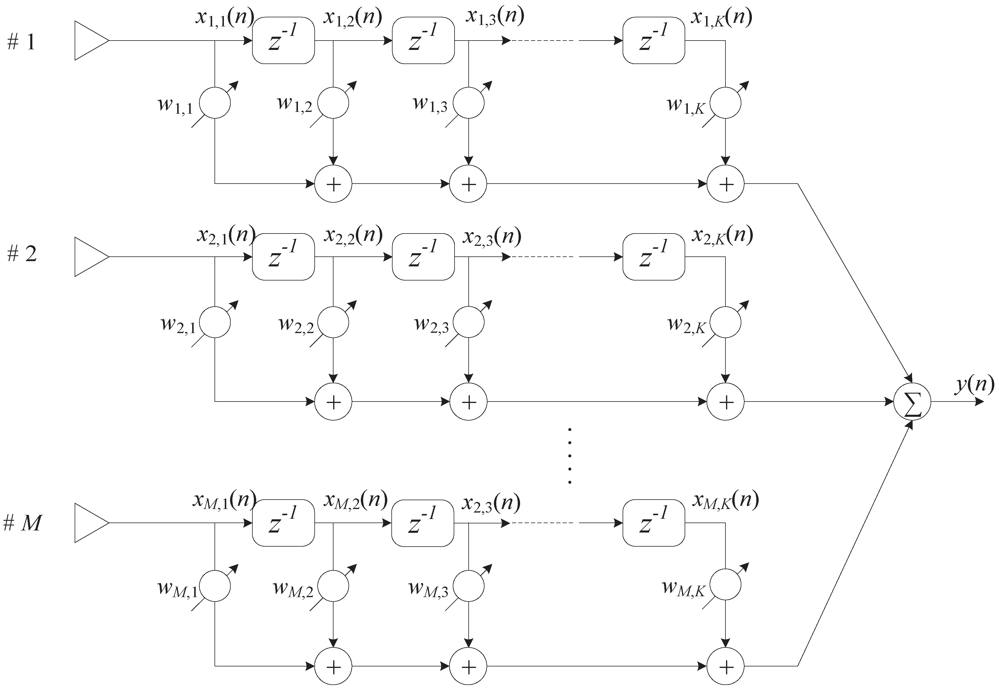
2. Wideband Signal Model

The conventional structure in time-domain wideband beamforming technologies, requires delay structures to achieve an undistorted response to SOI [9]. The delay structures cause some errors in analog or digital domain and affect the performance on wideband beamforming. In view of this limitation, a FCFB is proposed in [11] to eliminate the delay structures on the premise of acquiring responses to SOIs.

The construction of FCFB [11] is shown in Figure 1. Compared with the conventional time-domain FB [9], the FCFB structure eliminates the pre-steering delay ${\tau }_m\left({\theta }_0\right)$ [9] at m-th array branch to achieve the desired beam direction ${\theta }_0$.

In this paper, lower-case and upper-case bold characters denote the vectors and matrices, respectively. Assuming that: one-dimensional array is uniform and linear, all sensor elements are omnidirectional, and the number of antenna elements is M. The interval between every element is d, which is equivalent to half wavelength of the maximum frequency [29] to prevent causing grating lobes. After each sensor element there are K TDLs. Meanwhile, the signals are assumed to hit the array from the far field. The signal $\mathbf{x}\left(n\right)$, received by the array system at the n-th moment, is a $MK\times 1$ vector and can be written as

$$\mathbf{x}\left(n\right)={\left[x_{1,1}\left(n\right),\dots ,x_{M,1}\left(n\right),x_{1,2}\left(n\right),\dots ,x_{m,k}\left(n\right),\dots ,x_{M,K}\left(n\right)\right]}^T$$

(1)

where ${[•]}^T$ denotes the transpose of a matrix or a vector. The covariance matrix of $\mathbf{x}\left(n\right)$ can be expressed as

$${\mathbf{R}}_{xx}=E\left\{\mathbf{x}\left(n\right){\mathbf{x}}^H\left(n\right)\right\}$$

(2)

where $E\left\{•\right\}$ is the operator of expectation and ${[•]}^H$ denotes the conjugate transpose of a matrix or a vector. For the wideband beamforming, frequency is disassembled into I bins among the passband, $f_i\in [f_{min},f_{max}],i=1,2,\dots ,I$. Thereinto, the minimum frequency is $f_{min}$, and the maximum termination point of bandwidth is $f_{max}$. The constrained matrix of FCFB, ${\mathbf{C}}_F$, is obtained as [11]

$${\mathbf{C}}_F=[{\mathbf{c}}_F\left(f_1\right),{\mathbf{c}}_F\left(f_2\right),\dots ,{\mathbf{c}}_F\left(f_i\right),\dots ,{\mathbf{c}}_F\left(f_I\right)]$$

(3)

and ${\mathbf{c}}_F\left(f_i\right)$ is a $MK\times 1$ column vector, which can be represented as

$${\mathbf{c}}_F\left(f_i\right)={\mathbf{c}}_{T_s}\left(f_i\right)\otimes {\mathbf{c}}_{\tau }\left(f_i\right)$$

(4)

where ⊗ represents the Kronecker matrix multiplication. The variates ${\mathbf{c}}_{T_s}\left(f_i\right)$ and ${\mathbf{c}}_{\tau }\left(f_i\right)$ are equal to

$$\left\{\begin{array}{c}{\mathbf{c}}_{T_s}\left(f_i\right)={[1,e^{-j2\pi f_i{T}_s},\dots ,e^{-j2\pi f_i(K-1)T_s}]}^T\hfill \\ {\mathbf{c}}_{\tau }\left(f_i\right)={[e^{-j2\pi f_i{\tau }_1\left({\theta }_0\right)},e^{-j2\pi f_i{\tau }_2\left({\theta }_0\right)},\dots ,e^{-j2\pi f_i{\tau }_M\left({\theta }_0\right)}]}^T\hfill \end{array}\right.$$

(5)

where, $T_s$ is the sampling period, ${\tau }_M\left({\theta }_0\right)$ is the delay during diffusion, and ${\theta }_0$ is the desired direction for beamforming. Correspondingly, the response to the constraints ${\mathbf{c}}_F\left(f_i\right)$ can be written as an $I\times 1$ column vector ${\mathbf{f}}_F$ following

$${\mathbf{f}}_F={[e^{-j2\pi f_1(K-1)/2},e^{-j2\pi f_2(K-1)/2},\dots ,e^{-j2\pi f_I(K-1)/2}]}^T.$$

(6)

Meanwhile, the $MK\times 1$ weight vectors $\mathbf{w}$ of FCFB can be expressed as

$$\mathbf{w}={[w_{1,1},\dots ,w_{M,1},w_{1,2},\dots ,w_{M,K}]}^T.$$

(7)

Finally, the adaptive time-domain wideband beamforming weights without delay structures can be obtained under the guidelines of LCMV algorithm as [9,11]

$$\left\{\begin{array}{c}\underset{\mathbf{w}}{min}{\mathbf{w}}^H{\mathbf{R}}_{xx}\mathbf{w}\hfill \\ s.t.{{\mathbf{C}}_{\mathbf{F}}}^H\mathbf{w}={\mathbf{f}}_{\mathbf{F}}\hfill \end{array}\right..$$

(8)

Utilizing the Lagrange criterion, the optimal weights in (8) is addressed as

$${\mathbf{w}}_{opt}={\mathbf{R}}_{xx}^{-1}{\mathbf{C}}_{\mathbf{F}}{\left[{{\mathbf{C}}_{\mathbf{F}}}^H{\mathbf{R}}_{xx}^{-1}{\mathbf{C}}_{\mathbf{F}}\right]}^{-1}{\mathbf{f}}_{\mathbf{F}}.$$

(9)

3. Wideband Beamforming Prediction Network

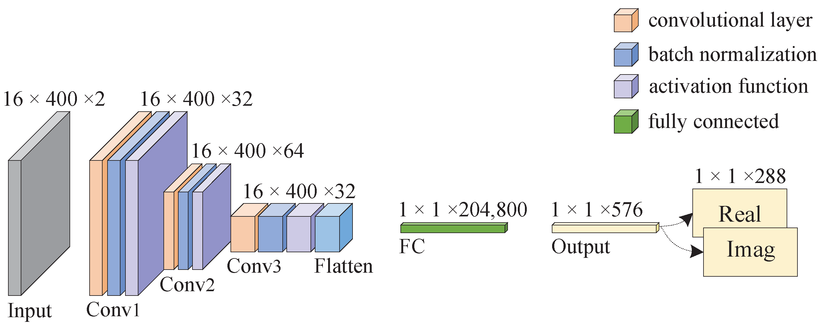
For adaptive time-domain beamforming technology, when the snapshots N is insufficient, it will result in severe distortion response to the wideband SOIs and poor suppression for interference. To obtain a satisfactory performance on wideband beamforming with certain DOAs of interference and insufficient snapshots, a method combining CNN structure with adaptive wideband FCFB, that is, WBPNet, is proposed in this paper. In general, the received signal $\mathbf{x}\left(n\right),n=1,2,\dots ,N$ is fed to the input layer of the network, and weights vector ${\mathbf{w}}_{CNN}$ are generated from the trained net as the predicted data. The final output successfully suppresses the interference in certain range even under the condition of extremely low snapshots, by utilizing the strong parallel processing ability and learning capacity that CNN equipped [30]. The specific design is introduced in the following subsections.

3.1. WBPNet Model

The WBPNet is designed on the basis of CNN, and the novel structure is shown in Figure 2. The WBPNet is mainly composed of three parts, namely, data samples, feature extraction and regression. Firstly, data samples are generated from the signal $\mathbf{x}\left(n\right)$ received at the array, and all training and testing samples are obtained under the circumstance of few snapshots. Then these data samples are divided into real and imaginary parts and transmitted to a dual-channel, because the input signal are complex-valued numbers containing both magnitude and phase information. Therefore, one simple approach to transfer the phase information, which is embedded in complex-valued received signal $\mathbf{x}\left(n\right)$, into the conventional real-valued CNNs is to employ two channels where magnitude and phase are taken as input [14]. It should be noted that the real and imaginary parts of data samples $\mathbf{x}\left(n\right)$ will be normalized before sent to the input layer of WBPNet and the specific normalization method will be introduced in Section 3.2. Then, CONV layers in the second phase would perform mapping between inputs and outputs, namely, feature extraction. In this stage, outputs employed for training process is the optimum weights obtained by using sufficient snapshots in (9). Therefore, the auto-correlative matrix inversion in analytic solution in conventional wideband time-domain beamforming algorithm is prevented by the nonlinear mapping processing in CNN, and the calculation speed of adaptive weight vectors based on the proposed WBPNet is faster. Then, these learned features are aggregated to execute fully connected (FC) operation after they are flatten. Finally, in the process of regression, the trained WBPNet can predict proximal optimal weights ${\mathbf{w}}_{opt}$ although the number of snapshots is very few. This property is reflected by giving the network a new set of data samples generated in few snapshots but acquire ideal weights. After regression, the obtained data in output layer are expanded as one-dimensional data, the output data are actually the weights ${\mathbf{w}}_{CNN}$. When these output data are used for simulation processing in MATLAB, they need to be reconstructed into the corresponding complex form. The scale of the WBPNet will be explained in the subsequent section. Since the proposed WBPNet uses few numbers of snapshots, the approaches require less processing time.

The detailed WBPNet approach is present in Figure 3. Generally, the CNN includes input layer, CONV layers, batch normalization (BN) layers, FC layers and output layers [31]. The following will introduce in detail the design of each layer of the proposed CNN-based WBPNet in this paper. The normalized training data samples are fed through a two-channel input layer before entering the CONV1 layer. The gradient vanishing problem can receive considerable alleviation from activation function ReLU, but the risk of dying neurons renders ReLU vulnerable. Thus many variants, such as LeakyReLU, are presented to fix this shortcoming [32]. In this paper, the activation function is LeakyReLU for all three CONV layers to solve the problem of gradient disappearance, and each layer also uses BN layer to accelerate the training [33]. Generally, neural networks have a large number of parameters. Therefore, overfitting is a serious problem in such networks. To address this problem, the approach of dropout, which is an avoiding overfitting technique, is applied to various models [34]. Thus, we apply a dropout in each layer to avoid overfitting. In the end of the third CONV layer, a flatten operation is constructed. The flatten operation reshapes the output acquired in three CONV layers of the WBPNet into one-dimensional data, and then transmitting them to the FC layer as the input during the regression phase. The specific parameters about the scale of each layer are demonstrated in Figure 3, they are relevant to the elements M, time-domain delay structures K and snapshots N mentioned in Section 2.

Therefore, different from most conventional CNNs, which are broadly used to realize image classification and image recognition, thereinto, CNNs based on classification will eventually output which kind of image is most likely in these categories. Therefore, the amount of data in the FC layer and the output layer in these research works is relatively small. We convert the problem into building CNN model of adaptive wideband beamforming, that is, the complex weights are divided into the real part and the imaginary part. In addition, all the real data in the two parts are the outputs, which is mapped by the network. Therefore, in Figure 3, the data scale of FC layer is sizable and equal to 204800. Moreover, the size of output layer corresponds to the optimal weights obtained through M arrays and K taps. For array models with different number of antennas or taps, our network parameters of output layer need to be redesigned. So, the size of the FC layer in Figure 3 corresponds to the case of 400 snapshots, which is a low number for the wideband beamforming. If the number of snapshots during the generation of training data increases, under the same design of output layer and CONV layers, the amount of data in the FC layer will be larger after the final flatten operation.

3.2. Training the WBPNet

The performance of adaptive wideband time-domain beamformers will be seriously damaged when snapshots N are few, and choosing covariance matrix as inputs will further increase computational complexity. Therefore, the proposed WBPNet selects $\mathbf{x}\left(n\right),n=1,2,\dots ,N$ as training inputs. Thereinto, $\mathbf{x}\left(n\right)$ is the signal vector that M antenna received in case of few snapshots. For convenience following, it is written as $\mathbf{x}$. In order to eliminate the influence of unit and scale differences between features, while treat each dimension features equally, features need to be normalized [35]. Therefore, training samples ${\mathbf{x}}_{train}$ are written as

$${\mathbf{x}}_{train}=\frac{\mathbf{x}-min\left(\mathbf{x}\right)}{max\left(\mathbf{x}\right)-min\left(\mathbf{x}\right)}$$

(10)

where, ${\mathbf{x}}_{train}$ are composed of the real and imaginary parts of $\mathbf{x}$. Since we adopt a double-channel input, the 1-st dimension and the 2-nd dimension of the double-channel correspond to the real and imaginary parts of ${\mathbf{x}}_{train}$, respectively. $\mathbf{x}\left(n\right)$ is divided into real and imaginary part firstly, and then normalized severally. Finally, the normalized real and imaginary parts are input through dual channels to form the ${\mathbf{x}}_{train}$ of the WBPNet.

Assuming the DOAs of interference are unknown but within a certain range, we perceive the direction of interference in certain angle area. Therefore, the proposed WBPNet conducts training on the certain range DOAs of interference, that is, ${\theta }_{j_i}\in [{\theta }_{j_{min}},{\theta }_{j_{max}}],i=1,2,\dots ,J$. Thereinto, J is the total number of DOAs of interference, and ${\theta }_{j_{min}}$ is the minimum DOA of interference, ${\theta }_{j_{max}}$ is the maximum DOA of interference. Therefore, the WBPNet has certain universal applicability when performing online. The information of these DOAs is contained in the normalized input vector ${\mathbf{x}}_{train}$. Similarly, the dimension of labels ${\mathbf{w}}_{opt}$ used in the WBPNet are required to be reshaped for matching the inputs with J interference angles. After the pre-process, the I/O pairs required in the WBPNet can be expressed as $({\mathbf{x}}_{train},{\mathbf{y}}_{train})$. (9) is used to obtain all the optimal weights corresponding to J DOAs of interference, which is the final ${\mathbf{y}}_{train}$. The procedure of training the WBPNet is shown in Algorithm 1.

Algorithm 1: WBPNet Training.

1: Input: ${\mathbf{x}}_{train}$, $\phi$, ${\mathbf{y}}_{train}$, $\eta$ and the number of epoch E

2: Initialization: ${\mathbf{W}}_i$, ${\mathbf{b}}_i\left(i=0,1,2,3\right)$ using the Kaiming criteria; $l\_\mathrm{best}=999$

3: for $e=0$: E, do

4: if ($e\%20==0$) do    $\eta \leftarrow \eta \phi$    else $\eta \leftarrow \eta$     ifend

5:  CONV1: ${\mathbf{x}}_{e1}\leftarrow \mathrm{dropout}\left(\mathrm{LeakyReLU}\left(\mathrm{BN}\left({\mathbf{x}}_{train}\ast {\mathbf{W}}_0+{\mathbf{b}}_0\right)\right)\right)$

6:  CONV2: ${\mathbf{x}}_{\mathrm{e}2}\leftarrow \mathrm{dropout}\left(\mathrm{LeakyReLU}\left(\mathrm{BN}\left({\mathbf{x}}_{\mathrm{e}1}\ast {\mathbf{W}}_1+{\mathbf{b}}_1\right)\right)\right)$

7:  CONV3: ${\mathbf{x}}_{e3}\leftarrow \mathrm{dropout}\left(\mathrm{LeakyReLU}\left(\mathrm{BN}\left({\mathbf{x}}_{e2}\ast {\mathbf{W}}_2+{\mathbf{b}}_2\right)\right)\right)$

8:  FC:$\mathbf{y}\leftarrow \mathrm{flatten}\left({\mathbf{x}}_{e3}\right){\mathbf{W}}_3+{\mathbf{b}}_3$

9: $l\leftarrow L\left({\mathbf{y}}_{train},\mathbf{y}\right)$, where l is the residual error, L is the loss function and we use MSE criterion.

10: if ($l<l\_\mathrm{best}$) do

$\stackrel{\wedge }{{\mathbf{W}}_i}\leftarrow {\mathbf{W}}_i$, $\stackrel{\wedge }{{\mathbf{b}}_i}\leftarrow {\mathbf{b}}_i$, $l\_\mathrm{best}\leftarrow l$

ifend

11:  back-propagation: $\left\{\begin{array}{c}{{\mathbf{W}}_i}^{\prime }\leftarrow {\mathbf{W}}_i-\eta \frac{\partial \mathrm{L}\left(\mathbf{W},\mathbf{b}\right)}{\partial {\mathbf{W}}_i}\hfill \\ {{\mathbf{b}}_i}^{\prime }\leftarrow {\mathbf{b}}_i-\eta \frac{\partial \mathrm{L}\left(\mathbf{W},\mathbf{b}\right)}{\partial {\mathbf{b}}_i}\end{array}\right.$

12: ${\mathbf{W}}_i\leftarrow {{\mathbf{W}}_i}^{\prime }$, ${\mathbf{b}}_i\leftarrow {{\mathbf{b}}_i}^{\prime }$

13: forend

14: output:${\mathbf{W}}_i\_\mathrm{best}\leftarrow \stackrel{\wedge }{{\mathbf{W}}_i}$, ${\mathbf{b}}_i\_\mathrm{best}\leftarrow \stackrel{\wedge }{{\mathbf{b}}_i}$

In Algorithm 1, I/O pairs $({\mathbf{x}}_{train},{\mathbf{y}}_{train})$, learning rate $\eta$ with its adjustment parameter $\phi$ and the number of epochs E are transmitted to the net. ∗ is the convolution operation. First of all, we use a step method to change the learning rate, that is, the learning rate $\eta$ will be adjusted adaptively every 20 epochs, which can make the training process more flexible [36]. In addition, the optimizer used to update weights in WBPNet is the Adam optimizer [37]. To be specific, we apply a step scheduler to adjust the learning rate shown as Step 4 in Algorithm 1. The detailed expression for each epoch can be given as (11)

$$\eta ={\eta }_0{\phi }^{floor\left(\frac{e}{20}\right)}$$

(11)

where the initial learning rate ${\eta }_0$ is $0.001$, $floor(•)$ function represents round a number down to the nearest integer. Some initial values such as ${\eta }_0$ and $\phi$ are empirically chosen [38] according to extensive numerical simulations, which has little impact on the algorithm performance since they will be learned and altered afterwards [39].

In each CONV layer, ${\mathbf{W}}_i$ represents the weight vector of the i-th layer convolutional kernel, and ${\mathbf{b}}_i$ is the i-th layer offset vector. Both of them are initialized under the criterion of Kaiming [40] to make the distribution of each layer as equal as possible. This method prevents the problem of gradient vanishing or gradient explosion and accelerate model convergence.

Before entering the FC layer, the WBPNet executes the flatten operation to reshape the output of the anterior CONV3 layer into a one-dimensional vector. Through aboving forward feedback, the output y is obtained in the FC layer and entered into the loss function. The training target is minimizing loss function $L({\mathbf{y}}_{train},y)$. Through constantly updating the $l\_\mathrm{best}$ during forward-propagation calculation, the network parameters $\mathbf{W}$ and $\mathbf{b}$ are renewed in back-propagation process.

In the proposed WBPNet, we employ the mean square error (MSE) function as the training loss function. The difference between the expected value and the actual value calculated by the MSE function after forward-propagation is called the residual errors [41]. The loss function is expressed as

$$L=\sum _{q=1}^Q\frac{{\left|y_{trai{n}_q}-y_q\right|}^2}{Q}$$

(12)

where Q is the final number of outputs.

During every epoch, when the current residual error l calculated from loss function, is smaller than $l\_\mathrm{best}$, the net renews the trainable variates $\stackrel{\wedge }{{\mathbf{W}}_i}$ and $\stackrel{\wedge }{{\mathbf{b}}_i}$, meanwhile $l\_\mathrm{best}$ is also updated by the current l. For future training, residual errors are propagated reversely through back-propagation, which is essentially a chain derivative plus gradient descent. Thus, parameters ${\mathbf{W}}_i$ and ${\mathbf{b}}_i$ of the CNN can be updated layer by layer through this method. The detailed gradient descent expression is shown as Step 12 of Algorithm 1, where learning rate $\eta$ can control the intensity of residual errors during back-propagation.

Once the trained net is accomplished with representative samples, the WBPNet will successfully build the mapping of anticipant $({\mathbf{x}}_{train},{\mathbf{y}}_{train})$ pairs. In the prediction phase, that is, online performance, the WBPNet is expected to respond to a set of verified inputs. It should be stressed that the WBPNet has never encountered these verified inputs. Besides, the samples for verification are generated in the case of few snapshots, indicating that these data have approximate distribution characteristics with the training data. From the results of the simulations, we successfully use CNN to realize the prediction network namely WBPNet. Instead of outputting the predicted categories in image classification techniques, the WBPNet finally outputs the weights using for adaptive wideband time-domain beamforming. The conventional FCFB algorithm obtains the optimal weights from (9), which involving calculation of covariance matrix and its inverse matrix. The WBPNet replaces this process through its own strong learning ability and fitting characteristics. Moreover, it takes a very small number of snapshots to reach ideal weights.

4. Simulation Results

In this section, certain simulation results are revealed to explain the validity and accuracy of the proposed WBPNet. Beampattern and array gain (AG) are two key metrics for beamformer performance evaluation [42]. Several abbreviations are used for the sake of distinction and convenience. In accordance with whether the snapshots are sufficient or not, the FCFB algorithm is classified as FCFB-few-snapshots (FCFB-FS) and FCFB-more-snapshots (FCFB-MS), and the proposed WBPNet is always operated under few-snapshots, namely, WBPNet-FS.

All simulation consequences are generated in the following situations: The number of TDLs K is 18, the array number M is 16; $f_{min}$ is 800 MHz and all frequency bands are 300 MHz. The number of more-snapshots $N_{more}$ is 4000. The frequency band is uniformly decomposed into $I=10$ bins. One wideband beam SOI comes from the direction ${\theta }_0$ of $5^{\circ }$, and interferences ${\theta }_j$ are in the range of $[-{60}^{\circ },-{30}^{\circ }]$ with $1^{\circ }$ interval, what means the number of wideband interference signal is totally 31. To avoid listing the entire 31 interferences one by one, we randomly select three groups of interference angles ${\theta }_{j_1}$, ${\theta }_{j_2}$, ${\theta }_{j_3}$: $-{60}^{\circ }$, $-{40}^{\circ }$, $-{30}^{\circ }$ to display. Furthermore, the signal to noise ratio (SNR) is 0 dB, and the interference to noise ratio (INR) is 40 dB. The Gaussian white additive noise is considered. In terms of arguments about the WBPNet, stride and padding are both 1 to keep the size of feature map; For each pair of wideband beam angle (${\theta }_0$, ${\theta }_j$), the number of training samples is 500, and that of testing samples is 10. The extent of dropout is $0.5$ in each layer. The size of convolution kernel $ke$ in each layer is 3. The number of input-channels is 2, 32 and 64, and the output-channels are 32, 64 and 32. Final output number in the FC layer is 576, that is, the number of approached elements mentioned in Section 3.1 is 576.

The simulation environment is based on Python $3.6.0$ with Pytorch $1.10.0$ on a host computer with I7-10700K CPU, and its main frequency is $3.8$ GHz. The video card is RTX 3060 with 12 GB video memory, 1780 MHz acceleration frequency and 3584 CUDA cores. The FCFB algorithm and the WBPNet are programmed on Python. The beampatterns are plotted in MATLAB after saving the output data from the WBPNet.

Figure 4 shows several beampatterns of the FCFB-FS, the FCFB-MS and the proposed WBPNet-FS in different DOAs of interference. The WBPNet-FS is designed based on the training sets generated by different few snapshots, respectively, and the weights obtained are displayed in the form of beampatterns. It should be emphasized here that, beampatterns of each WBPNet-FS are infinitely close to the corresponding beampatterns of FCFB-MS while they can also suppress total 31 DOAs of interference in the set $[-{60}^{\circ },-{30}^{\circ }]$ region. Each WBPNet trained under the condition of different few snapshots can achieve the beampatterns effect as shown in Figure 4. In addition, beampatterns for the FCFB-MS in $N_{more}$ are also included, whose weights are the labels when training. The accuracy of the DOA is $0.1^{\circ }$. In accordance with Figure 4a,d,g, the FCFB-FS algorithm apparently fails to gain undistorted response to the SOI neither generates nulls in interferences when N is far below normal. Those indicate that few snapshots result in scanty sampling numbers, thereby contributing to the failure in giving corresponding responses to the SOI and interferences. Conversely, the proposed WBPNet-FS has undistorted response to the SOI and forms deep nulls effective to anti-jamming, which vividly present in Figure 4b,e,h. Meanwhile, the Figure 4c,f,i are beampatterns of FCFB-MS, and they are also the ideal beampatterns, what the proposed WBPNet expected to achieve. The comparison of Figure 4b,e,f, with Figure 4c,f,i, proves that the WBPNet-FS achieves nearly identical beampatterns as the labels used in ${\mathbf{y}}_{train}$. Hence, Figure 4 distinctly verifies that the proposed WBPNet based on CNN has superior performance in case of particularly few snapshots, but the FCFB-FS algorithm is unable to realize. This advantage of the proposed WBPNet requires less processing time to achieve optimal weights.

The comparison results of Figure 4 can also be concluded as

Table 1. The performances of existing and proposed algorithms on beampatterns.

	FCFB-FS	FCFB-MS	WBPNet-FS (Proposed)
	($\mathit{N}=400$)	($\mathit{N}=4000$)	($\mathit{N}=400$)
Undistorted response to the SOI	x	√	√
Deep nulls to anti-jamming	x	√	√

. When $N=400$, the proposed WBPNet-FS performs well both on forming undistored response to the SOI and generating deep null for the interference. However, the traditional FCFB algorithm has a satisfactory performance on beampattern only with $N=4000$.

In order to study the influence of different low snapshots to the proposed network, the different few snapshots are used to generate corresponding training samples, which are used as the input of WBPNet. The few-snapshots $N_{few}$ used for comparing is 50, 100, 150, 200, 250, 300, 350, 400, respectively. With the same training conditions and network design, WBPNets of receiving signal in low snapshots are realized respectively.

Table 2. The output SINR (dB) under different snapshots N for comparison.

Direction	FCFB-FS	FCFB-MS		WBPNet-FS (Proposed)
	($\mathit{N}=400$)	($\mathit{N}=4000$)
			$\mathit{N}$	50	100	150	200	250	300	350	400
$({\theta }_0,{\theta }_{j_1})$	$-13.4808$	$4.5515$		$4.1722$	$4.3071$	$4.3240$	$4.3824$	$4.4421$	$4.4693$	$4.4859$	$4.4885$
$({\theta }_0,{\theta }_{j_2})$	$-12.5862$	$4.5512$		$4.1294$	$4.2584$	$4.2825$	$4.3358$	$4.3892$	$4.4076$	$4.4452$	$4.4571$
$({\theta }_0,{\theta }_{j_3})$	$-12.6891$	$4.5273$		$4.0932$	$4.2211$	$4.2567$	$4.2978$	$4.3573$	$4.3729$	$4.4085$	$4.4326$

demonstrates the output SINR of different snapshots conditions. Since the white Gaussian white additive noise in the received signal is generated randomly every time during simulation, the output SINR values in the Table 2 have been processed by 40 Monte Carlo analyses. When the number of snapshots is enough and equals to 4000, the output SINR of FCFB-MS is $4.5515$, $4.5512$, and $4.5273$ under three groups of DOAs respectively. The adaptive weights obtained with the FCFB-MS algorithm is also the label used when training the WBPNet-FS. From (9), the optimal weight of FCFB algorithm depends on estimating the covariance matrix $R_{xx}$ of received signal under N snapshots. When N is few (such as 400), the performance of FCFB algorithm will be damaged due to the estimation error of $R_{xx}$. Obviously, when the snapshots N is extremely fewer than what is normally needed, the output SINR of FCFB-FS is poor whatever the direction of interference. As shown in Table 2, the output SINR of FCFB-FS ($N=400$) is around $-13$ dB.

On the contrary, the output SINR of the proposed WBPNet-FS is favorable. When the number of snapshots is insufficient, the proposed WBPNet-FS carries out simulation research for different few snapshots $N_{few}$. As present in Table 2, with the increase of snapshots N, the output SINR of WBPNet-FS also gradually increases. Finally, when the number of snapshots is 400, the corresponding output SINRs of the three pairs of DOAs groups are respectively $4.4885$, $4.4571$ and $4.4326$. In the case of various low snapshots, the output SINR of FCFB-FS with $N=400$ is about 17 dB lower than that of WBPNet-FS with $N=50$. Thus, the output SINR of the proposed WBPNet-FS embodies its preponderance compared with the FCFB-FS. Meanwhile, the output SINR of FCFB-MS is used as reference, which is generated under $N_{more}$. Even when $N_{few}$ is several thousand less than $N_{more}$, the output SINR of the WBPNet-FS is only $0.01$ dB lower than that of FCFB-MS. The result also illustrates that the proposed WBPNet effectively reduces the waiting time of adaptive time-domain wideband beamformers.

Table 3. The multiplications of the WBPNet with analytical solution.

	FCFB-FS/FCFB-MS	WBPNet (Proposed)
Estimate the covariance matrix	$N\times {\left(MK\right)}^2$	Conv1	$M\times N\times k{e}^2\times C_{i_1}\times C_{o_1}$
The inversion of covariance matrix	$O\left[{\left(MK\right)}^3\right]$	Conv2	$M\times N\times k{e}^2\times C_{i_2}\times C_{o_2}$
Obtain the optimal weight vector	$O\left(I^3\right)+2I^{2}MK+I[2{MK}^2+MK]$	Conv3	$M\times N\times k{e}^2\times C_{i_3}\times C_{o_3}$

gives the computational complexity of different algorithms, where $C_i$ and $C_o$ represent the number of input-channels and output-channels, respectively and the detailed value is explained in the simulation conditions mentioned previously and presented in Figure 3. Therefore, $C_{i_1}=2$, $C_{o_1}=32$; $C_{i_2}=32$, $C_{o_2}=64$ and $C_{i_3}=64$, $C_{o_3}=32$. What needs illustration is that after three CONV layers, the final multiplications operation in the FC layer is related with the snapshots and equals to $M\times N\times C_{o_3}\times (MK\times 2)$. Therefore, the computational complexity of FC layer corresponding to different few snapshots is also different. In the aspects of FCFB-FS or FCFB-MS, the computation complexity is displayed by the complex multiplications (CMs) [43] involved. The computational complexities for estimating the covariance matrix, the inversion of the covariance matrix and the optimal weight vector are $N\times {\left(MK\right)}^2$, $O{\left(MK\right)}^3$ and $O\left(I^3\right)+2I^{2}MK+I[2{\left(MK\right)}^2+MK]$ CMs, respectively. Meanwhile, the computational complexities in every CONV layer are decided by $M\times N$, $k{e}^2$, $C_i$ and $C_o$, severally. Given that the proposed WBPNet cannot handle complex numbers directly [44], so all multiplicative and additive operations are involved as real numbers or known as floating point operations (FLOPs). The FLOPs in every layer are related to the channel parameters and feature map size. However, the multiplication operation of complex number is divided into real and imaginary parts, indicating that 1 CM in the FCFB algorithm is equivalent to 4 FLOPs [45] in the proposed WBPNet. In accordance with Table 3, calculating the inversion of the covariance matrix involves a third power $O{\left(MK\right)}^3$, and the order of magnitude in the multiplications of WBPNet is much smaller, that is, $k{e}^2\times {\left(MK\right)}^2$. Moreover, with the consideration that 1 CM is 4 FLOPs, the multiplications of WBPNet are much less than that of FCFB-FS or FCFB-MS obviously. Therefore, the proposed WBPNet exhibits low computational complexity compared with the FCFB algorithm.

As illustrated in Figure 4, Table 1, Table 2 and Table 3, such conclusions are summarized as follows: when facing the same signal produced in few snapshots $N_{few}$, the WBPNet-FS exhibits its dominance in acquiring undistorted response to SOI while availably restraining interferences in the form of deep nulls compared with the FCFB-FS algorithm. Meanwhile, the beampattern performance of WBPNet-FS is perfectly consistent with the FCFB-MS. Then, the output SINR of the proposed WBPNet-FS is greatly higher than FCFB-FS, and approximately $0.01$ dB lower than the output SINR obtained at $N_{more}=4000$. Moreover, for certain scenarios where the direction is known, DOAs of interference required in this situation is within a certain range, thus the proposed WBPNet can sense the direction of the DOAs of interference within the angle range required in the scene. The proposed WBPNet quickly makes a correct judgment on the DOA of interference with the reserved experience through pre-learning, especially when encountering unfamiliar wideband beams that are never appeared in advance. Although the received signal used in the verification is not encountered by the WBPNet during the training, the network can obtain the required weight through the mapping relationship after a lot of data learning [46]. Thus, the WBPNet has certain universality in the DOAs of interferences for systems in specific known direction scenarios. Furthermore, compared with the necessity of calculating the covariance matrix and its inversion in (9) in the FCFB algorithm, which involves large CMs. The WBPNet avoids this process, it just need the received data from array of antennas and converting the analytic solution problem to feature mapping between I/O pairs. Ultimately, the proposed WBPNet has a dominance in terms of the computation complexity.

5. Conclusions

In this paper, a network based on CNN structure, namely WBPNet, is proposed to realize adaptive time-domain wideband beamforming without delay structures under insufficient snapshots. The performance of FCFB is seriously damaged in the case of few snapshots for adaptive approaches, and this problem is solved by utilizing the unique nonlinear characteristic of CNN with its powerful parallel processing and learning ability. Furthermore, we train the WBPNet within common interferential angles. Therefore, the WBPNet can rapidly estimate the DOAs of interference, accurately restrain jamming adaptively in the certain range and has undistorted response to the SOI even under the condition of extremely few snapshots. Finally, uninvolved calculation of the autocorrelation matrix inversion makes contributions to the reduced computational complexity for the WBPNet structure, that is, the nonlinear mapping between I/O pairs replaces the analytic solution algorithm, and the training inputs used are the received signal rather than the covariance matrix. Then, the proposed WBPNet finally obtains the optimal weights required in the adaptive wideband time-domain beamforming technology. Compared with the conventional wideband beamforming technology, the proposed WBPNet does not require sufficient snapshots but obtains the favourable performance, with low computational complexity. The simulation results highlight the effectiveness and feasibility of the proposed method in achieving accurate response to the SOI, swiftly suppressing diverse interferences, attaining satisfactory output SINR and reducing computational complexity.

References

1. Bollian, T.; Osmanoglu, B.; Rincon, R.; Lee, S.K.; Fatoyinbo, T. Adaptive antenna pattern notching of interference in synthetic aperture radar data using digital beamforming. Remote Sens. 2019, 11, 1346. [Google Scholar] [CrossRef] [Green Version]
2. Chang, S.; Deng, Y.; Zhang, Y.; Wang, R.; Qiu, J.; Wang, W.; Zhao, Q.; Liu, D. An Advanced Echo Separation Scheme for Space-Time Waveform-Encoding SAR Based on Digital Beamforming and Blind Source Separation. Remote Sens. 2022, 14, 3585. [Google Scholar] [CrossRef]
3. Younis, M.; Fischer, C.; Wiesbeck, W. Digital beamforming in SAR systems. IEEE Trans. Geosci. Remote. Sens. 2003, 41, 1735–1739. [Google Scholar] [CrossRef]
4. Wiesbeck, W. SDRS: Software-defined radar sensors. In Proceedings of the IGARSS 2001. Scanning the Present and Resolving the Future, IEEE 2001 International Geoscience and Remote Sensing Symposium (Cat. No. 01CH37217), Sydney, Australia, 9–13 July 2001; Volume 7, pp. 3259–3261. [Google Scholar]
5. Wen, W.; Ning, L.; Jun, T.; Yingning, P. Broadband digital beamforming based on fractional delay in SAR systems. In Proceedings of the 2009 2nd Asian-Pacific Conference on Synthetic Aperture Radar, Xi’an, China, 26–30 October 2009; pp. 575–578. [Google Scholar]
6. Zhang, B.; Xu, G.; Zhou, R.; Zhang, H.; Hong, W. Multi-Channel Back-Projection Algorithm for MMWave Automotive MIMO SAR Imaging with Doppler-Division Multiplexing. IEEE J. Sel. Top. Signal Process. 2022. [Google Scholar] [CrossRef]
7. Xu, G.; Zhang, B.; Chen, J.; Wu, F.; Sheng, J.; Hong, W. Sparse Inverse Synthetic Aperture Radar Imaging Using Structured Low-Rank Method. IEEE Trans. Geosci. Remote Sens. 2022, 60, 1–12. [Google Scholar] [CrossRef]
8. Nordholm, S.E.; Dam, H.H.; Lai, C.C.; Lehmann, E.A. Broadband beamforming and optimization. In Academic Press Library in Signal Processing; Elsevier: Amsterdam, The Netherlands, 2014; Volume 3, pp. 553–598. [Google Scholar]
9. Frost, O.L. An algorithm for linearly constrained adaptive array processing. Proc. IEEE 1972, 60, 926–935. [Google Scholar] [CrossRef]
10. Zhang, S.; Gu, Q.; Wu, X.; Luo, J.; Sheng, W. Non-Uniform Decomposition Method Used for Obtaining the Frequency-Constrained Matrix of Broadband Laguerre Beamforming. IEEE Wirel. Commun. Lett. 2022, 11, 1359–1363. [Google Scholar] [CrossRef]
11. Ebrahimi, R.; Seydnejad, S.R. Elimination of pre-steering delays in space-time broadband beamforming using frequency domain constraints. IEEE Commun. Lett. 2013, 17, 769–772. [Google Scholar] [CrossRef]
12. Xu, G.; Zhang, B.; Chen, J.; Hong, W. Structured Low-rank and Sparse Method for ISAR Imaging with 2D Compressive Sampling. IEEE Trans. Geosci. Remote Sens. 2022, 60, 1–14. [Google Scholar] [CrossRef]
13. Baskin, C.; Zheltonozhkii, E.; Rozen, T.; Liss, N.; Chai, Y.; Schwartz, E.; Giryes, R.; Bronstein, A.M.; Mendelson, A. Nice: Noise injection and clamping estimation for neural network quantization. Mathematics 2021, 9, 2144. [Google Scholar] [CrossRef]
14. Oveis, A.H.; Giusti, E.; Ghio, S.; Martorella, M. A Survey on the Applications of Convolutional Neural Networks for Synthetic Aperture Radar: Recent Advances. IEEE Aerosp. Electron. Syst. Mag. 2021, 37, 18–42. [Google Scholar] [CrossRef]
15. Kuno, Y.M.; Masiero, B.; Madhu, N. A neural network approach to broadband beamforming. In Proceedings of the 23rd International Congress on Acoustics (ICA 2019), Aachen, Germany, 9–13 September 2019; pp. 6961–6968. [Google Scholar]
16. Albawi, S.; Mohammed, T.A.; Al-Zawi, S. Understanding of a convolutional neural network. In Proceedings of the 2017 International Conference on Engineering and Technology (ICET), Antalya, Turkey, 21–23 August 2017; pp. 1–6. [Google Scholar]
17. Kalchbrenner, N.; Grefenstette, E.; Blunsom, P. A convolutional neural network for modelling sentences. arXiv 2014, arXiv:1404.2188. [Google Scholar]
18. Jeon, M.; Jeong, Y.S. Compact and accurate scene text detector. Appl. Sci. 2020, 10, 2096. [Google Scholar] [CrossRef] [Green Version]
19. Vu, T.; Van Nguyen, C.; Pham, T.X.; Luu, T.M.; Yoo, C.D. Fast and efficient image quality enhancement via desubpixel convolutional neural networks. In Proceedings of the European Conference on Computer Vision (ECCV) Workshops, Munich, Germany, 8–14 September 2018. [Google Scholar]
20. Gu, Y.; Wu, J.; Fang, Y.; Zhang, L.; Zhang, Q. End-to-End Moving Target Indication for Airborne Radar Using Deep Learning. Remote Sens. 2022, 14, 5354. [Google Scholar] [CrossRef]
21. Sallam, T.; Attiya, A.M. Convolutional neural network for 2D adaptive beamforming of phased array antennas with robustness to array imperfections. Int. J. Microw. Wirel. Technol. 2021, 13, 1096–1102. [Google Scholar] [CrossRef]
22. Ramezanpour, P.; Mosavi, M.R. Two-stage beamforming for rejecting interferences using deep neural networks. IEEE Syst. J. 2020, 15, 4439–4447. [Google Scholar] [CrossRef]
23. Ramezanpour, P.; Rezaei, M.J.; Mosavi, M.R. Deep-learning-based beamforming for rejecting interferences. IET Signal Process. 2020, 14, 467–473. [Google Scholar] [CrossRef]
24. Li, Y.; Yang, X.; Liu, F. Fast and robust adaptive beamforming method based on complex-valued RBF neural network. J. Eng. 2019, 2019, 5917–5921. [Google Scholar] [CrossRef]
25. Lin, T.; Zhu, Y. Beamforming design for large-scale antenna arrays using deep learning. IEEE Wirel. Commun. Lett. 2019, 9, 103–107. [Google Scholar] [CrossRef] [Green Version]
26. Lovato, R.; Gong, X. Phased antenna array beamforming using convolutional neural networks. In Proceedings of the 2019 IEEE International Symposium on Antennas and Propagation and USNC-URSI Radio Science Meeting, Atlanta, Georgia, 7–12 July 2019; pp. 1247–1248. [Google Scholar]
27. Mizumachi, M. Neural Network-Based Broadband Beamformer with Less Distortion. In Proceedings of the 23rd International Congress on Acoustics (ICA 2019), Aachen, Germany, 9–13 September 2019; pp. 2760–2874. [Google Scholar]
28. Fernandes, J.d.C.V.; de Moura Junior, N.N.; de Seixas, J.M. Deep learning models for passive sonar signal classification of military data. Remote Sens. 2022, 14, 2648. [Google Scholar] [CrossRef]
29. Brown, A.D. Electronically Scanned Arrays MATLAB® Modeling and Simulation; CRC Press: Boca Raton, FL, USA, 2017. [Google Scholar]
30. Ali, R.; Chuah, J.H.; Talip, M.S.A.; Mokhtar, N.; Shoaib, M.A. Structural crack detection using deep convolutional neural networks. Autom. Constr. 2022, 133, 103989. [Google Scholar] [CrossRef]
31. Huang, H.; Peng, Y.; Yang, J.; Xia, W.; Gui, G. Fast beamforming design via deep learning. IEEE Trans. Veh. Technol. 2019, 69, 1065–1069. [Google Scholar] [CrossRef]
32. Duan, B.; Yang, Y.; Dai, X. Feature Activation through First Power Linear Unit with Sign. Electronics 2022, 11, 1980. [Google Scholar] [CrossRef]
33. Xia, W.; Zheng, G.; Wong, K.K.; Zhu, H. Model-driven beamforming neural networks. IEEE Wirel. Commun. 2020, 27, 68–75. [Google Scholar] [CrossRef] [Green Version]
34. Zhang, J.; Lu, C.; Wang, J.; Yue, X.G.; Lim, S.J.; Al-Makhadmeh, Z.; Tolba, A. Training convolutional neural networks with multi-size images and triplet loss for remote sensing scene classification. Sensors 2020, 20, 1188. [Google Scholar] [CrossRef] [PubMed] [Green Version]
35. Zhu, X.; Qi, F.; Feng, Y. Deep-learning-based multiple beamforming for 5g uav iot networks. IEEE Netw. 2020, 34, 32–38. [Google Scholar] [CrossRef]
36. Smith, L.N. A disciplined approach to neural network hyper-parameters: Part 1–learning rate, batch size, momentum, and weight decay. arXiv 2018, arXiv:1803.09820. [Google Scholar]
37. Zhang, H.; Yang, N.; Huangfu, W.; Long, K.; Leung, V.C. Power control based on deep reinforcement learning for spectrum sharing. IEEE Trans. Wirel. Commun. 2020, 19, 4209–4219. [Google Scholar] [CrossRef]
38. Wang, X.; Li, W.; Chen, V.C. Hand Gesture Recognition Using Radial and Transversal Dual Micro-Motion Features. IEEE Trans. Aerosp. Electron. Syst. 2022, 58, 5963–5973. [Google Scholar] [CrossRef]
39. Liu, S.; Huang, Y.; Wu, H.; Tan, C.; Jia, J. Efficient multitask structure-aware sparse Bayesian learning for frequency-difference electrical impedance tomography. IEEE Trans. Ind. Inform. 2020, 17, 463–472. [Google Scholar] [CrossRef] [Green Version]
40. He, K.; Zhang, X.; Ren, S.; Sun, J. Delving deep into rectifiers: Surpassing human-level performance on imagenet classification. In Proceedings of the IEEE International Conference on Computer Vision, Santiago, Chile, 11–18 December 2015; pp. 1026–1034. [Google Scholar]
41. Martin-Donas, J.M.; Gomez, A.M.; Gonzalez, J.A.; Peinado, A.M. A deep learning loss function based on the perceptual evaluation of the speech quality. IEEE Signal Process. Lett. 2018, 25, 1680–1684. [Google Scholar] [CrossRef]
42. Wang, X.; Zhai, W.; Greco, M.; Gini, F. Cognitive Sparse Beamformer Design in Dynamic Environment via Regularized Switching Network. IEEE Trans. Aerosp. Electron. Syst. 2022. [Google Scholar] [CrossRef]
43. Golub, G.H.; Van Loan, C.F. Matrix Computations; JHU Press: Baltmore, MD, USA, 2013. [Google Scholar]
44. Sallam, T.; Abdel-Rahman, A.B.; Alghoniemy, M.; Kawasaki, Z.; Ushio, T. A neural-network-based beamformer for phased array weather radar. IEEE Trans. Geosci. Remote. Sens. 2016, 54, 5095–5104. [Google Scholar] [CrossRef]
45. Rong, J.; Liu, F.; Miao, Y. High-Efficiency Optimization Algorithm of PMEPR for OFDM Integrated Radar and Communication Waveform Based on Conjugate Gradient. Remote Sens. 2022, 14, 1715. [Google Scholar] [CrossRef]
46. Miao, P.; Yin, W.; Peng, H.; Yao, Y. Study of the performance of deep learning-based channel equalization for indoor visible light communication systems. Photonics 2021, 8, 453. [Google Scholar] [CrossRef]
Figure 1. Adaptive time−domain beamforming structure without delay structures.
Remotesensing 15 00712 g001
Figure 2. The WBPNet structure.
Remotesensing 15 00712 g002
Figure 3. Details of the WBPNet with 400 snapshots.
Remotesensing 15 00712 g003
Figure 4. Beampatterns of randomly selected pairs angles with different snapshots.
Remotesensing 15 00712 g004